Image-Label Recovery on Fashion Data Using Image Similarity from Triple Siamese Network - MDPI
←
→
Page content transcription
If your browser does not render page correctly, please read the page content below
technologies
Article
Image-Label Recovery on Fashion Data Using Image Similarity
from Triple Siamese Network
Debapriya Banerjee * , Maria Kyrarini                       and Won Hwa Kim

                                           Department of Computer Science and Engineering, The University of Texas at Arlington (UTA),
                                           Arlington, TX 76019, USA; maria.kyrarini@uta.edu (M.K.); won.kim@uta.edu (W.H.K.)
                                           * Correspondence: debapriya.banerjee2@mavs.uta.edu

                                           Abstract: Weakly labeled data are inevitable in various research areas in artificial intelligence (AI)
                                           where one has a modicum of knowledge about the complete dataset. One of the reasons for weakly
                                           labeled data in AI is insufficient accurately labeled data. Strict privacy control or accidental loss may
                                           also cause missing-data problems. However, supervised machine learning (ML) requires accurately
                                           labeled data in order to successfully solve a problem. Data labeling is difficult and time-consuming as
                                           it requires manual work, perfect results, and sometimes human experts to be involved (e.g., medical
                                           labeled data). In contrast, unlabeled data are inexpensive and easily available. Due to there not
                                           being enough labeled training data, researchers sometimes only obtain one or few data points per
                                           category or label. Training a supervised ML model from the small set of labeled data is a challenging
                                           task. The objective of this research is to recover missing labels from the dataset using state-of-the-art
                                           ML techniques using a semisupervised ML approach. In this work, a novel convolutional neural
                                           network-based framework is trained with a few instances of a class to perform metric learning.
                                           The dataset is then converted into a graph signal, which is recovered using a recover algorithm
                                           (RA) in graph Fourier transform. The proposed approach was evaluated on a Fashion dataset for
                                 accuracy and precision and performed significantly better than graph neural networks and other

                                           state-of-the-art methods.
Citation: Banerjee, D.; Kyrarini M.;
Kim, W.H. Image-Label Recovery on          Keywords: semisupervised learning; metric learning; signal recovery
Fashion Data Using Image Similarity
from Triple Siamese Network.
Technologies 2021, 9, 10. https://
doi.org/10.3390/technologies9010010
                                           1. Introduction
Academic Editors: Abdellah Chehri               Supervised learning [1,2] is an approach in Machine Learning (ML) for classification [3]
and Pedro Antonio Gutiérrez                or regression tasks [4], where a set of labeled data is used to train a prediction model.
Received: 31 October 2020                  However, in practice, obtaining sufficient labeled data for training a model can be difficult.
Accepted: 15 January 2021                  There may be a strict privacy-control policy that restricts one from obtaining labeled data
Published: 21 January 2021                 or human error that can cause false or missing labels in the dataset. Additionally, there
                                           may not be enough of a budget to obtain all information labeled by human annotators,
Publisher’s Note: MDPI stays neu-          especially when expert knowledge is needed for the annotations. For example, during the
tral with regard to jurisdictional clai-   COVID-19 pandemic, online shopping drastically increased, and shop owners needed to
ms in published maps and institutio-       update their products. Manually finding the category of each product is time-consuming,
nal affiliations.                          therefore, it is important to develop a framework that can automatically categorize new
                                           data on the basis of a small amount of labeled data. In this scenario, an approach called
                                           Semisupervised Learning (SSL) can be useful to solve the problem of weakly labeled data.
Copyright: c 2021 by the authors.
                                           SSL algorithms are applied in such cases where a very limited amount of label data along
Licensee MDPI, Basel, Switzerland.
                                           with a large number of unlabeled data are used as input. SSL algorithms learn a better
This article is an open access article
                                           prediction rule than supervised ML would learn if trained only on a small amount of label
distributed under the terms and con-       data. Considering this approach in mind, we designed a semisupervised framework to
ditions of the Creative Commons At-        detect the labels or categories of unlabeled data. The concept behind our approach is that
tribution (CC BY) license (https://        similar data points lie very close to each other in vector space. In this regard, our objective
creativecommons.org/licenses/by/           was to learn a similarity measure to detect the distance of data points in vector space and
4.0/).                                     then detect the labels of unlabeled data through label propagation.

Technologies 2021, 9, 10. https://doi.org/10.3390/technologies9010010                                  https://www.mdpi.com/journal/technologies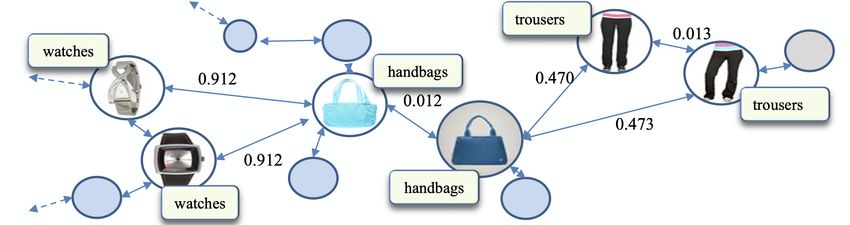
Technologies 2021, 9, 10                                                                                          2 of 16

                                Distance metric learning (DML) is a popular concept in modern ML research to learn
                           a similarity measure between two entities. DML aims at automatically constructing task-
                           specific distance metrics from data in an ML manner. It is often difficult to design metrics
                           that are well-suited to the particular data and task of interest. In this work, we designed a
                           novel DML model to detect the distance between every two images in an image dataset
                           with fashion products called the Fashion dataset [5], and then we propagated the label
                           information from a small subset of labeled data to the entire set of unlabeled data. It was
                           assumed that similar objects have a distance very close to zero and they share the same
                           label information. Figure 1 shows a visual representation of when similar objects share the
                           same label information.
                                The second component, label propagation, is a popular problem in SSL, where a small
                           subset of data points has label information, and the challenge is to propagate labels to the
                           unlabeled points from the labeled points through an algorithm. We adopted a method
                           introduced in [6] that exploits graph harmonics and sparse coding of graph signals in the
                           dual space of the graph. Here, we consider the labels of images as the graph signal on their
                           nodes, and the metric learned by DML consists of the edge between nodes (i.e., images).
                           In the end, our pipeline predicts the image labels of the entire dataset on the basis of a
                           small subset of images with given labels.

                           Figure 1. Visual representation of basic intuition.

                                In this work, we designed a novel approach combining DML and label propagation
                           for SSL. Our contributions are summarized as follows:
                           •    Designing a novel DML model to learn good similarity measures between every two
                                images in an image dataset and create a graph with their distances.
                           •    Recovering labels for all images from the graph using a label-propagation algorithm.
                                The rest of the paper is structured as follows: Section 2 describes related work,
                           Section 3 describes preliminary works that we performed as part of our experiments,
                           Sections 4 and 5 present our proposed methodology and implementation, and Section 6
                           discusses the numerical experiments.

                           2. Related Work
                                SSL [7] is an algorithm family that falls between supervised [1,2] and unsupervised
                           learning, making use of labeled and unlabeled data to perform learning tasks. For SSL, a
                           smaller set of labeled data in combination with a large set of unlabeled data are typically
                           used for the construction of a better learning technique. In recent years, due to the lack
                           of labeled data, SSL gained more popularity than supervised learning. Our model gained
                           inspiration from recent works on distance metric learning and label-propagation algorithms.
                           We provide a brief overview of the related work in both of these areas.
                                Label propagation is a way in which SSL detects the labels of unlabeled observa-
                           tions. Inductive learning [8] regards learning general rules for making predictions, while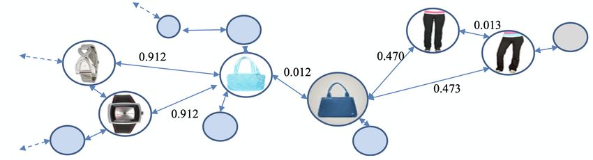
Technologies 2021, 9, 10                                                                                          3 of 16

                           transductive learning learns prediction rules from training data for specific testing data.
                           SSL is transductive, as labels are gradually predicted, and the model has to be retrained
                           whenever the testing set changes. In our case, labels were propagating, and if a new
                           instance (i.e., graph node) was added, the model had to be run again, so it was transduc-
                           tive. Puy et al. [9] first proposed the random sampling of band-limited signals on graphs.
                           Later, Kim et al. [10] proposed adaptive signal recovery on graphs via harmonic analysis
                           for experimental design in neuroimaging. Bronstein et al. [11] prepared an exhaustive
                           literature review paper, “geometric deep learning: going beyond Euclidean data”, on this
                           topic. Malkov et al. [12] first introduced the nearest-neighbor search using small world
                           problem. Saito et al. [13] proposed a semisupervised domain adaption technique via mini-
                           max entropy. Later, Zhai et al. [14] proposed a self-supervised SSL where they bridged the
                           gap between self-supervised and SSL.
                                 Work on one-shot and few-shot learning has gained popularity in DML. One-shot
                           learning is a learning task where there might be only one training example for a label or
                           category, and few-shot learning can be applied where there are only a few training examples
                           available for each label. One-shot learning is a way of learning similarity measures, and
                           it was first introduced by Bromley et al. [15] for signature verification using a Siamese
                           time-delay neural network. Then, Fei-Fei et al. [16] proposed a one-shot-based approach
                           for object categories. The authors assumed that currently learned classes can help to
                           make predictions on new ones when just one or few labels are available. Lake et al. [17]
                           presented a hierarchical Bayesian model that reached human-level error on few-shot
                           learning alphabet-recognition tasks. Koch et al. [18] presented a deep-learning model
                           based on computing the pairwise distance between samples using Siamese networks, and
                           Vinyals et al. [19] presented end-to-end trainable k-nearest neighbors using cosine distance.
                           Schroff et al. [20] proposed an anchor-based triple network for unified embedding called
                           FaceNet, which is useful for face recognition and clustering. The FaceNet model is trained
                           on the triplet loss function. Kertész et al. [21] proposed multidirectional image-projection
                           transformation with fixed vector lengths (MDIPFL) for one-shot learning, which performed
                           significantly better.
                                 Many recent works on SSL were based on generative models with deep neural net-
                           works. Few of such examples are graph neural networks (GNN) [22], variational autoen-
                           coders [23,24], and generative adversarial networks [25–27]. A GNN is a deep-learning
                           approach to deal with graph-structured data, and it was first proposed by Gori et al. [22].
                           Kim et al. [6] proposed a select-recovery-based model to recover multivariate signals in
                           an online manner using graph-signal processing. Kipf and Welling [28] proposed deep-
                           learning-based GNN models on semisupervised classification problems. Chang et al. [29]
                           develop graph interaction networks that learn pairwise particle interactions and apply
                           them to discrete particle-physical dynamics. Duvenaud et al. [30] and Kearnes et al. [31]
                           studied molecular fingerprints using variants of the GNN architecture, and Gilmer et al. [32]
                           further developed the model by combining it with set representations. Vinyals et al. [19]
                           showed state-of-the-art results on molecular prediction. Appalaraju et al. [33] proposed a
                           Siamese-network-based deep CNN model using curriculum learning and transfer learning
                           for image-similarity measurements.
                                 Our method is based on the combination of DML and a label-propagation algorithm.
                           We used a one-shot-learning [18,19] approach to learn DML and construct graphs on the
                           basis of distance learned from DML. Unlike traditional one-shot learning networks, we
                           propose a novel DML network that we combined with a label-propagation algorithm to
                           achieve the best results.

                           3. Preliminary Work
                                We focused on the Fashion dataset [5], which was downloaded from an online fashion
                           e-commerce store called Myntra. Although we focused on this dataset, this approach can be
                           applied to other image datasets or modalities. The fashion data consisted of a set of images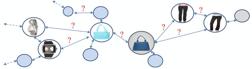
Technologies 2021, 9, 10                                                                                            4 of 16

                           of fashion products with their label information. Each of these images was processed to
                           grayscale and resized to 105 × 105 pixels. It was then processed to extract features.
                                 The one-shot-learning approach is a very popular technique to learn domain-specific
                           features from input images when the number of input images per class is limited. This
                           technique is very useful, even for DML, when the similarity measure is to be calculated
                           between input images. In this work, we used this approach as our baseline model to
                           calculate a good similarity measure between images. Koch et al. [18] focused on a twin
                           Siamese network to perform DML, and then reused that network’s features for one-shot
                           learning without any retraining.
                                 A twin Siamese network performs well for one-shot learning tasks, but training this
                           network is a time-consuming process. While training this network, it takes two inputs
                           at a time and calculates a similarity score from their distances. Therefore, the number of
                           comparisons was more (( Nk ) for N number of images and k is 2) to calculate the distance of
                           all images in our dataset. This twin Siamese network is sensitive with respect to context
                           and fails to capture fine-grain differences between two images. The above-mentioned
                           problems motivated us to focus on DML, creating a novel network that quickly converges
                           and captures fine-grained differences of labels.

                           4. Proposed Methodology
                                In this section, we discuss the design approach we propose. SSL is an approach
                           where a learning algorithm requires a small amount of training data and a large amount of
                           unlabeled data. Our goal in this research is to learn a prediction rule to detect the labels of
                           unlabeled datasets with the help of a small amount of labeled data points. We divided our
                           algorithm into two steps: distance metric learning and label propagation.

                           4.1. Distance Metric Learning
                                DML focuses on automatically constructing domain-specific distance metrics from
                           supervised data. In this step, our framework learns a good similarity measure between
                           two images. There are a few popular standard distance metrics, e.g., Euclidean distance
                           and cosine similarity, where we need prior knowledge of the domain. The aim of DML is
                           to construct a task-specific distance metric from a particular dataset.
                                Twin Siamese networks are one of the ways of learning distance between two images.
                           The concept of a twin Siamese network is that there are two parallel networks that share the
                           same weights. These two parallel networks are basically identical and learn the encoding
                           of input images. We used the twin Siamese network as our baseline model.
                                Our baseline model is a convolutional neural network (CNN) version of the twin
                           Siamese network, which takes two input images and learns the encoding of two input
                           images through this twin network. In the end, it learns the L1 distance of two feature vectors
                           and produces a distance score between 0 and 1 through a sigmoid layer. The detailed
                           architecture of this network is as follows: the model consists of a sequence of convolutional
                           layers, each of which uses a single channel with filters of varying size. The network applies
                           a rectified linear unit (ReLU) activation function to the output feature maps, followed by
                           max-pooling with a filter size and stride of 2.
                                Twin Siamese networks perform well compared to all other DML mentioned in
                           Section 2. However, Twin Siamese network performance is very slow. The convergence
                           time of this network is extremely large, taking almost 2000 epochs to converge. Detailed
                           hardware specifications are provided in Section 5.3. If we have an N number of images in
                           the dataset, the number of comparisons that happen in this network is ( Nk ), which is very
                           large to obtain the distance of every pair of images in our dataset. Therefore, we propose
                           the concept of a triple Siamese network to optimize these points.

                           4.1.1. Triple Siamese Network
                                In this network, we used three parallel networks that shared the same weights. The ar-
                           chitecture of each network is the same CNN network as the one that we used in the twin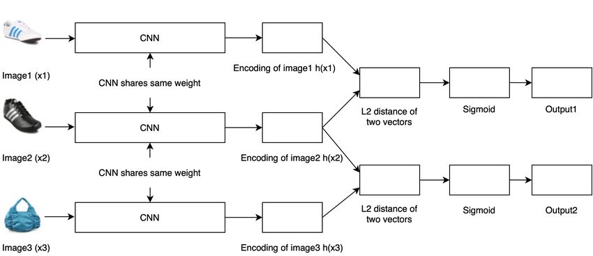
Technologies 2021, 9, 10                                                                                                     5 of 16

                           Siamese network. Through this network, we learned the similarity function as f ( x1 , x2 ),
                           where f ( x1 , x2 ) = ||h( x1 ) − h( x2 )||2 , here x1 and x2 are input images to the network, and
                           h( x1 ) and h( x2 ) are the encoding of x1 and x2 by the CNN. Figure 2 shows the system
                           architecture of the triple Siamese network.
                                 This network takes three images ( x1 , x2 , x3 ) as input in such a way that x2 and x1 are
                           taken from the same class, and x2 and x3 are taken from different classes. The goal is to
                           maximize the distance between x2 and x3 , and minimize the distance between x2 and x1 .
                           This network learns two L2 distances from these two pairs at a time.

                                            Figure 2. Triple Siamese network.

                           4.1.2. Graph Representation
                                After the triple Siamese Network provided the distance of each pair of images in
                           the Fashion dataset, we graphically represented our data. We have graph G = {V, E},
                           where V is a set of images, and E is the set of distances of each pair of images. Hence,
                           V = {v1 ,v2 . . . v N }, E = {eij , where eij = dist(vi ,v j )}, and N = total number of images. Figure 3
                           displays a graphical representation of the Fashion dataset [5].

                                  Figure 3. Graphical representation of image dataset.

                           4.2. Label Propagation
                                Label propagation determines the labels of unlabeled data from a very small amount
                           of labeled data. In this project, we considered the graph as graph signal and ran the RA
                           (Kim et al. [6]) on the graph. We recovered the graph signal using the harmonic analysis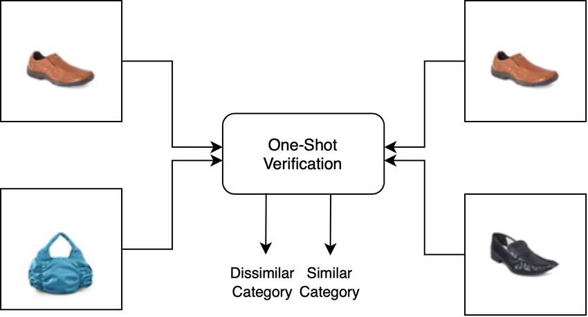
Technologies 2021, 9, 10                                                                                         6 of 16

                           of the graph. We applied two useful concepts, spectral graph theory [34] and harmonic
                           analysis of the graph [6,10], for our RA.

                           4.2.1. Spectral Graph Theory
                                Spectral graph theory [34] is the study of the properties of a graph in relationship to
                           the eigenvalues and eigenvectors of matrices associated with the graph, such as its distance
                           matrix or Laplacian matrix. Graph G = {V, E} is represented by a set of vertices V of
                           size N and a set of edges E that connect the vertices. Another matrix, graph Laplacian
                           L = D − W, where a degree matrix D N × N , is a diagonal matrix with the ith diagonal
                           element being the sum of edge weights connected to the ith vertex and WN × N being a
                           distance matrix where it is the most common way to represent a graph G, where each
                           element dij denotes the distance between the ith and jth vertices.

                           4.2.2. Graph Harmonic Analysis
                                Graph harmonic analysis [6,10] utilizes the Fourier/wavelet transform of the original
                           signal and filters in the frequency domain. The reason behind using harmonic analysis is
                           making use of sparsity in terms of representation obtained in the Fourier/wavelet space of
                           the graphs. By constructing different shapes of band-pass filters in the frequency space
                           and transforming them back into the original space, we can construct a mother wavelet ψ
                           on the nodes of a graph coming from its representation in the frequency space. For this
                           implementation, using spectral graph theory, we used orthonormal bases to design kernel
                           function g() in the space spanned by the bases. Graph Laplacian L provided eigenvalues
                           and corresponding eigenvector for N number of vertices. This eigenvector is used to define
                           the graph Fourier transform of a function f (n) defined on a vertex n. If signal f (n) lies
                           in the spectrum of the first k eigenvectors, then f (n) is k-band-limited. Graph Fourier
                           transform of a function f (n) is defined on vertices n as:

                                                                             N
                                                                 fˆ(l ) =   ∑       f (n)χ∗l (n)                    (1)
                                                                            n =1

                           and
                                                                              N
                                                                 f (n) =     ∑ fˆ(l )χl (n)                         (2)
                                                                             l =1

                           where χ is a set of eigenvectors that provide orthonormal bases, and χ∗ is a conjugate of χ.
                           Graph Fourier coefficient fˆ(l ) is obtained by forward transform, and the original function
                           f (n) can be reconstructed by the inverse transform.

                           4.2.3. Problem Setup
                                We formulated the problem setup as graph signal f ∈ R N × p , where measurement p
                           at each node is the one-shot encoding of the node labels, and N is a number of images or
                           nodes. We had an available partial observation at m vertices, where m
Technologies 2021, 9, 10 7 of 16
locations where we observed the signal can be denoted as ω = {ω1 , ω2 . . . ωm }. On the
basis of m observations, a projection matrix [6] Mm× N was built:
(
1, if j = ωi
Mij = (4)
0, o.w.
This framework solves Equation (3) entirely in a dual space by projecting the problem
to a low-dimensional space where we search for a solution of size kTechnologies 2021, 9, 10 8 of 16
L2 distance is passed through a sigmoid output to obtain the distance between two pairs
of inputs.
Figure 5 shows an example of a CNN architecture used in the triple Siamese network,
where three of these CNNs are used. Each CNN consists of a sequence of convolutional
layers with a single channel and filters of varying size, with a fixed stride of 1. This
architecture consists of a number of convolution layers as a multiple of 16. The ReLU
activation function is used on the output feature maps, followed by max- pooling with
a filter size and stride of 2. The 4096 unit fully connected layer was followed by another
layer where we calculated the L2 distance of each pair.
Figure 5. Architecture of a single convolutional neural network used in Siamese network.
5.1. Learning
We initialized all network weights in the convolutional layers from normal distribu-
tion with zero mean and a standard deviation of 10−2 . Biases were initialized from normal
distribution with mean 0.5 and standard deviation 10−2 . In the fully connected layers, bi-
ases were initialized in the same way as the convolutional layers were, but weights were
drawn from a much wider normal distribution with zero mean and standard deviation
2 × 10⁻² according to Koch et al. [18]. In the network, training is performed by feeding
the network with three samples (x1 , x2 , x3 ) at a time when x2 and x1 are of the same class,
and x3 is of a different class. The goal is to maximize the distance between x2 and x3 ,
and minimize the distance between x2 and x1 . At the top, there is a comparison layer
to compare both similarities, followed by a sigmoid layer to normalize the output in the
range of 0 and 1. We used mean square error (MSE) as the loss function. We tested our
model with triplet loss function and mean absolute error (MAE). The empirical results
showed that our model converged much faster in the case of the Fashion dataset with MSE
whereas MAE overfitted our model. Figure 6 shows the training and validation loss for
MAE. The back-propagation algorithm ran to simultaneously update the weights for all
three networks. Therefore, the loss function is:
Loss(s( f 1 ), s( f 2 )) = ||s( f 1 ), 1 − s( f 2 )||2 (9)
where s( f 1 ) is the sigmoid output of the first distance, and s( f 2 ) is the sigmoid output of
the second distance in Figure 2. Here, f 1 is the L2 -norm of the first two inputs (from the
same category), and f 2 is the L2 -norm of the second two inputs (from a different category).
Here, s( f 1 ) = 1 − s( f 2 ), as they are formed as a probability. Therefore, Equation (8)
can be rewritten as:
Loss(s( f 1 ), s( f 2 )) = α.(s( f 1 ))2 (10)
where α is a constant. Figure 7 shows that the triple Siamese network converged after
150 epochs while training on the Fashion dataset [5]. To obtain optimal results, the triplet
could be chosen through three strategies [21]: (i) random mining, (ii) semihard mining,
and (iii) hard mining. Our goal was to minimize the distance between positive pairs and
maximize the distance between negative pairs. As random mining is the most efficient
strategy [21], we used this mining technique for learning.Technologies 2021, 9, 10 9 of 16
MAE loss function training and validation loss
4.50
4.25
4.00
3.75
Loss
3.50
3.25
3.00
training
2.75 validation
0 20 40 60 80 100
Epoch
Figure 6. Mean absolute error (MAE) loss function for training and validation.
training accuracy
90
80
70
60
% Accuracy
50
40
30
20 Twin siamese network
Triple siamese network
0 20 40 60 80 100 120 140 160
Epoch
Figure 7. Average training accuracy calculated by performing 2-way one-shot learning.
5.2. Validation
For every pair of input images, this model generated a similarity score between 0 and 1.
N-way one-shot methods [18] were applied to measure the performance of this network.Technologies 2021, 9, 10 10 of 16
We considered N as 2 to perform one-shot learning, and repeated this k times to calculate
percentage of prediction p as:
(100 × n)
p= % (11)
k
where n is the number of correct predictions out of k trials. For validation, we used 50 trials.
Therefore, k was 50. Figure 8 shows the training and validation loss for MSE.
MSE loss function training and validation loss
4.5
4.0
Loss
3.5
3.0
2.5
training
validation
0 20 40 60 80 100
Epoch
Figure 8. Mean square error (MSE) loss function for training and validation.
5.3. Twin Siamese vs. Triple Siamese Network
The triple Siamese network converges very quickly compared to the twin Siamese
network. For example, the triple Siamese network converged in 7.5 min when training
on the Fashion dataset, while the twin Siamese network required 1.6 h. Training-system
characteristics: CPU 2.3 GHz, 8-Core Intel Core i9, memory 16 GB, 2667 MHz DDR4, GPU
AMD Radeon Pro 5500M 4 GB. To detect the distance between each pair of images in our
dataset, fewer comparisons were required in the triple Siamese network, and we obtained
two distance scores at a time. The triple Siamese network has two parallel layers to calculate
the distance metrics, which gives two distance measures at a time. This approach helps
to reduce training time in the triple Siamese network. The objective of using three layers
of a CNN network is to feed the network with three input images in such a way that two
images are from the same class, and the third is from a different class; then, we produce two
pairs (two from the same class and the other two from a different class) out of these three
input images to calculate two pairs of distance. This model helps to minimize the distance
between the two images in the first pair, and maximize the distance between the images in
the second pair. Through this model, we captured fine-grained differences between classes
that resided very closely in vector space.
6. Experiments and Results
In this section, we demonstrate the results of our algorithm using the Fashion dataset [5].
We downloaded the image dataset from the Myntra Fashion website, out of which we usedTechnologies 2021, 9, 10 11 of 16
1000 images for training, 1000 images for validation, and 4000 images for testing. Figure 9
shows the class distribution of the validation dataset.
70
60
50
number of images
40
30
20
10
0
Handbags
Bangle
Duffel_Bag
Backpacks
Capris
Caps
Churidar
Dupatta
Earrings
Belts
Bracelet
Compact
Flats
Kurtas
Leggings
Mufflers
Pendant
Shirts
Cufflinks
Clutches
Gloves
Heels
Jackets
Jeans
Shoes
Watches
Jumpsuit
Necklace
Camisoles
Dresses
Face_Moisturisers
Figure 9. Number of images per category in validation set.
The images had 31 different labels or categories, e.g., handbags, shirts, and shoes.
For our experiment, we first created a graph using our triple Siamese network with
the images, where images were defined as vertices or nodes, and edges denoted the
similarity score between two images. Measurements at each vertex were defined by
one-shot encoding of the label vector representing object labels where nonzero elements
indicated whether the corresponding objects existed in the image. As our dataset consisted
of 31 labels, each measurement was 1 × 31 vectors. Therefore, we obtained a f 4000×31
matrix for our entire image dataset, which served as the ground truth of our algorithm.
We assumed that our sample m was to be chosen using uniform random sampling and
mTechnologies 2021, 9, 10 12 of 16
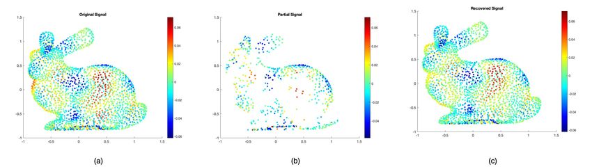
(a) Initial state.
(b) Metric learning.
(c) Label propagation.
Figure 10. Step-by-step operations of proposed method.
Results
After recovering the labels of all images in the Fashion dataset [5], we channeled our
output to a sigmoid layer to convert the recovered labels as binary. Since we chose our
sample by random uniform sampling, we performed each experiment 50 times to obtain the
average accuracy and average precision. We also computed the variance of accuracy and
precision of each model for different partial observations. We compared the performance
of our algorithm with that of random guess. Random guess [36] is the method of choosing
elements at random where they all have an equal chance of being chosen. Our algorithm
outperformed other baseline (random guess) and state-of-the-art algorithms, such as twin
Siamese, k-nearest neighbors (k-NN), and GNN. We show the performance of our triple
Siamese network with RA in Figure 11a,b.Technologies 2021, 9, 10 13 of 16
Accuracy Comparison Precision Comparison
Our Algorithm Our Algorithm
Twin Siamese network Twin Siamese network
kNN kNN
80 GNN 80 GNN
Random Guess Random Guess
60 60
% Accuracy
% Precision
40 40
20 20
0 0
200 400 600 800 1000 1200 1400 200 400 600 800 1000 1200 1400
Partial Observation Size Partial Observation Size
(a) Change in accuracy with respect to partial observations. (b) Change in precision with respect to partial observations.
Figure 11. Accuracy and precision comparison with respect to partial observations.
In Figure 11, we observed the performance of our algorithm with different samples
or partial-observation sizes. We sampled 5%, 10%, 18.75%, 25%, and 37.5% data points as
our partial observations, and recovered the signal using this. With a very small number
of samples (10% of sample size), our method performed significantly well compared to
other methods.
We compared the performance of our model with different partial-observation sizes,
and even with 400 partial-observation sizes out of 4000 data points, our model performed
significantly better than other models did. Tables 1 and 2 show the accuracy and precision
comparison of our model with respect to other models for different partial-observation
sizes, and the variance of the performance metrics with respect to partial observations.
Table 1. Accuracy comparison of our model with other models for different partial-observation (PO) sizes. Note: RA,
recover algorithm; k-NN, k-nearest neighbors.
P.O. 400 P.O. 750 P.O. 1000 P.O. 1500
Models
Acc Var Acc Var Acc Var Acc Var
Triple Siamese net and RA (our method) 60.91% 29.37 81.1% 22.45 83.7% 31.83 86.4% 27.32
Twin Siamese net and RA [18] 55.23 21.45 62.8% 12.87 70.2% 22.75 79.3% 17.20
Triple Siamese net and k-NN [37] 20.1 13.8 41.6% 26.92 50% 23.66 45.5% 9.25
Graph convolutional network [24] 12.81 15.2 17% 10.01 21.8% 17.21 23.7% 22.90
Table 2. Precision Comparison of our model with other models for different partial-observation sizes.
P.O. 400 P.O. 750 P.O. 1000 P.O. 1500
Models
Acc Var Acc Var Acc Var Acc Var
Triple Siamese net and RA(Our method) 57.32% 15.4 84.6% 18.67 85.5% 10.49 87.6% 9.41
Twin Siamese net and RA [18] 52% 17.77 71.4% 16.33 82.7% 17.71 82.8% 12.58
Triple Siamese net and k-NN [37] 39.71% 17.32 60.4% 32.79 65.8% 23.36 67.3% 18.63
Graph convolutional network [24] 13.32% 16.51 13.3% 15.62 17.4% 17.49 18% 17.22Technologies 2021, 9, 10 14 of 16
7. Conclusions
In this work, we introduce a novel approach for SSL in the Fashion dataset, where we
had a limited amount of labeled data to train our model. As the backbone of our algorithm,
we assumed that similar data points resided close to each other in vector space, and different
data points reside far away from each other in vector space. We then discussed a novel
algorithm for DML approaches to retrieve similarity measures from image-feature vectors.
Our DML model quickly converged and was able to capture fine-grain differences between
class labels. We also discussed the concept of spectral graph theory and the application of
harmonic analysis on the graph signal to recover the signal from our partially observed
graph data. Our algorithm performed significantly better than GCN and the twin Siamese
network did, even for the very small amount of labeled data in the Fashion dataset.
We plan to extend our work towards designing a generalized triple Siamese network in
combination with transfer learning [38], and evaluating its performance on other standard
image datasets in the same or different domains, such as the Fashion-MNIST dataset [39]
and ImageNet [40].
In the future, this work can be extended using different DML architectures such as
FaceNet [20]. This architecture is mainly used for classifying facial image datasets. The loss
function used in this model was triplet loss function, which can be further extended in our
framework.
Furthermore, this work can be extended towards other modalities using multimodal
fusion architectures [41], and can be compared with our framework for measuring perfor-
mance. Moreover, we aim to extend this work using active learning [42] and to evaluate
the performance of the framework.
Author Contributions: Conceptualization, D.B. and W.H.K.; methodology, formal analysis, design,
validation, D.B.; writing—original-draft preparation, D.B.; writing—review and editing, D.B., M.K.
and W.H.K.; supervision, project administration, and funding acquisition, W.H.K. All authors have
read and agreed to the published version of the manuscript.
Funding: This research was supported by NSF IIS CRII 1948510, NIH R01 AG059312, and IITP-2020-
2015-0-00742.
Institutional Review Board Statement: Not applicable.
Informed Consent Statement: Not applicable.
Conflicts of Interest: The authors declare no conflict of interest.
Abbreviations
The following abbreviations are used in this manuscript:
AI Artificial intelligence
ML Machine learning
DML Distance metric learning
CNN Convolutional neural network
MSE Mean square error
SSL Semisupervised learning
ReLU Rectified linear unit
GNN Graph neural network
k-NN k-nearest neighbors
MAE Mean absolute error
RA Recover algorithmTechnologies 2021, 9, 10 15 of 16
References
1. Niculescu-Mizil, A.; Caruana, R. Predicting good probabilities with supervised learning. In Proceedings of the ICML ’05, Bonn,
Germany, 7–11 August 2005.
2. Kotsiantis, S.B. Supervised Machine Learning: A Review of Classification Techniques. In Proceedings of the 2007 Conference on
Emerging Artificial Intelligence Applications in Computer Engineering: Real Word AI Systems with Applications in EHealth,
HCI, Information Retrieval and Pervasive Technologies, Amsterdam, The Netherlands, 14–16 June 2007; pp. 3–24.
3. Loog, M. Supervised Classification: Quite a Brief Overview. arXiv 2017, arXiv:cs.LG/1710.09230.
4. Stephen, P.; Jaganathan, S. Linear regression for pattern recognition. In Proceedings of the 2014 International Conference on Green
Computing Communication and Electrical Engineering (ICGCCEE), Coimbatore, India, 6–8 March 2014; pp. 1–6. [CrossRef]
5. Param, A. Fashion Product Images (Small). 2019. Available online: https://www.kaggle.com/paramaggarwal/fashion-product-
images-small (accessed on 20 January 2021).
6. Kim, W.H.; Jalal, M.; Hwang, S.; Johnson, S.C.; Singh, V. Online Graph Completion: Multivariate Signal Recovery in Computer
Vision. In Proceedings of the IEEE Conference on Computer Vision and Pattern Recognition (CVPR), Honolulu, HI, USA, 21–26
July 2017.
7. van Engelen, J.E.; Hoos, H. A survey on semi-supervised learning. Mach. Learn. 2019, 109, 373–440. [CrossRef]
8. Iscen, A.; Tolias, G.; Avrithis, Y.; Chum, O. Label Propagation for Deep Semi-supervised Learning. In Proceedings of the IEEE/CVF
Conference on Computer Vision and Pattern Recognition (CVPR), Long Beach, CA, USA, 16–20 June 2019; pp. 5070–5079.
9. Puy, G.; Tremblay, N.; Gribonval, R.; Vandergheynst, P. Random sampling of bandlimited signals on graphs. In Proceedings of
the NIPS2015 Workshop on Multiresolution Methods for Large Scale Learning, Montréal, QC, Canada, 12 December 2015.
10. Kim, W.H.; Hwang, S.J.; Adluru, N.; Johnson, S.C.; Singh, V. Adaptive Signal Recovery on Graphs via Harmonic Analysis
for Experimental Design in Neuroimaging. In Proceedings of the Computer Vision—ECCV 2016—14th European Conference,
Amsterdam, The Netherlands, 11–14 October 2016; Part VI; Lecture Notes in Computer Science; Leibe, B., Matas, J., Sebe, N.,
Welling, M., Eds.; Springer: Berlin/Heidelberg, Germany, 2016; Volume 9910, pp. 188–205. [CrossRef]
11. Bronstein, M.M.; Bruna, J.; LeCun, Y.; Szlam, A.; Vandergheynst, P. Geometric Deep Learning: Going beyond Euclidean data.
IEEE Signal Process. Mag. 2017, 34, 18–42. [CrossRef]
12. Malkov, Y.A.; Yashunin, D.A. Efficient and robust approximate nearest neighbor search using Hierarchical Navigable Small
World graphs. IEEE Trans. Pattern Anal. Mach. Intell. 2020, 42, 824–836. [CrossRef] [PubMed]
13. Saito, K.; Kim, D.; Sclaroff, S.; Darrell, T.; Saenko, K. Semi-supervised Domain Adaptation via Minimax Entropy. In Proceedings of
the IEEE/CVF International Conference on Computer Vision (ICCV), Seoul, Korea, 27 October–2 November 2019; pp. 8050–8058.
14. Zhai, X.; Oliver, A.; Kolesnikov, A.; Beyer, L. S4L: Self-Supervised Semi-Supervised Learning. In Proceedings of the IEEE/CVF
International Conference on Computer Vision (ICCV), Seoul, Korea, 27 October–2 November 2019; pp. 1476–1485.
15. Bromley, J.; Guyon, I.; LeCun, Y.; Säckinger, E.; Shah, R. Signature Verification using a “Siamese” Time Delay Neural Network.
In Advances in Neural Information Processing Systems; Cowan, J., Tesauro, G., Alspector, J., Eds.; Morgan-Kaufmann: Burlington,
MA, USA, 1994; Volume 6, pp. 737–744.
16. Fei-Fei, L.; Fergus, R.; Perona, P. One-shot learning of object categories. IEEE Trans. Pattern Anal. Mach. Intell. 2006, 28, 594–611.
[CrossRef]
17. Lake, B.M.; Salakhutdinov, R.; Tenenbaum, J.B. Human-level concept learning through probabilistic program induction. Science
2015, 350, 1332–1338. [CrossRef]
18. Koch, G.; Zemel, R.; Salakhutdinov, R. Siamese Neural Networks for One-shot Image Recognition. In Proceedings of the ICML
Deep Learning Workshop, Lille Grand Palais, France, 6–11 July 2015.
19. Vinyals, O.; Blundell, C.; Lillicrap, T.; Kavukcuoglu, K.; Wierstra, D. Matching Networks for One Shot Learning. Adv. Neural Inf.
Process. Syst. 2016, 29, 3630–3638.
20. Schroff, F.; Kalenichenko, D.; Philbin, J. FaceNet: A unified embedding for face recognition and clustering. In Proceedings of the
2015 IEEE Conference on Computer Vision and Pattern Recognition (CVPR), Boston, MA, USA, 8–10 June 2015. [CrossRef]
21. Kertész, G. Metric Embedding Learning on Multi-Directional Projections. Algorithms 2020, 13, 133. [CrossRef]
22. Gori, M.; Monfardini, G.; Scarselli, F. A new model for learning in graph domains. In Proceedings of the 2005 IEEE International
Joint Conference on Neural Networks, Montreal, QC, Canada, 31 July–4 August 2005; Volume 2, pp. 729–734.
23. Doersch, C. Tutorial on Variational Autoencoders. arXiv 2016, arXiv:stat.ML/1606.05908.
24. Kipf, T.N.; Welling, M. Variational Graph Auto-Encoders. arXiv 2016, arXiv:stat.ML/1611.07308.
25. Goodfellow, I.J.; Pouget-Abadie, J.; Mirza, M.; Xu, B.; Warde-Farley, D.; Ozair, S.; Courville, A.; Bengio, Y. Generative Adversarial
Networks. arXiv 2014, arXiv:stat.ML/1406.2661.
26. Odena, A. Semi-Supervised Learning with Generative Adversarial Networks. arXiv 2016, arXiv:stat.ML/1606.01583.
27. Salimans, T.; Goodfellow, I.; Zaremba, W.; Cheung, V.; Radford, A.; Chen, X. Improved Techniques for Training GANs. arXiv
2016, arXiv:cs.LG/1606.03498.
28. Kipf, T.N.; Welling, M. Semi-Supervised Classification with Graph Convolutional Networks. arXiv 2016, arXiv:1609.02907.
29. Chang, M.B.; Ullman, T.; Torralba, A.; Tenenbaum, J.B. A Compositional Object-Based Approach to Learning Physical Dynamics.
arXiv 2016, arXiv:1612.00341.
30. Duvenaud, D.; Maclaurin, D.; Aguilera-Iparraguirre, J.; Gómez-Bombarelli, R.; Hirzel, T.; Aspuru-Guzik, A.; Adams, R.P.
Convolutional Networks on Graphs for Learning Molecular Fingerprints. Adv. Neural Inf. Process. Syst. 2015, 28, 2224–2232.Technologies 2021, 9, 10 16 of 16
31. Kearnes, S.M.; McCloskey, K.; Berndl, M.; Pande, V.S.; Riley, P. Molecular graph convolutions: Moving beyond fingerprints.
J. Comput. Aided Mol. Des. 2016, 30, 595–608. [CrossRef]
32. Gilmer, J.; Schoenholz, S.S.; Riley, P.F.; Vinyals, O.; Dahl, G.E. Neural message passing for quantum chemistry. In Proceedings of
the 34th International Conference on Machine Learning, Sydney, Australia, 6–11 August 2017; Volume 70, pp. 1263–1272.
33. Appalaraju, S.; Chaoji, V. Image similarity using Deep CNN and Curriculum Learning. arXiv 2017, arXiv:1709.08761.
34. Hammond, D.K.; Vandergheynst, P.; Gribonval, R. Wavelets on Graphs via Spectral Graph Theory. App. Comput. Harmonic Anal.
2011, 30, 129–150. [CrossRef]
35. Turk, G.; Levoy, M. Zippered Polygon Meshes from Range Images. In Proceedings of the 21st Annual Conference on Computer
Graphics and Interactive Techniques (SIGGRAPH ’94), Orlando, FL, USA, 24–29 July 1994; pp. 311–318. [CrossRef]
36. Frary, R.B.; Cross, L.H.; Lowry, S.R. Random guessing, correction for guessing, and reliability of multiple-choice test scores.
J. Exp. Educ. 1977, 46, 11–15. [CrossRef]
37. Hui, G.G.; Wang, H.; Bell, D.; Bi, Y.; Greer, K. KNN Model-Based Approach in Classification. In Proceedings of the OTM
Confederated International Conferences On the Move to Meaningful Internet Systems, Catania, Italy, 3–7 November 2003.
38. Tan, C.; Sun, F.; Kong, T.; Zhang, W.; Yang, C.; Liu, C. A Survey on Deep Transfer Learning. In Proceedings of the International
Conference on Artificial Neural Networks, Rhodes, Greece, 4–7 October 2018.
39. Xiao, H.; Rasul, K.; Vollgraf, R. Fashion-MNIST: A Novel Image Dataset for Benchmarking Machine Learning Algorithms. arXiv
2017, arXiv:1708.07747.
40. Deng, J.; Dong, W.; Socher, R.; Li, L.J.; Li, K.; Fei-Fei, L. ImageNet: A Large-Scale Hierarchical Image Database. In Proceedings of
the 2009 IEEE Conference on Computer Vision and Pattern Recognition (CVPR09), Miami, FL, USA, 20–25 June 2009.
41. Vielzeuf, V.; Lechervy, A.; Pateux, S.; Jurie, F. CentralNet: A Multilayer Approach for Multimodal Fusion. In Proceedings of the
European Conference on Computer Vision (ECCV), Munich, Germany, 8–14 September 2018.
42. Settles, B. Active Learning Literature Survey (Computer Sciences Technical Report 1648); University of Wisconsin-Madison: Madison,
WI, USA, 2009.You can also read