A Comparative Study of Random Forest and Genetic Engineering Programming for the Prediction of Compressive Strength of High Strength Concrete ...
←
→
Page content transcription
If your browser does not render page correctly, please read the page content below
applied
           sciences
Article
A Comparative Study of Random Forest and Genetic
Engineering Programming for the Prediction of
Compressive Strength of High Strength Concrete
(HSC)
Furqan Farooq 1, *, Muhammad Nasir Amin 2 , Kaffayatullah Khan 2 ,
Muhammad Rehan Sadiq 3 , Muhammad Faisal Javed 1, * , Fahid Aslam 4                  and
Rayed Alyousef 4
 1    Department of Civil Engineering, COMSATS University Islamabad, Abbottabad Campus 22060, Pakistan
 2    Department of Civil and Environmental Engineering, College of Engineering, King Faisal University (KFU),
      P.O. Box 380, Al-Hofuf, Al Ahsa 31982, Saudi Arabia; mgadir@kfu.edu.sa (M.N.A.); kkhan@kfu.edu.sa (K.K.)
 3    Department of Transportation Engineering, Military College of Engineering (MCE), National University of
      Science and Technology (NUST), Risalpur 23200, Pakistan; rehansadiq04@gmail.com
 4    Department of Civil Engineering, College of Engineering in Al-Kharj, Prince Sattam bin Abdulaziz
      University, Al-Kharj 11942, Saudi Arabia; f.aslam@psau.edu.sa (F.A.); r.alyousef@psau.edu.sa (R.A.)
 *    Correspondence: furqan@cuiatd.edu.pk (F.F.); arbabfaisal@cuiatd.edu.pk (M.F.J.)

 Received: 23 August 2020; Accepted: 6 October 2020; Published: 20 October 2020

 Abstract: Supervised machine learning and its algorithm is an emerging trend for the prediction
 of mechanical properties of concrete. This study uses an ensemble random forest (RF) and gene
 expression programming (GEP) algorithm for the compressive strength prediction of high strength
 concrete. The parameters include cement content, coarse aggregate to fine aggregate ratio, water,
 and superplasticizer. Moreover, statistical analyses like MAE, RSE, and RRMSE are used to evaluate
 the performance of models. The RF ensemble model outbursts in performance as it uses a weak base
 learner decision tree and gives an adamant determination of coefficient R2 = 0.96 with fewer errors.
 The GEP algorithm depicts a good response in between actual values and prediction values with an
 empirical relation. An external statistical check is also applied on RF and GEP models to validate
 the variables with data points. Artificial neural networks (ANNs) and decision tree (DT) are also
 used on a given data sample and comparison is made with the aforementioned models. Permutation
 features using python are done on the variables to give an influential parameter. The machine learning
 algorithm reveals a strong correlation between targets and predicts with less statistical measures
 showing the accuracy of the entire model.

 Keywords: strength concrete; prediction; genetic engineering programming

1. Introduction
      High strength concrete (HSC) has its popularity spread wide and far for its superior performance.
HSC has been deemed superior for its substantial high strength and durability [1–4]. Its strength has
been witnessed to be higher than that of conventional concrete, a quality that has drastically increased
its use in the modern-day construction industry [5]. A new technology that results in homogenous and
dense concrete, and also bolsters the strength parameters, is the reason for the permeation in its use
within the construction industry [5,6]. It has been commonly used in concrete-filled steel tubes, bridges,
and columns. As per the American Concrete Institute (ACI), “HSC is the one that possesses a specific
requirement for its working which cannot be achieved by conventional concrete” [7]. Numerous

Appl. Sci. 2020, 10, 7330; doi:10.3390/app10207330                                www.mdpi.com/journal/applsci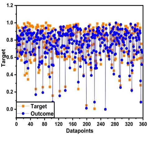
Appl. Sci. 2020, 10, 7330                                                                                  2 of 18

researchers suggested different methods for the mix design of HSC. All the methods of mix design
require a specific set of experimental trials to achieve the target strength. It is an ineluctable truth that
the experimental work is time consuming and requires a substantial amount of money. In addition,
amateur technicians and error in testing machines raise questions on the veracity of the experimental
work conducted across the globe. Various researchers used different statistical methods to predict
different properties of HSC. Some of the studies are summarized in Table 1. However, this field still
requires further exploration.

                      Table 1. Algorithm used in prediction properties of high strength concrete.

                       Properties                  Data Points           Algorithm            References
         Compressive strength, Slump test              187                ANN                        [7]
                Elastic modulus                        159                ANN                        [8]
                Elastic modulus                        159               FUZZY                       [9]
                Elastic modulus                        159                 SVM                      [10]
                Elastic modulus                        159          ANFIS and nonlinear             [11]
             Compressive strength                       20                ANN                       [12]
             Compressive strength                      324                 ELM                      [13]
             Compressive strength                      357                 GEP                      [14]

     In recent years, concepts of machine learning are used successfully in various fields for
the predictions of different properties. Likewise, the civil engineering construction industry has
also adopted such techniques to overcome cumbersome experimental procedures. For instance,
some of these approaches include multivariate adaptive regression spline (MARS) [15,16], genetic
engineering programming (GEP) [17–20], support vector machine (SVM) [21,22], artificial neural
networks (ANN) [23–25], decision tree (DT) [26–28], adaptive boost algorithm (ABA), and adaptive
neuro-fuzzy interference (ANFIS) [29–32]. Javed et al. [18] predict the axial behavior of a concrete-filled
steel tube (CFST) with 227 data points by using gene expression programming. The author achieves
adamant strong correlation between prediction and experimental axial capacity [18]. Farjad el al. [33]
used gene expression programming in the prediction of mechanical properties of waste foundry sand
in concrete. Gregor et al. [34] adopted the ANN approach to evaluate the compressive strength of
concrete. It was witnessed that ANN depicts the experimental values accurately; thus, it proves to
be an exceptional prediction tool. Amir et al. [35] predict the compressive strength of geopolymer
concrete incorporating natural zeolite and silica fume by using ANN. ANN thus established a good
relationship and gave obstinate accuracy in prediction of geopolymer concrete. Zahra et al. [32]
predict the compressive strength of concrete with ANN and ANFIS models. The authors reveal
that ANFIS gives a more adamant and stronger correlation than the ANN model. Javed et al. [36]
predict the compressive strength of sugar cane bagasse ash concrete by conducting the experimental
and literature-based study. Experimental work is used to validate the model and remaining data
were gathered from published literature. The author used the GEP algorithm and obtained a good
model between target values. Nour et al. [37] used the GEP algorithm to predict the compressive
strength of concrete filled steel columns incorporating recycled aggregate (RACFSTC). The author
used 97 data points in the modeling aspect of the RACFSTC column and observed adamant correlation.
Junfei et al. [38] modeled the compressive strength self-compacting concrete by using beetle antennae
search-based random forest algorithm. The author obtained an obstinate strong correlation of R2
= 0.97 with experimental results. Qinghua et al. [26] employed random forest approach to predict
the compressive strength of high-performance concrete. Similarly, Sun et al. [39] used evolved random
forest algorithm on 138 data samples to predict the compressive strength of rubberized concrete which
was collected from published literature. This advanced-based approach gave better performance
with a strong coefficient correlation of R2 = 0.96. ANN and other models have been adopted for
predicting the mechanical strength parameters of high-performance concrete and recycled aggregate
concrete [40–44]. Pala et al. [45] studied the influence of silica and fly ash on the compressive strength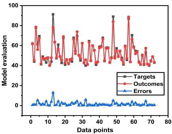
Appl. Sci. 2020, 10, 7330                                                                           3 of 18

of concrete. A comprehensive experimental was carried out to analyze the impact of varying w/c
ratios and varying percentages of silica and fly ash on the performance of concrete. In addition, ANN
was adopted to depict the effect on the strength parameters of concrete [45]. Azim et al. [44] used
a GEP-based machine learning algorithm to predict the compressive arch action of a reinforced concrete
structure. The author found that GEP is an effective tool for prediction performance.
     This paper aimed at evaluating the performance of compressive strength of a high strength
concrete (HSC) using ensemble random forest (RF) and gene expression programming (GEP). The data
points used to model were attained from published articles and are listed in Table S1. Anaconda
spyder python-based programming [46] and GENEXprotool software [47] are used for prediction
of the compressive strength of HSC. The parameters used in model contain cement, water, coarse
aggregate to fine aggregate ratio, superplasticizer as input, and compressive strength as output for
model development. Hex contour graphs are made to show the relationship of the input and output
parameters. Sensitivity analysis (SA) and permutation feature importance (PFI) that address the relative
importance of each variable on the desired output parameters are conducted. Moreover, the model
evaluation is also carried out by using statistical measures.

2. Research Methodology

2.1. Random Forest Regression
      Random forest regression is proposed by Breiman in 2001 [48] and is considered an improved
classification regression method. The main features of RF include the speed and flexibility in creating
the relationship between input and output functions. In addition, RF handles the large datasets more
efficiently as compared to other machine learning techniques. RF has been used in various fields, for
instance, it had been used in banking for predicting customer response [49], for predicting the direction
of stock market prices [50], in the medicine/pharmaceutical industry [51], e-commerce [52], etc.
      The RF method consists of the following main steps:

1.     Collection of trained regression trees using training set.
2.     Calculating average of the individual regression tree output.
3.     Cross-validation of the predicted data using validation set.

     A new training set consisting of bootstrap samples is calculated by replacing the original training
set. During implementation of this step, some of the sample points are deleted and replaced with
existing sample points. The deleted sample points are collected in separate set, known as out-of-bag
samples. Afterwards, 2/3rd of the sample points is utilized for estimating regression function. In this
case, the out-of-bag samples are used for the validation of the model. The process is repeated several
times till the required accuracy is achieved. This in-built process of deleting the points for out-of-bag
samples and utilizing them for validation purpose is the unique capability of RFR. The total error is
calculated for each expression tree at the end and shows the efficiency of each expression tree.

2.2. Gene Expression Programming
     GEP is proposed by Ferreira [53] as an improved form of genetic programming (GP). It uses
a linear string and parse tree of varying lengths. The GEP model includes function set, terminal set,
terminal conditions, control parameters, and objective function. GEP creates an initial set of selected
individuals and converts them to expression trees of different sizes and shapes. This step is necessary
to represent the solutions of GEP in mathematical form. Finally, the predicted value is compared
with the experimental one to calculate the fitness of each data point. The model stops working when
the overall fitness of the complete dataset stops improving. The best result giving chromosome is
selected and passed to next generation. The process repeats itself until satisfactory fitness is obtained.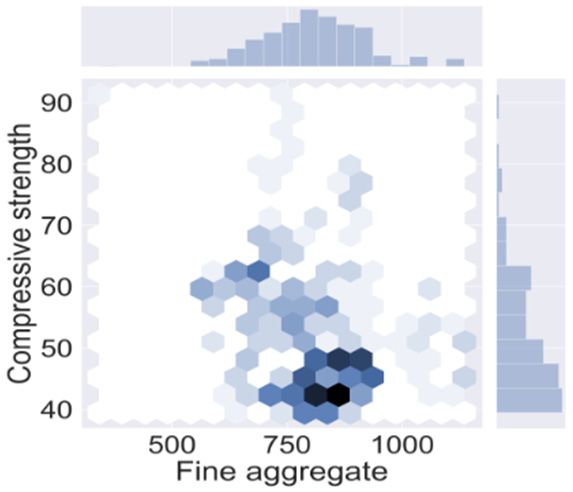
Appl. Sci. 2020, 10, 7330                                                                                            4 of 18

    Chromosomes in GEP consist of different arithmetic operations and a constant length variable.
An example of a GEP gene is shown in Equation (1):
Appl. Sci. 2020, 10, x FOR PEER REVIEW          √                                                                  4 of 18
                                           + .y. B.B. − . + .A.D.C.2.B.C.3                                              (1)

                                    +. . √set)
where A, B, C, D are variables (terminal    . and
                                               . −. +.
                                                    2, 3. are
                                                            . constants.
                                                              . 2. . . 3                                             (1)
 where A, B, C, D are variables (terminal set) and 2, 3 are constants.
3. Experimental Database Representation
 3. Experimental Database Representation
3.1. Dataset Used in Modeling Aspect
 3.1. Dataset
      Model Used      in Modeling
               evaluation           Aspect
                             is based    on data sample and the number of parameters used. A total of 357
datasets   wereevaluation
       Model      obtained from     published
                             is based    on dataliterature   (Seethe
                                                    sample and     Table  S1). These
                                                                      number           points were
                                                                                of parameters         trained,
                                                                                                  used.  A totalvalidated,
                                                                                                                   of 357
and   tested   during    modeling     to  build   a numerical-based      empirical   relation   for HSC.
 datasets were obtained from published literature (See Table S1). These points were trained, validated,     This   is done
to minimize
 and             the over
       tested during        fitting to
                         modeling    of build
                                         data in    machine learning
                                                 a numerical-based       approaches.
                                                                      empirical   relationThe
                                                                                            forsamples
                                                                                                 HSC. This were   divided
                                                                                                              is done    to
into  70/15/15   sets  to give  adamant     correlation   coefficient.  Behnood    et al. [54] predict
 minimize the over fitting of data in machine learning approaches. The samples were divided into         the mechanical
properties
 70/15/15 setsof concrete     with data
                   to give adamant          taken from
                                         correlation       published
                                                       coefficient.     literature.
                                                                     Behnood    et al. The
                                                                                        [54] samples    were
                                                                                              predict the       randomly
                                                                                                            mechanical
distributed    for  training  (70%),   validation    (15%),  and  testing  (15%)  sets.  Similarly,
 properties of concrete with data taken from published literature. The samples were randomly         Getahun     et al. [55]
forecasted
 distributedthe formechanical    properties
                    training (70%),            of concrete
                                       validation    (15%), by
                                                            anddistributing
                                                                 testing (15%)thesets.
                                                                                  dataSimilarly,
                                                                                        in the same    way aset
                                                                                                    Getahun     discussed.
                                                                                                                  al. [55]
Training   is usually   done  to  train the  model    with given  values   which  then   predict
 forecasted the mechanical properties of concrete by distributing the data in the same way        the  values  of strength
                                                                                                                        as
of unknownTraining
 discussed.      values, is
                          namely
                            usuallythe   testtoset.
                                      done      train the model with given values which then predict the values
 of strength of unknown values, namely the test set.
3.2. Programming-Based Presentation of Datasets
     Anaconda-based python version (version 3.7) programming [46] has been adopted to depict
the influence of various input parameters upon the mechanical strength of HSC. Compressive strength
of concrete is influenced by the number of parameters used in experimental work. Thus, cement
content (Type 1), water, superplasticizer (polycarboxylate), and fine and coarse aggregate (20 mm)
were used in modeling of the compressive strength of HSC. The impact of these input parameters was
visualized with the use of python which is done in Jupitar notebook [56] as shown in Figure 1.

                     (a)                                   (b)                                      (c)

                    (d)                                    (e)                                      (f)
             1. Hex
           Figure
      Figure      1. contour   graph
                     Hex contour     of input
                                   graph       parameters;
                                           of input           (a) Cement;
                                                    parameters;            (b) Coarse
                                                                   (a) Cement;        aggregate;
                                                                                (b) Coarse       (c) Fine
                                                                                           aggregate;      aggregate;
                                                                                                       (c) Fine
                       aggregate;
      (d) Super plasticizer;       (d) Super
                             (e) Water;        plasticizer; strength.
                                        (f) Compressive     (e) Water; (f) Compressive strength.

    Figure 1 represents the quantities which have adamant influence on the mechanical properties
of HSC. The darkish region shows the optimal/maximum concentration of variables as depicted in
Figure 1. Python is an effective machine learning approach that enables users to have a deep
understanding of the parameters that alter the functioning of the model. Python uses the seaborn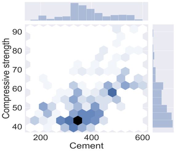
Appl. Sci. 2020, 10, 7330                                                                                       5 of 18

     Figure 1 represents the quantities which have adamant influence on the mechanical properties
of HSC. The darkish region shows the optimal/maximum concentration of variables as depicted
in Figure 1. Python is an effective machine learning approach that enables users to have a deep
understanding of the parameters that alter the functioning of the model. Python uses the seaborn
command to plot the correlation among the desired parameters. The description of the data variables
(see Table 2) used in the model consist of training set, validation set, and testing set as represented in
Tables 3–5. The parameters that define and ensure that optimum results are achieved for all techniques.
Identifying these parameters is of core importance.

                        Table 2. Statistical description of all data points used in model (Kg/m3 ).

                                                         Fine/Coarse
              Parameters               Cement                                 Water          Superplasticizer
                                                          Aggregate
                Mean                    384.34               0.96             173.56                   2.34
           Standard Error                4.92                0.01               0.82                   0.14
               Median                    360                 0.92               170                    1.25
                Mode                     360                 1.01               170                      1
         Standard Deviation             93.00                0.26              15.56                   2.69
          Sample Variance              8650.50               0.06             242.19                   7.24
               Kurtosis                  0.36                6.45              15.59                   2.88
              Skewness                   0.14                2.12               2.45                   1.79
                Range                    440                 1.86             170.08                    12
             Minimum                     160                 0.23               132                      0
             Maximum                     600                  2.1             302.08                    12
                 Sum                  137,212.84            344.07           61,963.8                 837.61
                Count                    357                 357                357                    357

                  Table 3. Statistical description of training data points used in the model (Kg/m3 ).

                                                         Fine/Coarse
              Parameters               Cement                                 Water          Superplasticizer
                                                          Aggregate
                Mean                    383.29               0.97             173.72                   2.42
           Standard Error                6.06                0.01               1.08                   0.17
               Median                    360                 0.92               170                    1.37
                Mode                     320                 1.01               170                      1
         Standard Deviation             95.95                0.27              17.17                   2.74
          Sample Variance              9206.57               0.07             295.07                   7.54
               Kurtosis                  0.60                5.82              14.42                   2.96
              Skewness                   0.19                2.08               2.48                   1.82
                Range                    420                 1.86             170.08                    12
             Minimum                     180                 0.23               132                      0
             Maximum                     600                  2.1             302.08                    12
                 Sum                   95,823.1             242.79           43,431.75                606.43
                Count                    250                 250                250                    250

                   Table 4. Statistical description of testing data points used in the model (Kg/m3 ).

                                                         Fine/Coarse
              Parameters               Cement                                 Water          Superplasticizer
                                                          aggregate
                Mean                    387.04               0.92             172.18                   1.98
           Standard Error               12.46                0.02               1.34                   0.33
               Median                    400                 0.90               170                      1
                Mode                     360                 0.75               170                      1
         Standard Deviation             95.76                0.18              10.35                   2.55
          Sample Variance              9170.56               0.03             107.25                   6.55
               Kurtosis                  0.22                6.82              0.18                    4.75
              Skewness                   0.17                1.66              0.33                    2.19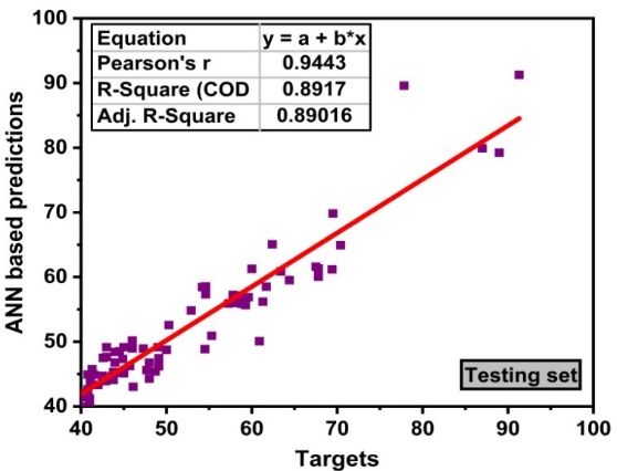
Appl. Sci. 2020, 10, 7330                                                                                        6 of 18

                                                         Table 4. Cont.

                                                            Fine/Coarse
              Parameters                 Cement                                 Water         Superplasticizer
                                                             aggregate
               Range                       440                 1.22              45.2                  12
              Minimum                      160                  0.58             154.8                 0
              Maximum                      600                  1.80              200                  12
                Sum                     22,835.54              54.38           10,159.18             117.09
               Count                       54                    54                54                  54

                  Table 5. Statistical description of validate data points used in the model (Kg/m3 ).

                                                            Fine/Coarse
              Parameters                 Cement                                 Water         Superplasticizer
                                                             Aggregate
                Mean                      390.52               0.90             173.07                2.10
           Standard Error                 12.58                 0.02              1.21                0.34
               Median                      378                  0.90              175                  1
                Mode                       360                  1.04              180                 0.5
         Standard Deviation               89.86                 0.15              8.67                2.47
          Sample Variance                8076.29                0.02             75.21                6.11
               Kurtosis                    1.08                 0.52            −0.18                 2.17
              Skewness                     0.17                 0.61            −0.62                 1.65
                Range                      440                 0.73              38.32                10.5
             Minimum                       160                  0.66              154                  0
             Maximum                       600                  1.39            192.32                10.5
                 Sum                    19,916.87              46.34            8826.8               107.57
                Count                       55                   55                55                  55

4. GEP Model Development
       The secondary objective during this research work was to derive a generalized equation for
the compressive strength of HSC. For this purpose, a terminal set, a function set, and four parameters
(d0 : cement content, d1 : fine to coarse aggregate, d2 : water, d3 : superplasticizer) were used in modeling.
These input parameters were utilized for the development of the model based on gene expression
programming. In addition, simple mathematical operations (+, −, /, ×) were used which were part of
the function set. A simple arithmetic operation was used to build an empirical-based relation which is
the function of the following parameters
                                                                                                 !
                                                         f ine
                            f 0 c = f cement content,          aggregate, water, superplasticizer                   (2)
                                                        coarse

     The GEP-based model, like all genetic algorithm models, is significantly influenced by the input
parameters (variables) upon which they are modeled. These variables had a substantial impact on
the generalizing fitness of these models. The variables used during this study are tabulated in Table 6.
The model time is an important parameter to analyze the effectiveness of the model. Thus, efforts shall
be made while selecting the sets which control the model time to ensure that the generalized model
always developed within due time. The selecting of these parameters is based on hit and trial method
to get maximum correlation. Root mean squared error (RMSE) was adopted in modeling. Moreover,
the performance of the model based on GEP is expressed by tree like architecture structures. This
structure consists of head size and number of genes [57].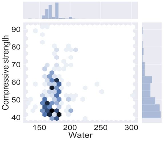
Appl. Sci. 2020, 10, 7330                                                                          7 of 18

              Table 6. Input parameters assigned in the gene expression programming (GEP) model.

                                       Parameters                            Settings
                                        General                                  fc0
                                         Genes                                   4
                                     Chromosomes                                 30
                                    Linking function                         Addition
                                       Head size                                 10
                                      Function set                           +, −, ×, ÷
                                             Numerical constants
                                   Constant per gene                           10
                                     Lower bound                              −10
                                      Data type                        Floating number
                                     Upper bound                              10
                                   Genetic Operators
                              Two-point recombination rate                    0.00277
                                 Gene transposition rate                      0.00277

5. Model Performance Analysis
    To assess the viability of any model and to evaluate its performance, various indicators have been
used. Each indicator has its method of inferring the performance of these models. The indicators
commonly used include root mean squared error (RMSE), mean absolute error (MAE), relative mean
square error (RSE), relative root mean squared error (RRMSE), and coefficient of determination (R2 ).
The mathematical expressions for these indicators are given below.
                                                    s
                                                               (exi − moi )2
                                                        Pn
                                                         i=1
                                       RMSE =                                                         (3)
                                                                 n
                                                    Pn
                                                        i=1 |exi   − moi |
                                          MAE =                                                       (4)
                                                               n
                                                             (moi− exi )2
                                                    Pn
                                          RSE = Pi=1               2
                                                                                                      (5)
                                                 n
                                                   i=1 (ex − exi )
                                                 s
                                                    Pn                  2
                                               1       i=1 (exi − moi )
                                   RRMSE =                                                            (6)
                                               e              n
                                        Pn
                                          i=1 (exi − exi )(moi − moi )
                                 R= q                                                                 (7)
                                      Pn                2 Pn                 2
                                       i=1 (exi − exi )     i=1 (moi − moi )

                                                        RRMSE
                                                  ρ=                                                  (8)
                                                         1+R
where:
     exi = experimental actual strength.
     moi = model strength.
     ex i = average value of the experimental outcome.
     moi = average value of the predicted outcome.
     In this paper, the performance of the model is also evaluated by using the coefficient of
determination (R2 ). The model is deemed effective when the value of R2 is greater than 0.8 and is
close to 1 [58]. The value obtained through model is the reflection that shows the correlation between
the experimental and predicted outcomes. Lower values of the indicator errors like MAE, RRMSE,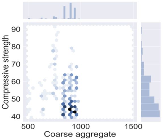
Appl. Sci. 2020, 10, 7330                                                                                                  8 of 18

RMSE, and RSE indicate higher performance. Machine learning is a good approach in the prediction
of properties. However, overfitting issues in a dataset have a malignant effect in validation and
fore casting of mechanical aspect of HSC. Thus, overcoming this problem of overfitting has become
a dire need in supervised machine learning algorithms. Researchers used objective function (OBF) for
the accuracy of models. OBF uses overall data samples along with the error and regression coefficient.
This then provides a more accurate generalized model with adamant higher accuracy and is represented
in Equation (8) [59].
                                              n      − nTest              nTest
                                       OBF = h Train         iρTrain + 2(       )ρTest             (9)
      Appl. Sci. 2020, 10, x FOR PEER REVIEW         n                     n               8 of 18

6. Results andand
     6. Results Discussion
                   Discussion

6.1. Random   Forest
      6.1. Random    Model
                  Forest   Analysis
                         Model Analysis
      RandomRandom forest   is an
                        forest     ensemble
                                is an ensemblemodeling
                                                  modeling algorithm        whichuses
                                                              algorithm which        uses    a weak
                                                                                         a weak        learner
                                                                                                    learner     to give
                                                                                                            to give       the best
                                                                                                                    the best
performance
      performanceas depicted     in Figure
                       as depicted           2. These
                                       in Figure       algorithms
                                                   2. These           are supervised
                                                               algorithms                 learners
                                                                             are supervised           giving
                                                                                                 learners     adamant
                                                                                                           giving        accuracy
                                                                                                                   adamant
      accuracy
in terms          in terms ofThe
           of correlation.        correlation.
                                     model isThe     modelinto
                                                 divided      is divided
                                                                 twenty into     twenty to
                                                                           submodels       submodels     to give maximum
                                                                                               give maximum       determination
      determination      of  coefficient  as illustrated in   Figure  2a.  It  can be  seen   that
of coefficient as illustrated in Figure 2a. It can be seen that sub-model equal to 10 outbursts     sub-model   equal to
                                                                                                                       and 10gives
      outbursts    and   gives a  strong  relationship. It is due  to incorporation     of a  weak   learner
a strong relationship. It is due to incorporation of a weak learner (decision tree), which then uses it in   (decision tree),
      which then uses it in the ensembling algorithm. Moreover, the model gives an obstinate                     correlation
the ensembling       algorithm. Moreover, the model gives an obstinate correlation of R2 = 0.96 between
      of R2 = 0.96 between experimental and predicted values and gives good validation results as
experimental and predicted values and gives good validation results as illustrated in Figure 2b,c. In
      illustrated in Figure 2b and Figure 2c. In addition, the model performance shows less error as
addition,    the model
      illustrated           performance
                    in Figure    2d. All the shows    less
                                              predicted     error
                                                         data      as illustrated
                                                                points                in Figure
                                                                        lie in the same     range 2d.    All the predicted
                                                                                                    of experimental  values data
points   lie an
      with   in error
                the same      range
                       less than      of experimental
                                   10MPa.   This shows thatvalues    with an
                                                               the random        error
                                                                              forest    less than
                                                                                     ensemble         10MPa.
                                                                                                  algorithm    This
                                                                                                             gives   shows that
                                                                                                                   adamant
the random      forest ensemble algorithm gives adamant good results.
      good results.

                                   (a)                                                     (b)

                                   (c)                                                     (d)

      FigureFigure  2. Model
               2. Model       evaluation
                          evaluation    (a)(a)Ensemble
                                               Ensemblemodel
                                                          model withwith2020submodels; (b)(b)
                                                                              submodels;   validation based
                                                                                              validation    on RF;
                                                                                                          based on(c)
                                                                                                                   RF; (c)
            testing
      testing  basedbased on RF;
                       on RF; (d) (d) error
                                   error     distributionofofthe
                                         distribution         the testing
                                                                   testing set.
                                                                           set.

           Statistical analysis checks are applied to check the model performance using random forest. This
      is an indirect method which shows model performance. These statistical analyses check the errors in
      the model; thus, RMSE, MAE, RSE, and RRMSE are used as shown in Table 7. The RF model is
      ensemble one and thus shows lesser error in the prediction aspect.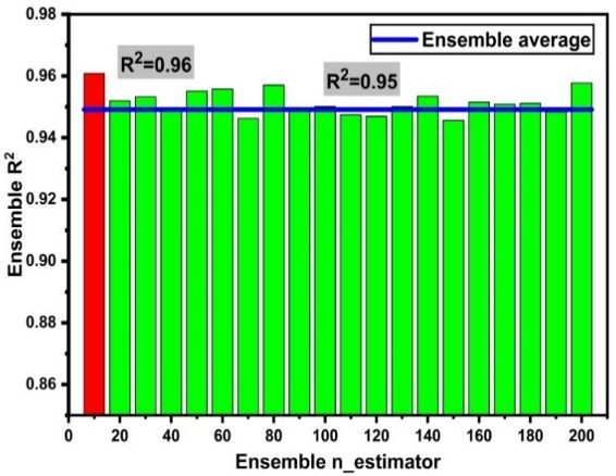
Appl. Sci. 2020, 10, 7330 9 of 18
Statistical analysis checks are applied to check the model performance using random forest. This
is an indirect method which shows model performance. These statistical analyses check the errors
in the model; thus, RMSE, MAE, RSE, and RRMSE are used as shown in Table 7. The RF model is
ensemble one and thus shows lesser error in the prediction aspect.
Table 7. Random forest (RF) statistical analysis.
Model RMSE MAE R2
Validation Testing Validation Testing Validation Testing
1.22 1.42 0.475 0.495 0.967 0.041
Fc RRMSE RSE P(row)
Validation Testing Validation Testing Validation Testing
0.0186 0.021 0.072 0.053 0.024 0.025
6.2. Empirical Relation of HSC Using the GEP Model
Gene expression programming is an individual supervised machine learning approach which
predicts the mechanical compressive strength using tree-based expression. Moreover, GEP gives
an empirical relation with input parameters as shown in Equation (9). This simplified equation is
then used to predict the compressive strength of HSC. This equation comes from the expression tree
which used a function set and terminal set with the mathematics operator as shown in Figure 3. It
shows the relationship between input parameters and output strength. GEP utilizes linear as well as
non-linear algorithms in the forecasting of mechanical properties.
fc (MPa) = A + B + C (10)
where !
19.97 ∗ cement
A= (11)
(water + superplasticizer) + 15.31
+
− 0.58 + superplasticizer
F agg F
C
B = (−5.32 + (−2.41)) − ∗ agg (12)
−0.50 C
+
−4.77
C= −0.77 ∗ ∗ ((water + superplasticizer) ∗ 8.64) + superplasticizer (13)
cement + 32.4
Before running the GEP algorithm, the procedure starts with the selection of the number of
chromosomes and basic operators that are provided by GEP software. The model uses hit and trial
techniques where chromosomes of varying sizes and gene numbers are used with operational operators,
thus ensuring the selection of the best model. The selected model has the best/fittest gene available
within the population which gives adamant performance in making the model. The most feasible
and desirable outcome used in the GEP model is fc , which is expressed in the form of an expression
tree as shown in Figure 3. Expression tree uses a linkage function with a basic mathematical operator
with some constants. It is worth mentioning here that the GEP algorithm uses the RMSE function for
its prediction.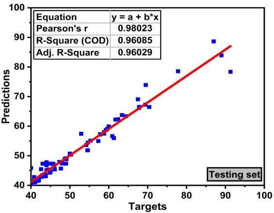
Appl. Sci. 2020, 10, 7330 10 of 18
Appl. Sci. 2020, 10, x FOR PEER REVIEW 10 of 18
Figure 3.
Figure Expression tree
3. Expression tree of
of high
high strength
strength concrete
concrete (HSC)
(HSC) using
using gene
gene expression.
expression.
6.3. GEP Model Evaluation
Before running the GEP algorithm, the procedure starts with the selection of the number of
Model evaluation
chromosomes and basicand its representation
operators between
that are provided byobserved and predicted
GEP software. The model values
usesishitillustrated
and trial
in Figure 4. where
techniques GEP-based machine learning
chromosomes of varyingalgorithm
sizes and is an effective
gene approach
numbers to assess
are used with the strength
operational
parameters of HSC.
operators, thus Model
ensuring theassessment
selection ofinthe
machine learning
best model. Theisselected
usually model
done with regression
has the analysis.
best/fittest gene
Regression
available analysis
within theshows the accuracy
population of anyadamant
which gives model with value close
performance in to one is the
making an adamant
model. The accurate
most
model asand
feasible represented
desirableinoutcome
Figure 4b. It shows
used in thethat
GEPthe regression
model is ,line of the
which testing andinvalidation
is expressed the form sets is
of an
close to 1. Figure
expression 4a,b
tree as represent
shown the regression
in Figure analysis tree
3. Expression of validation and testing
uses a linkage sets with
function with coefficient
a basic
of determination
mathematical R2 . This
operator withvalue
someisconstants.
greater than
It is 0.8 which
worth depicts the
mentioning hereaccuracy
that the of
GEPthealgorithm
model as uses 0.91
andRMSE
the 0.90 for the testing
function (see
for its Figure 4a) and validation (see Figure 4b) sets, respectively. Normalization
prediction.
of gathered data from published literature was also done within the range of zero and one to show
6.3. GEP Model Evaluation
the accurateness of data as illustrated in Figure 4c.
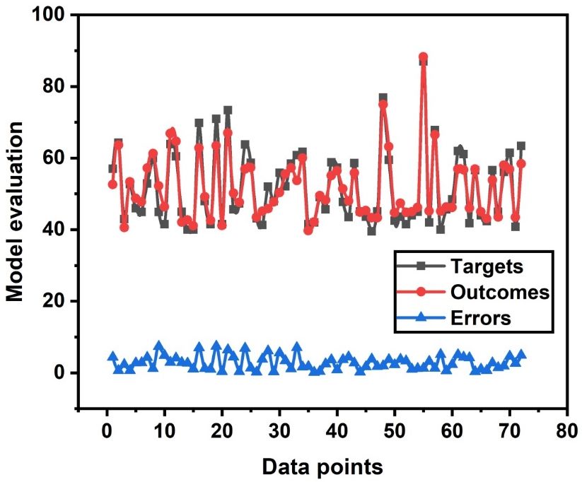
Model evaluation and its representation between observed and predicted values is illustrated in
Figure 4. GEP-based machine learning algorithm is an effective approach to assess the strength
parameters of HSC. Model assessment in machine learning is usually done with regression analysis.
Regression analysis shows the accuracy of any model with value close to one is an adamant accurate
model as represented in Figure 4(b). It shows that the regression line of the testing and validation sets
is close to 1. Figure 4(a) and Figure 4(b) represent the regression analysis of validation and testing
sets with coefficient of determination R2. This value is greater than 0.8 which depicts the accuracy ofAppl. Sci. 2020, 10, x FOR PEER REVIEW 11 of 18
the model as 0.91 and 0.90 for the testing (see Figure 4(a)) and validation (see Figure 4(b)) sets,
respectively.
Appl. Sci. 2020, 10,Normalization
7330 of gathered data from published literature was also done within
11 ofthe
18
range of zero and one to show the accurateness of data as illustrated in Figure 4(c).
(a) (b)
(c)
Figure 4. Model evaluation (a) Validation results of data based on GEP; (b) testing results of data; (c)
Figure 4.
normalized
normalized range
range of
of data.
data.
Statistical
Statistical measures
measures areare used
used to
to evaluate
evaluate the
the performance
performance of of the
the model
model byby using
using MAE,
MAE, RRMSE,
RRMSE,
RSE,
RSE, and
and RMSE
RMSE as as done
done similarly
similarly in
in aa random
random forest
forest model
model asas shown
shown inin Table
Table 8.
8. Low
Low error
error and
and higher
higher
coefficient 2
coefficientgive
givebetter
betterperformance
performanceof ofthe
themodel.
model.Most
Mostofofthe
theerrors
errorslies
liesbelow
below55MPa
MPawith
withan anRR2 value
value
greater than 0.8. Thus, it depicts the accuracy of the finalized model. Further analysis
greater than 0.8. Thus, it depicts the accuracy of the finalized model. Further analysis is alsois also performed
to evaluate to
performed theevaluate
performance of the modelofby
the performance thedetermining the standard
model by determining deviation
the standard(SD) and covariance
deviation (SD) and
(COV). The values of SD and COV are determined to be 0.16 and 0.059, respectively.
covariance (COV). The values of SD and COV are determined to be 0.16 and 0.059, respectively.
Table 8. Statistical
Table 8. Statistical calculations
calculations of
of the
the proposed
proposed model.
model.
Model
Model RMSE RMSE MAE
MAE RSERSE
Validation
Validation Testing
Testing Validation
Validation Testing
Testing Validation Validation
Testing Testing
1.42 1.62 0.575 0.595 0.092 0.023
1.42 1.62 0.575 0.595 0.092 0.023
Fc RRMSE R P(row)
Fc RRMSETesting
Validation R
Validation Testing P(row)
Validation Testing
0.0286
Validation 0.031
Testing Validation0.957 Testing
0.031 Validation 0.014 Testing 0.015
The accuracy0.0286
and performance 0.031of the machine
0.957 learning-based
0.031 model is0.014
evaluated by 0.015
conducting
error distribution between actual targets and predicted values of the testing set as shown in Figure 5.
It can
Thebeaccuracy
seen thatandtheperformance
model predicted
of the the outcome
machine nearly or equal
learning-based modeltois the experimental
evaluated values.
by conducting
Moreover,
error the error
distribution distribution
between actual of the testing
targets set shows
and predicted that 86%
values oftesting
of the the datasetsample liesin
as shown below 5 MPa
Figure 5. It
andbe
can 13.88% of the
seen that thedata
modelliespredicted
in the range of 5 MPa
the outcome to 8 MPa
nearly withto7.47
or equal MPa as maximum
the experimental values.error. Thus,
Moreover,
the error
the GEP-based model
distribution of not only gives
the testing obstinate
set shows that accuracy
86% of theindata
terms of correlation
sample lies below but
5 MPaalso gives
and the
13.88%
of the data lies in the range of 5 MPa to 8 MPa with 7.47 MPa as maximum error. Thus, the GEP-based
model not only gives obstinate accuracy in terms of correlation but also gives the empirical equationAppl. Sci. 2020, 10, 7330 12 of 18
Appl. Sci. 2020, 10, x FOR PEER REVIEW 12 of 18
shown in Equation (9). This equation will help the users to predict the compressive strength of concrete
empirical
by equation
using hand shown in Equation (9). This equation will help the users to predict the
calculations.
compressive strength of concrete by using hand calculations.
Figure
Figure 5. Distribution of
5. Distribution of data
data with
with error
error range.
range.
7. Statistical Analysis Checks on RF and GEP Model
7. Statistical Analysis Checks on RF and GEP Model
The accuracy of any model is based on data points. The higher the points, the greater will be
The accuracy of any model is based on data points. The higher the points, the greater will be the
the accuracy of the entire model [60]. Frank et al. [60] present an ideal solution based on the ratio of
accuracy of the entire model [60]. Frank et al. [60] present an ideal solution based on the ratio of input
input data samples to its parameters involved. This ratio should be equal to or greater than three for
data samples to its parameters involved. This ratio should be equal to or greater than three for good
good performance of the model. This study uses 357 data samples with the 4 variables mentioned
performance of the model. This study uses 357 data samples with the 4 variables mentioned earlier
earlier with the ratio equal to 89.25. This ratio value is exceptionally higher, indicating the accuracy
with the ratio equal to 89.25. This ratio value is exceptionally higher, indicating the accuracy of the
of the model. Farjad et al. [33] used a similar approach to validate the model and yield adamant
model. Farjad et al. [33] used a similar approach to validate the model and yield adamant results with
results with a ratio greater than 3. Researchers suggest different approaches for the validation of
a ratio greater than 3. Researchers suggest different approaches for the validation of a model using
a model using external statistical measures [61,62]. Golbraikh et al. [62] validate their model using
external statistical measures [61,62]. Golbraikh et al. [62] validate their model using the slope of the
the slope of the regression line (k’ or k) of the model. This line measures the accuracy of the model by
regression line (k’ or k) of the model. This line measures the accuracy of the model by using
using experimental and predicted values. Any value greater than 0.8 or close to 1 will yield obstinate
experimental and predicted values. Any value greater than 0.8 or close to 1 will yield obstinate
performance of the model [61]. All these external checks have been presented in tabulated in Table 9.
performance of the model [61]. All these external checks have been presented in tabulated in Table 9.
Table 9. Statistical analysis of RF and GEP models from external validation.
Table 9. Statistical analysis of RF and GEP models from external validation.
S.No Equation Condition RF Model GEP Model
S.No Equation
Pn Condition RF Model GEP Model
(e ×m )
1 k = i=1 2i i 0.85 < k < 1.15 0.99 0.98
Pn ei
i=1 (ei ×mi )
2 k0 = 0.85 < k < 1.15 1.00 1.00
1 ∑ (m2i
× ) 0.85 < < 1.15 0.99 0.98
=
Pn 2
i=1 ( mi −eoi)
3 R2o − , eo = k × m i
o 2
R2o 1 0.99 0.97
) i
Pn
(i=1 mi −mi
(∑ )( o× 0 )
Pn 2
2 4
0
Ro2 i=1 ei −moi 2 1<
R0.85 < 1.15
0.99 1.00 0.991.00
−
′=(
Pn
i=1
o 2
ei −ei)
, m i = k × ei o
3 ∑ ( − ) ≅1 0.99 0.97
8. Comparison−of Models with ANN, and=Decision
× Tree
∑ ( − )
Ensemble RF and GEP approach are compared with other supervised machine learning algorithms,
∑ ( −
4 ANN and DT as depicted ) ≅1 0.99 0.99
namely − , Figure
in = ′6.× These techniques, along with GEP, are individual
∑ (RF −
algorithms. However, is an )ensemble one which incorporates a base learner as an individual
learner and model it with bagging technique to give an adamant strong correlation. It should be kept
8. Comparison of Models with ANN and Decision Tree
Ensemble RF and GEP approach are compared with other supervised machine learning
algorithms, namely ANN and DT as depicted in Figure 6. These techniques, along with GEP, areAppl. Sci. 2020, 10, x FOR PEER REVIEW 13 of 18
Appl. Sci. 2020, 10, 7330 13 of 18
individual algorithms. However, RF is an ensemble one which incorporates a base learner as an
individual learner and model it with bagging technique to give an adamant strong correlation. It
in mindbe
should that
keptallin
models are based
mind that on python
all models (anaconda).
are based on pythonThe comparison
(anaconda). Theofcomparison
models is presented
of models
in Figure 6. The RF outburst in performance of the model can be seen with R 2 = 0.96 and its error
is presented in Figure 6. The RF outburst in performance of the model can be seen with R2=0.96 and
distribution as shownasinshown
its error distribution Figurein6a,b.
Figure Whereas
6(a) andindividual models
Figure 6(b). WhereasANN, DT, andmodels
individual GEP showANN, good
DT,
response with R 2 = 0.89, 0.90, and 0.90, respectively. Figure 6d represents the error distribution of
and GEP show good response with R = 0.89, 0.90, and 0.90, respectively. Figure 6(d) represents the
2
decision tree with maximum error below 10 MPa. However, 18.19 MPa
error distribution of decision tree with maximum error below 10 MPa. However, 18.19 MPa isis reported as the maximum
error. A similar
reported as the trend
maximum has also been
error. A observed for ANN
similar trend andbeen
has also GEP observed
models with maximum
for ANN errormodels
and GEP values
of 11.80 MPa and 7.48 MPa, respectively as shown in Figure 6f,h. Moreover,
with maximum error values of 11.80 MPa and 7.48 MPa, respectively as shown in Figure 6(f) and researchers used different
algorithm-based machine
Figure 6(h). Moreover, learning used
researchers techniques foralgorithm-based
different the prediction ofmachine
mechanical properties
learning of high
techniques for
strength concrete. Ahmed et al. [63] used an ANN algorithm and forecasted the
the prediction of mechanical properties of high strength concrete. Ahmed et al. [63] used an ANN mechanical properties
(slump
algorithmandand
compressive
forecastedstrength) of HSC.properties
the mechanical The author evaluated
(slump its model with
and compressive ANN and
strength) revealed
of HSC. The
strong
authorcorrelation
evaluated for slump with
its model and compressive of aboutstrong
ANN and revealed 0.99. Singh et al. [64]
correlation forecasted
for slump and the mechanical
compressive of
properties of HSC by using RF and M5P algorithms and reported strong correlation
about 0.99. Singh et al. [64] forecasted the mechanical properties of HSC by using RF and M5P for the testing set
of 0.876 andand
algorithms 0.814, respectively.
reported strong correlation for the testing set of 0.876 and 0.814, respectively.
(a) (b)
(c) (d)
(e) (f)
Figure 6. Cont.Appl. Sci. 2020, 10, 7330 14 of 18
Appl. Sci. 2020, 10, x FOR PEER REVIEW 14 of 18
Appl. Sci. 2020, 10, x FOR PEER REVIEW 14 of 18
(g) (h)
(g) (h)
Figure 6. Model evaluation with errors (a) RF regression analysis; (b) error distribution based on the RF
Figure 6. Model
Figure evaluation
6. Model withwith
evaluation errors (a) (a)
errors RF RF
regression
regressionanalysis; (b)
analysis; (b)error
errordistribution
distributionbased
based on the RF
on the RF
model; (c) decision tree (DT) regression analysis; (d) error distribution based on DT; (e) artificial neural
model; (c) decision
model; tree tree
(c) decision (DT)(DT)
regression analysis;
regression (d)(d)
analysis; error distribution
error distributionbased
basedononDT;
DT; (e)
(e) artificial neural
artificial neural
network (ANN) regression analysis; (f) error distribution based on ANN; (g) GEP regression analysis; (h)
network (ANN)
network regression
(ANN) analysis;
regression (f) error
analysis; distribution
(f) error based
distribution on ANN;
based on ANN;(g) GEP regression
(g) GEP regressionanalysis; (h)
analysis;
error distribution based on GEP.
error(h)
distribution based on GEP.
error distribution based on GEP.
9. Permutation
9.
9. Permutation Feature
Permutation Feature Analysis
Feature Analysis (PFA)
Analysis (PFA)
(PFA)
Permutation feature
Permutation
Permutation feature analysis
feature analysis (PFA)
analysis (PFA) is
(PFA) isperformed
is performed to
performed todetermine
to determine the
determine themost
the mostinfluential
most influentialparameters
influential parameters
parameters
affecting the
affecting
affecting the compressive
the compressive strength
compressive strength of
strength of HSC.
of HSC. PFA
HSC. PFA isis
PFA is performed
performed by
performed by utilizing
by utilizing an
utilizing an extension
an extension of
extension of python
of python
python
programming.
programming. Figure
Figure 77 shows
shows the
the results
results of
of PFA.
PFA. The
The results
results show
show that
that all
all the
the
programming. Figure 7 shows the results of PFA. The results show that all the variables consideredvariables
variables considered
considered
in this
in
in this study
this study strongly
study strongly affect
strongly affect the
affect the compressive
the compressive strength
compressive strength property
strength property of
property of HSC.
of HSC. However,
HSC. However, the
However, the effect
the effect of
effect of super
of super
super
plastizeris
plastizer
plastizer ismore
is moreas
more ascompared
as comparedto
compared tothe
to theother
the othervariables.
other variables.
variables.
(a)
(a) (b)
(b)
Figure 7.
Figure 7. Permutation
Permutation analysis
analysis of
of input
input variables
variables (a)
(a) model
model base
base (b)
(b) contribution
contributionof
ofinput
inputvariables.
variables.
Figure 7. Permutation analysis of input variables (a) model base (b) contribution of input variables.
10.
10. Conclusions
Conclusions
10. Conclusions
Supervised
Supervised machine
machine learning
learning predicts
predicts the
the mechanical
mechanical properties
properties of
of concrete
concrete and
and gives
givesoutmost
outmost
Supervised
result. This will machine
help the learning
user to predicts
forecast the the mechanical
desire propertiesproperties
rather of
than concrete
conductingand
thegives outmost
experimental
result. This
result. The
This will help
will help the user
the user to forecast the desire properties rather than conducting the
setup.
experimental following
setup. properties
The areto
following
forecast
deduced
properties
theusing
from desire
are theproperties
machine
deduced from
rather algorithm.
learning
using
than conducting the
the machine learning
experimental setup. The following properties are deduced from using the machine learning
algorithm.
1. Random forest is an ensemble approach which gives adamant performance between observed
algorithm.
1. and predicted
Random forestvalue.
is an It is due to
an ensemble
ensemble incorporation
approach whichof a weak
gives learner
adamant as base learner
performance (decision
between tree)
observed
1. Random forest is approach which gives adamant performance between observed
and
and gives determination
predicted value. It isofdue
It is coefficient
due R = 0.96.of a weak learner as base learner (decision tree)
2
to incorporation
incorporation
and predicted value. to of a weak learner as base learner (decision tree)
and gives determination of coefficient R 2 = 0.96.
and gives determination of coefficient R = 0.96.
2Appl. Sci. 2020, 10, 7330 15 of 18
2. GEP is an individual model rather than an ensemble algorithm. It gives a good relation with
the empirical relation. This relation can be used to predict the mechanical aspect of high strength
concrete via hand calculation.
3. Comparison of the RF and GEP models is made with ANN and DT. However, RF outbursts
and gives an obstinate relation of R2 = 0.96. GEP model gives R2 = 0.90. ANN and DT models
give 0.89 and 0.90, respectively. Moreover, RF gives less errors as compared to others individual
algorithms. This is due to the bagging mechanism of RF.
4. Permutation features give an influential parameter in HSC. This help us to check and know
the most dominant variables in using experimental work; thus, all the variables have an effect on
compressive strength.
Supplementary Materials: The following are available online at http://www.mdpi.com/2076-3417/10/20/7330/s1,
Table S1: Supplementary material.
Author Contributions: F.F., software and investigation; M.N.A., writing—review and editing; K.K.,
writing—review and editing; M.R.S., review and editing; M.F.J., graphs and review; F.A., editing and writing;
R.A., funding and review. All authors have read and agreed to the published version of the manuscript.
Funding: This research received no external funding.
Acknowledgments: This research was supported by the Deanship of Scientific Research (DSR) at King Faisal
University (KFU) through “18th Annual Research Project No. 180062”. The authors wish to express their gratitude
for the financial support that has made this study possible and also supported by the deanship of scientific research
at Prince Sattam Bin Abdulaziz University under the research project number 2020/01/16810.
Conflicts of Interest: The authors declare no conflict of interest.
References
1. Zhang, X.; Han, J. The effect of ultra-fine admixture on the rheological property of cement paste. Cem. Concr.
Res. 2000, 30, 827–830. [CrossRef]
2. Khaloo, A.; Mobini, M.H.; Hosseini, P. Influence of different types of nano-SiO2 particles on properties of
high-performance concrete. Constr. Build. Mater. 2016, 113, 188–201. [CrossRef]
3. Hooton, R.D.; Bickley, J.A. Design for durability: The key to improving concrete sustainability. Constr. Build.
Mater. 2014, 67, 422–430. [CrossRef]
4. Farooq, F.; Akbar, A.; Khushnood, R.A.; Muhammad, W.L.B.; Rehman, S.K.U.; Javed, M.F. Experimental
investigation of hybrid carbon nanotubes and graphite nanoplatelets on rheology, shrinkage, mechanical,
and microstructure of SCCM. Materials 2020, 13, 230. [CrossRef]
5. Carrasquillo, R.; Nilson, A.; Slate, F.S. Properties of High Strength Concrete Subjectto Short-Term Loads.
1981. Available online: https://www.concrete.org/publications/internationalconcreteabstractsportal.aspx?m=
details&ID=6914 (accessed on 27 September 2020).
6. Mbessa, M.; Péra, J. Durability of high-strength concrete in ammonium sulfate solution. Cem. Concr. Res.
2001, 31, 1227–1231. [CrossRef]
7. Baykasoǧlu, A.; Öztaş, A.; Özbay, E. Prediction and multi-objective optimization of high-strength concrete
parameters via soft computing approaches. Expert Syst. Appl. 2009, 36, 6145–6155. [CrossRef]
8. Demir, F. Prediction of elastic modulus of normal and high strength concrete by artificial neural networks.
Constr. Build. Mater. 2008, 22, 1428–1435. [CrossRef]
9. Demir, F. A new way of prediction elastic modulus of normal and high strength concrete-fuzzy logic. Cem.
Concr. Res. 2005, 35, 1531–1538. [CrossRef]
10. Yan, K.; Shi, C. Prediction of elastic modulus of normal and high strength concrete by support vector machine.
Constr. Build. Mater. 2010, 24, 1479–1485. [CrossRef]
11. Ahmadi-Nedushan, B. Prediction of elastic modulus of normal and high strength concrete using ANFIS and
optimal nonlinear regression models. Constr. Build. Mater. 2012, 36, 665–673. [CrossRef]
12. Safiuddin, M.; Raman, S.N.; Salam, M.A.; Jumaat, M.Z. Modeling of compressive strength for
self-consolidating high-strength concrete incorporating palm oil fuel ash. Materials 2016, 9, 396. [CrossRef]
[PubMed]Appl. Sci. 2020, 10, 7330 16 of 18
13. Al-Shamiri, A.K.; Kim, J.H.; Yuan, T.F.; Yoon, Y.S. Modeling the compressive strength of high-strength
concrete: An extreme learning approach. Constr. Build. Mater. 2019, 208, 204–219. [CrossRef]
14. Aslam, F.; Farooq, F.; Amin, M.N.; Khan, K.; Waheed, A.; Akbar, A.; Javed, M.F.; Alyousef, R.; Alabdulijabbar, H.
Applications of Gene Expression Programming for Estimating Compressive Strength of High-Strength
Concrete. Adv. Civ. Eng. 2020, 2020, 1–23. [CrossRef]
15. Samui, P. Multivariate adaptive regression spline (MARS) for prediction of elastic modulus of jointed rock
mass. Geotech. Geol. Eng. 2013, 31, 249–253. [CrossRef]
16. Gholampour, A.; Mansouri, I.; Kisi, O.; Ozbakkaloglu, T. Evaluation of mechanical properties of concretes
containing coarse recycled concrete aggregates using multivariate adaptive regression splines (MARS), M5
model tree (M5Tree), and least squares support vector regression (LSSVR) models. Neural Comput. Appl.
2020, 32, 295–308. [CrossRef]
17. Shahmansouri, A.A.; Bengar, H.A.; Ghanbari, S. Compressive strength prediction of eco-efficient GGBS-based
geopolymer concrete using GEP method. J. Build. Eng. 2020, 31, 101326. [CrossRef]
18. Javed, M.F.; Farooq, F.; Memon, S.A.; Akbar, A.; Khan, M.A.; Aslam, F.; Alyousef, R.; Alabduljabbar, H.;
Rehman, S.K.U. New prediction model for the ultimate axial capacity of concrete-filled steel tubes: An
evolutionary approach. Crystals 2020, 10, 741. [CrossRef]
19. Sonebi, M.; Abdulkadir, C. Genetic programming based formulation for fresh and hardened properties of
self-compacting concrete containing pulverised fuel ash. Constr. Build. Mater. 2009, 23, 2614–2622. [CrossRef]
20. Rinchon, J.P.M. Strength durability-based design mix of self-compacting concrete with cementitious blend
using hybrid neural network-genetic algorithm. IPTEK J. Proc. Ser. 2017, 3. [CrossRef]
21. Kang, F.; Li, J.; Dai, J. Prediction of long-term temperature effect in structural health monitoring of concrete
dams using support vector machines with Jaya optimizer and salp swarm algorithms. Adv. Eng. Softw. 2019,
131, 60–76. [CrossRef]
22. Ling, H.; Qian, C.; Kang, W.; Liang, C.; Chen, H. Combination of support vector machine and K-fold cross
validation to predict compressive strength of concrete in marine environment. Constr. Build. Mater. 2019,
206, 355–363. [CrossRef]
23. Ababneh, A.; Alhassan, M.; Abu-Haifa, M. Predicting the contribution of recycled aggregate concrete to
the shear capacity of beams without transverse reinforcement using artificial neural networks. Case Stud.
Constr. Mater. 2020, 13, e00414. [CrossRef]
24. Xu, J.; Chen, Y.; Xie, T.; Zhao, X.; Xiong, B.; Chen, Z. Prediction of triaxial behavior of recycled aggregate
concrete using multivariable regression and artificial neural network techniques. Constr. Build. Mater. 2019,
226, 534–554. [CrossRef]
25. Van Dao, D.; Ly, H.B.; Vu, H.L.T.; Le, T.T.; Pham, B.T. Investigation and optimization of the C-ANN structure
in predicting the compressive strength of foamed concrete. Materials 2020, 13, 1072. [CrossRef]
26. Han, Q.; Gui, C.; Xu, J.; Lacidogna, G. A generalized method to predict the compressive strength of
high-performance concrete by improved random forest algorithm. Constr. Build. Mater. 2019, 226, 734–742.
[CrossRef]
27. Zounemat-Kermani, M.; Stephan, D.; Barjenbruch, M.; Hinkelmann, R. Ensemble data mining modeling in
corrosion of concrete sewer: A comparative study of network-based (MLPNN & RBFNN) and tree-based
(RF, CHAID, & CART) models. Adv. Eng. Inform. 2020, 43, 101030. [CrossRef]
28. Zhang, J.; Li, D.; Wang, Y. Toward intelligent construction: Prediction of mechanical properties of
manufactured-sand concrete using tree-based models. J. Clean. Prod. 2020, 258, 120665. [CrossRef]
29. Vakhshouri, B.; Nejadi, S. Predicition of compressive strength in light-weight self-compacting concrete by
ANFIS analytical model. Arch. Civ. Eng. 2015, 61, 53–72. [CrossRef]
30. Dutta, S.; Murthy, A.R.; Kim, D.; Samui, P. Prediction of Compressive Strength of Self-Compacting Concrete
Using Intelligent Computational Modeling Call for Chapter: Risk, Reliability and Sustainable Remediation
in the Field OF Civil AND Environmental Engineering (Elsevier) View project Ground Rub. 2017. Available
online: https://www.researchgate.net/publication/321700276 (accessed on 27 September 2020).
31. Vakhshouri, B.; Nejadi, S. Prediction of compressive strength of self-compacting concrete by ANFIS models.
Neurocomputing 2018, 280, 13–22. [CrossRef]
32. Info, A. Application of ANN and ANFIS Models Determining Compressive Strength of Concrete. Soft
Comput. Civ. Eng. 2018, 2, 62–70. Available online: http://www.jsoftcivil.com/article_51114.html (accessed on
27 September 2020).Appl. Sci. 2020, 10, 7330 17 of 18
33. Iqbal, M.F.; Liu, Q.f.; Azim, I.; Zhu, X.; Yang, J.; Javed, M.F.; Rauf, M. Prediction of mechanical properties of
green concrete incorporating waste foundry sand based on gene expression programming. J. Hazard. Mater.
2020, 384, 121322. [CrossRef]
34. Trtnik, G.; Kavčič, F.; Turk, G. Prediction of concrete strength using ultrasonic pulse velocity and artificial
neural networks. Ultrasonics 2009, 49, 53–60. [CrossRef] [PubMed]
35. Shahmansouri, A.A.; Yazdani, M.; Ghanbari, S.; Bengar, H.A.; Jafari, A.; Ghatte, H.F. Artificial neural network
model to predict the compressive strength of eco-friendly geopolymer concrete incorporating silica fume
and natural zeolite. J. Clean. Prod. 2020, 279, 123697. [CrossRef]
36. Javed, M.F.; Amin, M.N.; Shah, M.I.; Khan, K.; Iftikhar, B.; Farooq, F.; Aslam, F.; Alyousef, R.; Alabduljabbar, H.
Applications of gene expression programming and regression techniques for estimating compressive strength
of bagasse Ash based concrete. Crystals 2020, 10, 737. [CrossRef]
37. Nour, A.I.; Güneyisi, E.M. Prediction model on compressive strength of recycled aggregate concrete filled
steel tube columns. Compos. Part B Eng. 2019, 173. [CrossRef]
38. Zhang, J.; Ma, G.; Huang, Y.; Sun, J.; Aslani, F.; Nener, B. Modelling uniaxial compressive strength of
lightweight self-compacting concrete using random forest regression. Constr. Build. Mater. 2019, 210, 713–719.
[CrossRef]
39. Sun, Y.; Li, G.; Zhang, J.; Qian, D. Prediction of the strength of rubberized concrete by an evolved random
forest model. Adv. Civ. Eng. 2019. [CrossRef]
40. Bingöl, A.F.; Tortum, A.; Gül, R. Neural networks analysis of compressive strength of lightweight concrete
after high temperatures. Mater. Des. 2013, 52, 258–264. [CrossRef]
41. Duan, Z.H.; Kou, S.C.; Poon, C.S. Prediction of compressive strength of recycled aggregate concrete using
artificial neural networks. Constr. Build. Mater. 2013, 40, 1200–1206. [CrossRef]
42. Chou, J.S.; Pham, A.D. Enhanced artificial intelligence for ensemble approach to predicting high performance
concrete compressive strength. Constr. Build. Mater. 2013, 49, 554–563. [CrossRef]
43. Chou, J.S.; Tsai, C.F.; Pham, A.D.; Lu, Y.H. Machine learning in concrete strength simulations: Multi-nation
data analytics. Constr. Build. Mater. 2014, 73, 771–780. [CrossRef]
44. Azim, I.; Yang, J.; Javed, M.F.; Iqbal, M.F.; Mahmood, Z.; Wang, F.; Liu, Q.f. Prediction model for
compressive arch action capacity of RC frame structures under column removal scenario using gene
expression programming. Structures 2020, 25, 212–228. [CrossRef]
45. Pala, M.; Özbay, E.; Öztaş, A.; Yuce, M.I. Appraisal of long-term effects of fly ash and silica fume on
compressive strength of concrete by neural networks. Constr. Build. Mater. 2007, 21, 384–394. [CrossRef]
46. Anaconda Inc. Anaconda Individual Edition, Anaconda Website. 2020. Available online: https://www.
anaconda.com/products/individual (accessed on 27 September 2020).
47. Downloads, (n.d.). Available online: https://www.gepsoft.com/downloads.htm (accessed on 27 September
2020).
48. Breiman, L. Random forests. Mach. Learn. 2001, 45, 5–32. [CrossRef]
49. Svetnik, V.; Liaw, A.; Tong, C.; Culberson, J.C.; Sheridan, R.P.; Feuston, B.P. Random forest: A classification
and regression tool for compound classification and QSAR modeling. J. Chem. Inf. Comput. Sci. 2003, 43,
1947–1958. [CrossRef]
50. Patel, J.; Shah, S.; Thakkar, P.; Kotecha, K. Predicting stock market index using fusion of machine learning
techniques. Expert Syst. Appl. 2015, 42, 2162–2172. [CrossRef]
51. Jiang, H.; Deng, Y.; Chen, H.S.; Tao, L.; Sha, Q.; Chen, J.; Tsai, C.J.; Zhang, S. Joint analysis of two microarray
gene-expression data sets to select lung adenocarcinoma marker genes BMC Bioinform. BMC Bioinform.
2004, 5. [CrossRef]
52. Prasad, A.M.; Iverson, L.R.; Liaw, A. Newer classification and regression tree techniques: Bagging and
random forests for ecological prediction. Ecosystems 2006, 9, 181–199. [CrossRef]
53. Ferreira, C. Gene Expression Programming: A New Adaptive Algorithm for Solving Problems. 2001.
Available online: http://www.gene-expression-programming.com (accessed on 29 March 2020).
54. Behnood, A.; Golafshani, E.M. Predicting the compressive strength of silica fume concrete using hybrid
artificial neural network with multi-objective grey wolves. J. Clean. Prod. 2018, 202, 54–64. [CrossRef]
55. Getahun, M.A.; Shitote, S.M.; Gariy, Z.C.A. Artificial neural network based modelling approach for strength
prediction of concrete incorporating agricultural and construction wastes. Constr. Build. Mater. 2018, 190,
517–525. [CrossRef]You can also read