More Is More - Narrowing the Generalization Gap by Adding Classification Heads
←
→
Page content transcription
If your browser does not render page correctly, please read the page content below
More Is More - Narrowing the Generalization Gap by Adding
                                                                     Classification Heads
                                                                   Roee Cates                                            Daphna Weinshall
                                                        The Hebrew University of Jerusalem                       The Hebrew University of Jerusalem
                                                            roee.cates@mail.huji.ac.il                                     daphna@cs.huji.ac.il
arXiv:2102.04924v2 [cs.LG] 11 Feb 2021

                                                                  Abstract

                                             Overfit is a fundamental problem in machine learning in
                                         general, and in deep learning in particular. In order to re-
                                         duce overfit and improve generalization in the classification
                                         of images, some employ invariance to a group of transfor-
                                         mations, such as rotations and reflections. However, since
                                         not all objects exhibit necessarily the same invariance, it
                                         seems desirable to allow the network to learn the useful
                                         level of invariance from the data. To this end, motivated by
                                         self-supervision, we introduce an architecture enhancement
                                         for existing neural network models based on input transfor-            Figure 1: Illustration of the TransNet architecture, which consists
                                                                                                                of 2 heads associated with 2 transformations, the identity and ro-
                                         mations, termed ’TransNet’, together with a training algo-
                                                                                                                tation by 90◦ . Each head classifies images transformed by associ-
                                         rithm suitable for it. Our model can be employed during
                                                                                                                ated transformation, while both share the same backbone.
                                         training time only and then pruned for prediction, result-
                                         ing in an equivalent architecture to the base model. Thus
                                                                                                                put the penultimate layer of the base CNN - for each input
                                         pruned, we show that our model improves performance on
                                                                                                                transformation (see Fig. 1). The transformations associated
                                         various data-sets while exhibiting improved generalization,
                                                                                                                with the model’s heads are not restricted apriori.
                                         which is achieved in turn by enforcing soft invariance on the
                                         convolutional kernels of the last layer in the base model.                 The idea behind the proposed architecture is that each
                                         Theoretical analysis is provided to support the proposed               head can specialize in a different yet related classification
                                         method.                                                                task. We note that any CNN model can be viewed as a spe-
                                                                                                                cial case of the TransNet model, consisting of a single head
                                                                                                                associated with the identity transformation. The overall task
                                                                                                                is typically harder when training TransNet, as compared to
                                         1. Introduction                                                        the base CNN architecture. Yet by training multiple heads,
                                            Deep neural network models currently define the state               which share the convolutional backbone, we hope to reduce
                                         of the art in many computer vision tasks, as well as speech            the model’s overfit by providing a form of regularization.
                                         recognition and other areas. These expressive models are                   In Section 3 we define the basic model and the training
                                         able to model complicated input-output relations. At the               algorithm designed to train it (see Alg. 1). We then discuss
                                         same time, models of such large capacity are often prone               the type of transformations that can be useful when learning
                                         to overfit, i.e. performing significantly better on the training       to classify images. We also discuss the model’s variations:
                                         set as compared to the test set. This phenomenon is also               (i) pruned version that employs multiple heads during train-
                                         called the generalization gap.                                         ing and then keeps only the head associated with the identity
                                            We propose a method to narrow this generalization gap.              transformation for prediction; (ii) the full version where all
                                         Our model, which is called TransNet, is defined by a set               heads are used in both training and prediction.
                                         of input transformations. It augments an existing Convolu-                 Theoretical investigation of this model is provided in
                                         tional Neural Network (CNN) architecture by allocating a               Section 4, using the dihedral group of transformations (D4 )
                                         specific head - a fully-connected layer which receives as in-          that includes rotations by 90o and reflections. We first prove

                                                                                                            1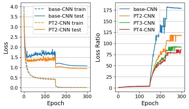
that under certain mild assumptions, instead of applying              Self training algorithms are used for representation learn-
each dihedral transformation to the input, one can compile            ing, by training a deep network to solve pretext tasks where
it into the CNN model’s weights by applying the inverse               labels can be produced directly from the data. Such tasks
transformation to the convolutional kernels. In order to ob-          include colorization [32, 16], placing image patches in the
tain intuition about the inductive bias of the model’s training       right place [22, 7], inpainting [23] and orientation predic-
algorithm in complex realistic frameworks, we analyze the             tion [10]. Typically, self-supervision is used in unsuper-
model’s inductive bias using a simplified framework.                  vised learning [8], to impose some structure on the data, or
    In Section 5 we describe our empirical results. We first          in semi-supervised learning [31, 12]. Our work is motivated
introduce a novel invariance score (IS), designed to mea-             by RotNet, an orientation prediction method suggested by
sure the model’s kernel invariance under a given group of             [10]. It differs from [31, 12], as we allocate a specific clas-
transformations. IS effectively measures the inductive bias           sification head for each input transformation rather than pre-
imposed on the model’s weights by the training algorithm.             dicting the self-supervised label with a separate head.
To achieve a fair comparison, we compare a regular CNN
                                                                      Equivariant CNNs. Many computer vision algorithms are
model traditionally trained, to the same model trained like
                                                                      designed to exhibit some form of invariance to a transfor-
a TransNet model as follows: heads are added to the base
                                                                      mation of the input, including geometric transformations
model, it is trained as a TransNet model, and then the extra
                                                                      [20], transformations of time [28], or changes in pose and
heads are pruned. We then show that training as TransNet
                                                                      illumination [24]. Equivariance is a more relaxed property,
improves test accuracy as compared to the base model. This
                                                                      exploited for example by CNN models when translation is
improvement was achieved while keeping the optimized
                                                                      concerned. Work on CNN models that enforces strict equiv-
hyper-parameters of the base CNN model, suggesting that
                                                                      ariance includes [26, 9, 1, 21, 2, 5]. Like these methods, our
further improvement by fine tuning may be possible. We
                                                                      method seeks to achieve invariance by employing weight
demonstrate the increased invariance of the model’s kernels
                                                                      sharing of the convolution layers between multiple heads.
when trained with TransNet.
                                                                      But unlike these methods, the invariance constraint is soft.
Our Contribution                                                      Soft equivariance is also seen in works like [6], which em-
                                                                      ploys a convolutional layer that simultaneously feeds ro-
   • Introduce TransNet - a model inspired by self-                   tated and flipped versions of the original image to a CNN
     supervision for supervised learning that imposes par-            model, or [30] that appends rotation and reflection versions
     tial invariance to a group of transformations.                   of each convolutional kernel.
   • Introduce an invariance score (IS) for CNN convolu-
     tional kernels.                                                  3. TransNet
   • Theoretical investigation of the inductive bias implied          Notations and definitions Let X = {(xi , yi )}ni=1 denote
     by the TransNet training algorithm.                              the training data, where xi ∈ Rd denotes the i-th data point
   • Demonstrate empirically how both the full and pruned             and yi ∈ [K] its corresponding label. Let D denote the
     versions of TransNet improve accuracy.                           data distribution from which the samples are drawn. Let H
                                                                      denote the set of hypotheses, where hθ ∈ H is defined by its
2. Related Work                                                       parameters θ (often we use h = hθ to simplify notations).
                                                                      Let `(h, x, y) denote the loss of hypothesis h when given
                                                                      sample (x, y). The overall loss is:
Overfit. A fundamental and long-standing issue in machine
learning, overfit occurs when a learning algorithm mini-                            L(h, X) = E(x,y)∼D [`(h, x, y)]              (1)
mizes the train loss, but generalizes poorly to the unseen
test set. Many methods were developed to mitigate this                Our objective is to find the optimal hypothesis:
problem, including early stopping - when training is halted
as soon as the loss over a validation set starts to increase,                            h∗ := arg min L(h, X)                   (2)
                                                                                                  h∈H
and regularization - when a penalty term is added to the
optimization loss. Other related ideas, which achieve sim-               For simplicity, whenever the underlying distribution of a
ilar goals, include dropout [27], batch normalization [14],           random variable isn’t explicitly defined we use the uniform
transfer learning [25, 29], and data augmentation [3, 33].                                               P|A|
                                                                      distribution, e.g. Ea∈A [a] = 1/|A| i=1 a.
Self-Supervised Learning. A family of learning algo-
                                                                      3.1. Model architecture
rithms that train a model using self generated labels (e.g.
the orientation of an image), in order to exploit unlabeled              The TransNet architecture is defined by a set of input
data as well as extract more information from labeled data.           transformations T = {tj }m
                                                                                               j=1 , where each transformation

                                                                  2
t ∈ T operates on the inputs (t : Rd → Rd ) and is associ- Algorithm 1: Training the TransNet model
ated with a corresponding model’s head. Thus each trans- input : TransNet model hT , batch size b,
formation operates on datapoint x as t(x), and the trans- maximum iterations num M AX IT ER
formed data-set is defined as: output: trained TransNet model
t(X) := {(t(xi ), yi )}ni=1 (3) 1 for i = 1 . . . M AX IT ER do
iid
2 sample a batch B = {(xk , yk )}bk=1 ∼ Db
Given an existing NN model h, henceforth called the 3 forward:
base model, we can split it to two components: all the lay- 4 for t ∈ T do
Pb
ers except for the last one denoted f , and the last layer g as- 5 L(ht , B) = 1b k=1 `(ht , t(xk ), yk )
sumed to be a fully-connected layer. Thus h = g ◦ f . Next, 6 end
we enhance model h by replacing g with |T| = m heads, 1
P
7 LT (hT , B) = m t∈T L(ht , B)
where each head is an independent fully connected layer gt 8 backward (SGD):
associated with a specific transformation t ∈ T. Formally, 9 update the model’s weights by differentiating
each head is defined by ht = gt ◦ f , and it operates on the the sampled loss LT (hT , B)
corresponding transformed input as ht (t(x)). 10 end
The full model, with its m heads, is denoted by hT :=
{ht }t∈T , and operates on the input as follows:
hT (x) := Et∈T [ht (t(x))] 3.3. Transformations
The corresponding loss of the full model is defined as:
Which transformations should we use? Given a specific
LT (hT , X) := Et∈T [L(ht , t(X))] (4) data-set, we distinguish between transformations that occur
naturally in the data-set versus such transformations that
Note that the resulting model (see Fig. 1) essentially rep- do not. For example, horizontal flip can naturally occur
resents m models, which share via f all the weights up to in the CIFAR-10 data-set, but not in the MNIST data-set.
the last fully-connected layer. Each of these models can be TransNet can only benefit from transformations that do not
used separately, as we do later on. occur naturally in the target data-set, in order for each head
to learn a well defined and non-overlapping classification
3.2. Training algorithm
task. Transformations that occur naturally in the data-set
Our method uses SGD with a few modifications to min- are often used for data augmentation, as by definition they
imize the transformation loss (4), as detailed in Alg. 1. Re- do not change the data domain.
lying on the fact that each batch is sampled i.i.d. from D,
we can prove (see Lemma 1) the desirable property that
the sampled loss LT (hT , B) is an unbiased estimator for Dihedral group D4 . As mentioned earlier, the TransNet
the transformation loss LT (hT , X). This justifies the use model is defined by a set of input transformations T. We
of Alg. 1 to optimize the transformation loss. constrain T to be a subset of the dihedral group D4 , which
includes reflections and rotations by multiplications of 90◦ .
Lemma 1. Given batch B, the sampled transformation loss We denote a horizontal reflection by m and a counter-
LT (hT , B) is an unbiased estimator for the transformation clockwise 90◦ rotation by r. Using these two elements we
loss LT (hT , X). can express all the D4 group elements as {ri , m ◦ ri | i ∈
0, 1, 2, 3}. These transformations were chosen because, as
Proof. mentioned in [10], their application is relatively efficient
and does not leave artifacts in the image (unlike scaling or
EB∼Db [LT (hT , B)] change of aspect ratio).
= EB∼Db [Et∈T [L(ht , t(B))]] Note that these transformations can be applied to any 3D
iid tensor while operating on the height and width dimensions,
= Et∈T [EB∼Db [L(ht , t(B))]] (B ∼ Db ) (5)
including an input image as well as the model’s kernels.
= Et∈T [L(ht , t(X))] When applying a transformation t to the model’s weights
= LT (hT , X) θ, denoted t(θ), the notation implies that t operates on the
model’s kernels separately, not affecting other layers such
as the fully-connected ones (see Fig. 2).
3sic model by appending additional heads:
k
Y
hT,θ = {gt ◦ linv ◦ ci }t∈T (7)
i=1
We denote the parameters of a fully-connected or a convo-
lutional layer by subscripts of w (weight) and b (bias), e.g.
g(x) = gw · x + gb .
4.1. Transformation compilation
Figure 2: The transformed input convolved with a kernel (upper Transformations in the dihedral D4 group satisfy another
path) equals to the transformation applied on the output of the in- important property, expressed by the following proposition:
put convolved with the inversely transformed kernel (lower path).
Proposition 1. Let hθ denote a CNN model where the last
3.4. Model variations convolutional layer is followed by an invariant layer under
Once trained, the full TransNet model can be viewed as the D4 group. Then any transformation t ∈ D4 applied to
an ensemble of m shared classifiers. Its time complexity the input image can be compiled into the model’s weights θ
is linear with the number of heads, almost equivalent to an as follows:
ensemble of the base CNN model, since the time needed
∀t ∈ D4 ∀x ∈ X : hθ (t(x)) = ht−1 (θ) (x) (8)
to apply each one of the D4 transformations to the input
is negligible as compared to the time needed for the model Proof. By induction on k we can show that:
to process the input. Differently, the space complexity is
almost equivalent to the space complexity of only one base k
Y k
Y
CNN model1 . ci ◦ t(x) = t ◦ t−1 (ci )(x) (9)
We note that one can prune each one of the model’s i=1 i=1
heads, thus leaving a smaller ensemble of up to m classi-
(see Fig. 2). Plugging (9) into (6), we get:
fiers. A useful reduction prunes all the model’s heads except
one, typically the one corresponding to the identity trans- k
Y
formation, which yields a regular CNN that is equivalent hθ (t(x)) = g ◦ linv ◦ ci ◦ t(x)
in terms of time and space complexity to the base architec- i=1
ture used to build the TransNet model. Having done so, we k
Y
can evaluate the effect of the TransNet architecture’s and = g ◦ linv ◦ t ◦ t−1 (ci )(x)
its training algorithm’s inductive bias solely on the training i=1
procedure, by comparing the pruned TransNet to the base k
Y
CNN model (see Section 5). = g ◦ linv ◦ t−1 (ci )(x) (linv ◦ t = linv )
i=1
4. Theoretical Analysis = ht−1 (θ) (x)
In this section we analyze theoretically the TransNet
model. We consider the following basic CNN architecture:
k Implication. The ResNet model [11] used in our exper-
Y
hθ = g ◦ linv ◦ ci (6) iments satisfies the pre-condition in the proposition stated
i=1 above, since it contains a GAP layer [19] after the last con-
volutional layer, and GAP is invariant under D4 .
where g denotes a fully-connected layer, linv denotes an
invariant layer under the D4 transformations group (e.g. a 4.2. Single vs. multiple headed model
global average pooling layer - GAP), and {ci }i∈[k] denote In order to acquire intuition regarding the inductive bias
convolutional layers2 . The TransNet model extends the ba- implied by training algorithm Alg. 1, we consider two cases,
1 Each additional head adds 102K (∼0.45%) and 513K (∼0.90%) extra a single and a double headed model, trained with the same
parameters to the basic ResNet18 model when training CIFAR-100 and training algorithm. A single headed model is a special case
ImageNet-200 respectively. of the full multi-headed model, where all the heads share
2 While each convolutional layer may be followed by ReLU and Batch
Normalization [14] layers, this doesn’t change the analysis so we obviate weights ht (t(x)) = h(t(x)) ∀t, and the loss in line 5 of
Pb
the extra notation. Alg. 1 becomes L(h, B) = 1b k=1 `(h, t(xk ), yk ).
4As it’s hard to analyze non-convex deep neural networks, head. Each gi outputs a vector of size 2. The data-set
we focus on a simplified framework and consider a con- X = {(x1 , y1 ), (x2 , y2 )} consists of 2 examples:
vex optimization problem where the loss function is convex
w.r.t. the model’s parameters θ. We also assume that the 1 1 1 0 0 0
model’s transformations in T form a group3 . x1 = 0 0 0 , y1 = 1, x2 = 0 0 0 , y2 = 2
0 0 0 1 1 1
Single Headed model Analysis. In this simplified case, we
can prove the following strict proposition: Note that x2 = t2 (x1 )4 .
Proposition 2. Let hθ denote a CNN model satisfying the Now, assume the model’s convolutional layer c is com-
pre-condition of Prop. 1, and T ⊂ D4 a transformations posed of 2 invariant kernels under T, and denote it by cinv .
group. Then the optimal transformation loss LT (see Eq. 4) Let i ∈ 1, 2, then:
is obtained by invariant model’s weights under the transfor-
hi (x2 ) = hi (t2 (x1 )) = gi ◦ GAP ◦ cinv ◦ t2 (x1 )
mations T. Formally: (10)
= gi ◦ GAP ◦ cinv (x1 ) = hi (x1 )
∃θ0 : (∀t ∈ T : θ0 = t(θ0 )) ∧ (θ0 ∈ arg min LT (θ, X))
θ In this case both heads predict the same output for both
inputs with different labels, thus:
Proof. To simplify the notations, henceforth we let θ de-
note the model hθ .
L(hi , ti (X)) > 0 =⇒ LT (hT,θ , X) > 0
LT (θ, X)
In contrast, by setting cw = (x1 , x2 ), cb = (0, 0), which
= Et∈T [L(θ, t(X))] isn’t invariant under T, as well as:
= Et∈T [E(x,y)∼D [`(θ, t(x), y)]]
1 0 0 0 1 0
= Et∈T [E(x,y)∼D [`(t−1 (θ), x, y)]] (by Prop. 1) g1,w = , g1,b = g2,w = , g2,b = ,
0 1 0 1 0 0
= E(x,y)∼D [Et∈T [`(t−1 (θ), x, y)]]
≥ E(x,y)∼D [`(Et∈T [t−1 (θ)], x, y)] (Jensen’s inequality) we obtain:
= E(x,y)∼D [`(θ̄, x, y)] (θ̄ := Et∈T [t(θ))], T = T−1 ) L(hi , ti (X)) = 0 =⇒ LT (hT,θ , X) = 0.
= L(θ̄, X)
We may conclude that the optimal model’s kernels aren’t
= Et∈T [L(t−1 (θ̄), X)] (θ̄ is invariant under T)
invariant under T, as opposed to the claim of Prop. 2.
= Et∈T [L(θ̄, t(X))] (by Prop. 1)
= LT (θ̄, X) Discussion. The intuition we derive from the analysis above
is that the training algorithm (Alg. 1) implies an invariant
Above we use the fact that θ̄ is invariant under T since T is inductive bias on the model’s kernels as proved in the sin-
a group and thus t0 T = T, hence: gle headed model, while not strictly enforcing invariance as
shown by the counter example of the double headed model.
t0 (θ̄) = t0 (Et∈T [t(θ)]) = Et∈T [t0 ◦t(θ)] = Et∈T [t(θ)] = θ̄
5. Experimental Results
Double headed model. In light of Prop. 2 we now present data-sets. For evaluation we used the 5 image classification
a counter example, which shows that Prop. 2 isn’t true for data-sets detailed in Table 1. These diverse data-sets allow
the general TransNet model. us to evaluate our method across different image resolutions
and number of predicted classes.
Example 1. Let T = {t1 = r0 , t2 = m ◦ r2 } ⊂ D4
denote the transformations group consisting of the iden- Implementation Details. We employed the ResNet18 [11]
tity and the vertical reflection transformations. Let hT,θ = architecture for all the data-sets except for ImageNet-200,
{hi = gi ◦ GAP ◦ c}2i=1 denote a double headed TransNet which was evaluated using the ResNet50 architecture (see
model, which comprises a single convolutional layer (1 Appendix A for more implementation details).
channel in and 2 channels out), followed by a GAP layer Notations.
and then 2 fully-connected layers {gi }2i=1 , one for each
4 This example may seem rather artificial, but in fact this isn’t such a
3T being a group is a technical constraint needed for the analysis, not rare case. E.g., the airplane and the ship classes, both found in the CIFAR-
required by the algorithm. 10 data-set, that share similar blue background.
5Name Classes Train/Test dim comparing the ”Tm-CNN” models with the ”base-CNN”
Samples model, see Table 3. Despite the fact that the full TransNet
CIFAR-10 [15] 10 50K/10K 32 model processes the (transformed) input m times more as
CIFAR-100 [15] 100 50K/10K 32 compared to the ”base-CNN” model, its architecture is not
ImageNette [13] 10 10K/4K 224 significantly larger than the base-CNN’s. The full TransNet
ImageWoof [13] 10 10K/4K 224 adds to the ”base-CNN” a negligible number of parame-
ImageNet-200 200 260K/10K 224 ters, in the form of its multiple heads1 . Clearly the full
TransNet model improves the accuracy as compared to the
Table 1: The data-sets used in our experiments. The dimension of ”base-CNN” model, and also as compared to the pruned
each example, a color image, is dim×dim×3 pixels. ImageNette TransNet model. Thus, if the additional runtime complexity
represents 10 easy to classify classes from ImageNet [4], while Im-
during test is not an issue, it is beneficial to employ the full
ageWoof represents 10 hard to classify classes of dog breeds from
ImageNet. ImageNet-200 represents 200 classes from ImageNet
TransNet model during test time. In fact, one can process
(same classes as in [17]) of full size images. the input image once, and then choose whether to continue
processing it with the other heads to improve the prediction,
all this while keeping roughly the same space complexity.
• ”base CNN” - a regular convolutional neural network,
identical to the TransNet model with only the head cor- Ensembles: models with similar time complexity, dif-
responding to the identity transformation. ferent space complexity. Here we evaluate ensembles of
• ”PTm-CNN” - a pruned TransNet model trained with pruned TransNet models, and compare them to a single full
m heads, where a single head is left and used for pre- TransNet model that can be seen as a space-efficient ensem-
diction5 . It has the same space and time complexity as ble: full TransNet generates m predictions with only 1/m
the base CNN. parameters, where m is the number of TransNet heads. Re-
sults are shown in Fig. 3. Clearly an ensemble of pruned
• ”Tm-CNN” - a full TransNet model trained with m
TransNet models is superior to an ensemble of base CNN
heads, where all are used for prediction. It has roughly
models, suggesting that the accuracy gain achieved by the
the same space complexity1 and m times the time com-
pruned TransNet model doesn’t overlap with the accuracy
plexity as compared to the base CNN.
gain achieved by using an ensemble of classifiers. Fur-
To denote an ensemble of the models above, we add a suffix thermore, we observe that the full TransNet model exhibits
of a number in parentheses, e.g. T2-CNN (3) is an ensemble competitive accuracy results, with 2 and 3 heads, as com-
of 3 T2-CNN models. pared to an ensemble of 2 or 3 base CNN models respec-
tively. This is achieved while utilizing 1/2 and 1/3 as
5.1. Models accuracy, comparative results many parameters respectively.
We now compare the accuracy of the ”base-CNN”,
”PTm-CNN” and ”Tm-CNN” models, where m = 2, 3, 4
denotes the number of heads of the TransNet model, and
their ensembles, across all the data-sets listed in Table 1.
Models with the same space and time complexity. First,
we evaluate the pruned TransNet model by comparing the
”PTm-CNN” models with the ”base-CNN” model, see Ta-
ble 2. Essentially, we evaluate the effect of using the
TransNet model only for training, as the final ”PTm-CNN”
models are identical to the ”base-CNN” model regardless
of m. We can clearly see the inductive bias implied by
the training procedure. We also see that TransNet training
improves the accuracy of the final ”base-CNN” classifier
across all the evaluated data-sets.
Models with similar space complexity, different time Figure 3: Model accuracy as a function of the number of instances
complexity. Next, we evaluate the full TransNet model by (X-axis) processed during prediction. Each instance requires a
complete run from input to output. An ensemble includes: m in-
5 In our experiments we chose the head associated with the identity (r 0 )
dependent base CNN classifiers for ”CNN”; m pruned TransNet
transformation when evaluating a pruned TransNet. Note, however, that we
trained with 2 heads for ”PT2-CNN”; and one TransNet model
could have chosen the best head in terms of accuracy, as it follows from
Prop. 1 that its transformation can be compiled into the model’s weights. with m heads, where m is the ensemble size, for ”Tm-CNN”.
6MODEL CIFAR-10 CIFAR-100 ImageNette ImageWoof ImageNet-200
base-CNN 95.57 ± 0.08 76.56 ± 0.16 92.97 ± 0.16 87.27 ± 0.15 84.39 ± 0.07
PT2-CNN 95.99 ± 0.07 79.33 ± 0.15 93.84 ± 0.14 88.09 ± 0.30 85.17 ± 0.10
PT3-CNN 95.87 ± 0.04 79.08 ± 0.06 94.15 ± 0.16 87.79 ± 0.11 84.97 ± 0.95
PT4-CNN 95.73 ± 0.05 77.98 ± 0.17 93.94 ± 0.06 85.81 ± 0.79 84.02 ± 0.71
Table 2: Accuracy of models with the same space and time complexity, comparing the Base CNN with pruned TransNet models ”PTm-
CNN”, where m = 2, 3, 4 denotes the number of heads in training. Mean and standard error for 3 repetitions are shown.
MODEL CIFAR-10 CIFAR-100 ImageNette ImageWoof ImageNet-200
base-CNN 95.57 ± 0.08 76.56 ± 0.16 92.97 ± 0.16 87.27 ± 0.15 84.39 ± 0.07
T2-CNN 96.22 ± 0.10 80.35 ± 0.06 94.02 ± 0.13 88.36 ± 0.33 85.47 ± 0.14
T3-CNN 96.33 ± 0.06 80.92 ± 0.08 94.39 ± 0.07 88.79 ± 0.25 85.68 ± 0.20
T4-CNN 96.17 ± 0.01 79.94 ± 0.16 94.67 ± 0.06 87.05 ± 0.75 85.54 ± 0.11
Table 3: Accuracy of models with similar space complexity and different time complexity, comparing the Base CNN with full TransNet
models. With m denoting the number of heads, chosen to be 2,3 or 4, the prediction time complexity of the respective TransNet model
”Tm-CNN” is m times larger than the base CNN. Mean and standard error for 3 repetitions are shown.
Accuracy vs. generalization. In Fig. 3 we can see that 2 TransNet models exhibit better generalization when com-
heads improve the model’s performance across all data-sets, pared to the base CNN model. Furthermore, the generaliza-
3 heads improve it on most of the data-sets, and 4 heads ac- tion improvement increases with the number of TransNet
tually reduce performance on most data-sets. We hypothe- model heads, which are only used for training and then
size that too many heads impose too strict an inductive bias pruned. The observed narrowing of the generalization gap
on the model’s kernels. Thus, although generalization is im- occurs because, although the TransNet model slightly in-
proved, test accuracy is reduced due to insufficient variance. creases the training loss, it more significantly decreases the
Further analysis is presented in the next section. test loss as compared to the base CNN.
5.2. Generalization
We’ve seen in Section 5.1 that the TransNet model,
whether full or pruned, achieves better test accuracy as com-
pared to the base CNN model. This occurs despite the fact
that the transformation loss LT (hT , X) minimized by the
TransNet model is more demanding than the loss L(h, X)
minimized by the base CNN, and appears harder to opti-
mize. This conjecture is justified by the following Lemma:
Lemma 2. Let hT denote a TransNet model that obtains
transformation loss of a := LT (hT , X). Then there exists a
reduction from hT to the base CNN model h that obtains a
loss of at most a, i.e. L(h, X) ≤ a. Figure 4: CIFAR-100 results. Left panel: learning curve of the
Proof. a = LT (hT , X) = Et∈T [L(hθt , t(X))], so there Base CNN model (”base-CNN”) and a pruned TransNet model
must be a transformation t ∈ T s.t. L(hθt , t(X)) ≤ a. (”PT2-CNN”). Right panel: generalization score, test-train loss
ratio, measured for the base-CNN model and various pruned
Now, one can compile the transformation t into hθt (see
TransNet models with a different number of heads.
Prop. 1) and get a base CNN: h̃ = ht−1 (θt ) which obtains
L(h̃, X) = L(ht−1 (θt ) , t(X)) = L(hθt , t(X)) ≤ a.
We note that better generalization does not necessarily
Why is it, then, that the TransNet model achieves overall imply a better model. The ”PT4-CNN” model generalizes
better accuracy than the base CNN? The answer lies in its better than any other model (see right panel of Fig. 4), but
ability to achieve a better generalization. its test accuracy is lower as seen in Table 2.
In order to measure the generalization capability of a
5.3. Kernel invariance
model w.r.t. a data-set, we use the ratio between the test-
set and train-set loss, where a lower ratio indicates better What characterizes the beneficial inductive bias implied
generalization. As illustrated in Fig. 4, clearly the pruned by the TransNet model and its training algorithm Alg. 1?.
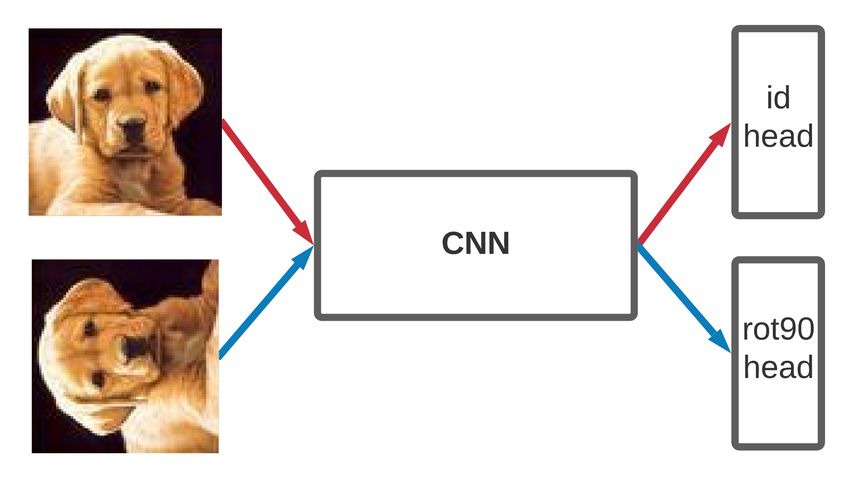
7To answer this question, we investigate the emerging invari- TransNet models exhibits much higher invariance level as
ance of kernels in the convolutional layers of the learned compared to the base CNN. This phenomenon is robust to
network, w.r.t. the TransNet transformations set T. the metric used in the IS definition, with similar results
We start by introducing the ”Invariance Score” (IS), when using ”Pearson Correlation” or ”Cosine Similarity”.
which measures how invariant a 3D tensor is w.r.t. a trans- The increased invariance in the last convolutional layer is
formations group. Specifically, given a convolutional kernel monotonically increasing with the number of heads in the
denoted by w (3D tensor) and a set of transformations group TransNet model, which is consistent with the generalization
T, the IS score is defined as follows: capability of these models (see Fig 4).
IS(w, T) := min kw − uk (11)
u∈IN VT
where IN VT is the set of invariant kernels (same shape as
w) under T, i.e. IN VT := {u : u = t(u) ∀t ∈ T}.
Lemma 3. arg minu∈IN VT kw − uk = Et∈T [t(w)]
Proof. Let u be an invariant tensor under T. Define
2
f (u) := kw − uk . Note that arg minu∈IN VT kw − uk =
arg minu∈IN VT f (u).
2
f (u) = kw − uk
2 Figure 5: CIFAR-100 results, plotting the distribution of the IS
= Et∈T [kw − t(u)k ] (u is invariant under T)
2 scores (mean and std) for the kernels in each layer of the different
= Et∈T [ t−1 (w) − u ] models. Invariance is measured w.r.t. the group of 90◦ rotations.
2
= Et∈T [kt(w) − uk ] (T = T−1 )
size(w)
X
= Et∈T [ (t(w)i − ui )2 ]
i=1
Where index i runs over all the tensors’ elements. Finally,
we differentiate f to obtain its minimum:
∂f
= Et∈T [−2(t(w)i − ui )] = 0
∂ui
=⇒ ui = Et∈T [[t(w)i ] =⇒ u = Et∈T [t(w)]
Lemma 3 gives a closed-form expression for the IS gauge:
IS(w, T) = kw − Et∈T [t(w)]k (12)
Figure 6: CIFAR-100 results, plotting the full distribution of the
Equipped with this gauge, we can inspect the invari- IS scores for the kernels in the last (17-th) layer of the different
ance level of the model’s kernels w.r.t. a transformations models. Invariance is measured w.r.t. the group of 90◦ rotations.
group. Note that this measure allows us to compare the full
The generalization improvement achieved by the
TransNet model with the base CNN model, as both share
TransNet model, as reported in Section 5.2, may be ex-
the same convolution layers. Since the transformations of
plained by this increased level of invariance, as highly in-
the TransNet model don’t necessarily form a group, we use
variant kernels have fewer degrees of freedom, and should
the minimal group containing these transformations - the
therefore be less prone to overfit.
group of all rotations {ri }4i=1 .
In Fig. 5 we can see that the full TransNet model ”T2- 5.4. Ablation Study
CNN” and the base CNN model demonstrate similar in-
variance level in all the convolutional layers but the last Our method consists of 2 main components - the
one. In Fig. 6, where the distribution of the IS score over TransNet architecture as well as the training algorithm
the last layer of 4 different models is fully shown, we can Alg. 1. To evaluate the accuracy gain of each component
more clearly see that the last convolutional layer of full we consider two variations:
8MODEL CIFAR-10 CIFAR-100 ImageNette ImageWoof ImageNet-200
base-CNN 95.57 ± 0.08 76.56 ± 0.16 92.97 ± 0.16 87.27 ± 0.15 84.39 ± 0.07
Alg. only 93.85 ± 0.63 76.64 ± 0.69 92.60 ± 0.07 87.64 ± 0.30 80.58 ± 0.08
Arch. only 95.68 ± 0.05 76.98 ± 0.13 93.49 ± 0.03 87.40 ± 0.74 84.47 ± 0.13
PT2-CNN 95.99 ± 0.07 79.33 ± 0.15 93.84 ± 0.14 88.09 ± 0.30 85.17 ± 0.10
Table 4: Accuracy of the ablation study models with the same space and time complexity, these 4 models enable us to evaluate the effect
of the TransNet architecture as well as the TransNet algorithm separately. Mean and standard error for 3 repetitions are shown.
• Architecture only: in this method we train the multi- Acknowledgements
headed architecture (2 in this case) by feeding each
head the same un-transformed batch (equivalent to a This work was supported in part by a grant from the Is-
TransNet model with the multi-set of {id, id} transfor- rael Science Foundation (ISF) and by the Gatsby Charitable
mations). Prediction is retrieved from a single head Foundations.
(similar to PT2-CNN).
References
• Algorithm only: in this method we train the base (one [1] Christopher Clark and Amos Storkey. Training deep convo-
headed) model by the same algorithm Alg. 1. (This lutional neural networks to play go. In International confer-
model was also considered in the theoretical part 4.2, ence on machine learning, pages 1766–1774, 2015. 2
termed single headed model.) [2] Taco Cohen and Max Welling. Group equivariant convo-
lutional networks. In International conference on machine
learning, pages 2990–2999, 2016. 2
We compare the two methods above to the ”base-CNN”
[3] Ekin D Cubuk, Barret Zoph, Dandelion Mane, Vijay Vasude-
regular model and the complete model ”PT2-CNN”, see
van, and Quoc V Le. Autoaugment: Learning augmentation
Table 4. We can see that using only one of the compo-
strategies from data. In Proceedings of the IEEE conference
nents doesn’t yield any significant accuracy gain. This sug- on computer vision and pattern recognition, pages 113–123,
gest that the complete model benefits from both compo- 2019. 2
nents working together: the training algorithm increases the [4] Jia Deng, Wei Dong, Richard Socher, Li-Jia Li, Kai Li,
model kernel’s invariance on the one hand, while the multi- and Li Fei-Fei. Imagenet: A large-scale hierarchical image
heads architecture encourage the model to capture meaning- database. In 2009 IEEE conference on computer vision and
ful orientation information on the other hand. pattern recognition, pages 248–255. Ieee, 2009. 6
[5] Sander Dieleman, Jeffrey De Fauw, and Koray Kavukcuoglu.
Exploiting cyclic symmetry in convolutional neural net-
6. Summary works. arXiv preprint arXiv:1602.02660, 2016. 2
[6] Sander Dieleman, Kyle W Willett, and Joni Dambre.
We introduced a model inspired by self-supervision, Rotation-invariant convolutional neural networks for galaxy
which includes a base CNN model attached to multiple morphology prediction. Monthly notices of the royal astro-
heads, each corresponding to a different transformation nomical society, 450(2):1441–1459, 2015. 2
from a fixed set of transformations. The self-supervised as- [7] Carl Doersch, Abhinav Gupta, and Alexei A Efros. Unsuper-
pect of the model is crucial, as the chosen transformations vised visual representation learning by context prediction. In
must not occur naturally in the data. When the model is Proceedings of the IEEE international conference on com-
pruned back to match the base CNN, it achieves better test puter vision, pages 1422–1430, 2015. 2
accuracy and improved generalization, which is attributed [8] Alexey Dosovitskiy, Philipp Fischer, Jost Tobias Springen-
to the increased invariance of the model’s kernels in the last berg, Martin Riedmiller, and Thomas Brox. Discriminative
layer. We observed that excess invariance, while improving unsupervised feature learning with exemplar convolutional
generalization, eventually curtails the test accuracy. neural networks. IEEE transactions on pattern analysis and
machine intelligence, 38(9):1734–1747, 2015. 2
We evaluated our model on various image data-sets, ob- [9] Robert Gens and Pedro M Domingos. Deep symmetry net-
serving that each data-set achieves its own optimal ker- works. In Advances in neural information processing sys-
nel’s invariance level, i.e. there’s no optimal number of tems, pages 2537–2545, 2014. 2
heads for all data-sets. Finally, we introduced an invari- [10] Spyros Gidaris, Praveer Singh, and Nikos Komodakis. Un-
ance score gauge (IS), which measures the level of invari- supervised representation learning by predicting image rota-
ance achieved by the model’s kernels. IS may be leveraged tions. arXiv preprint arXiv:1803.07728, 2018. 2, 3
to determine the optimal invariance level, as well as poten- [11] Kaiming He, Xiangyu Zhang, Shaoqing Ren, and Jian Sun.
tially function as an independent regularization term. Deep residual learning for image recognition. In Proceed-
9ings of the IEEE conference on computer vision and pattern [29] Karl Weiss, Taghi M Khoshgoftaar, and DingDing Wang. A
recognition, pages 770–778, 2016. 4, 5, 10 survey of transfer learning. Journal of Big data, 3(1):9, 2016.
[12] Dan Hendrycks, Mantas Mazeika, Saurav Kadavath, and 2
Dawn Song. Using self-supervised learning can improve [30] Fa Wu, Peijun Hu, and Dexing Kong. Flip-rotate-
model robustness and uncertainty. In Advances in Neural pooling convolution and split dropout on convolution neu-
Information Processing Systems, pages 15663–15674, 2019. ral networks for image classification. arXiv preprint
2 arXiv:1507.08754, 2015. 2
[13] Jeremy Howard. Imagewang. 6 [31] Xiaohua Zhai, Avital Oliver, Alexander Kolesnikov, and Lu-
[14] Sergey Ioffe and Christian Szegedy. Batch normalization: cas Beyer. S4l: Self-supervised semi-supervised learning. In
Accelerating deep network training by reducing internal co- Proceedings of the IEEE international conference on com-
variate shift. arXiv preprint arXiv:1502.03167, 2015. 2, 4 puter vision, pages 1476–1485, 2019. 2
[15] Alex Krizhevsky, Geoffrey Hinton, et al. Learning multiple [32] Richard Zhang, Phillip Isola, and Alexei A Efros. Colorful
layers of features from tiny images. 2009. 6 image colorization. In European conference on computer
[16] Gustav Larsson, Michael Maire, and Gregory vision, pages 649–666. Springer, 2016. 2
Shakhnarovich. Learning representations for automatic [33] Zhun Zhong, Liang Zheng, Guoliang Kang, Shaozi Li, and
colorization. In European conference on computer vision, Yi Yang. Random erasing data augmentation. In AAAI, pages
pages 577–593. Springer, 2016. 2 13001–13008, 2020. 2
[17] Ya Le and Xuan Yang. Tiny imagenet visual recognition
challenge. CS 231N, 7, 2015. 6 Appendix
[18] Chen-Yu Lee, Saining Xie, Patrick Gallagher, Zhengyou
Zhang, and Zhuowen Tu. Deeply-supervised nets. In Ar- A. Implementation details
tificial intelligence and statistics, pages 562–570, 2015. 10
We employed the ResNet [11] architecture, specifically
[19] Min Lin, Qiang Chen, and Shuicheng Yan. Network in net-
work. arXiv preprint arXiv:1312.4400, 2013. 4 the ResNet18 architecture for all the data-sets except for the
[20] Joseph L Mundy, Andrew Zisserman, et al. Geometric in- ImageNet-200 which was evaluated using the ResNet50 ar-
variance in computer vision, volume 92. MIT press Cam- chitecture. It’s important to notice that we haven’t changed
bridge, MA, 1992. 2 the hyper-parameters used by the regular CNN architecture
[21] Jiquan Ngiam, Zhenghao Chen, Daniel Chia, Pang W Koh, which TransNet is based on. This may strengthen the results
Quoc V Le, and Andrew Y Ng. Tiled convolutional neu- as one may fine tune these hyper-parameters to suit best the
ral networks. In Advances in neural information processing TransNet model.
systems, pages 1279–1287, 2010. 2 We used a weight decay of 0.0001 and momentum of
[22] Mehdi Noroozi and Paolo Favaro. Unsupervised learning 0.9. The model was trained with a batch size of 64 for all
of visual representations by solving jigsaw puzzles (2016). the data-sets except for ImageNet-200 where we increased
arXiv preprint arXiv:1603.09246. 2 the batch size to 128. We trained the model for 300 epochs,
[23] Deepak Pathak, Philipp Krahenbuhl, Jeff Donahue, Trevor starting with a learning rate of 0.1, divided by 10 at the 150
Darrell, and Alexei A. Efros. Context encoders: Feature and 225 epochs, except for the ImageNet-200 model which
learning by inpainting, 2016. 2
was trained for 120 epochs, starting with a learning rate of
[24] Pascal Paysan, Reinhard Knothe, Brian Amberg, Sami
0.1, divided by 10 at the 40 and 80 epochs. We normalized
Romdhani, and Thomas Vetter. A 3d face model for pose
and illumination invariant face recognition. In 2009 Sixth
the images as usual by subtracting the image’s mean and
IEEE International Conference on Advanced Video and Sig- dividing by the image’s standard deviation (color-wise).
nal Based Surveillance, pages 296–301. Ieee, 2009. 2 We employed a mild data augmentation scheme - hori-
[25] Ling Shao, Fan Zhu, and Xuelong Li. Transfer learning for zontal flip with probability of 0.5. For the CIFAR data-sets
visual categorization: A survey. IEEE transactions on neural we padded each dimension by 4 pixels and cropped ran-
networks and learning systems, 26(5):1019–1034, 2014. 2 domly (uniform) a 32×32 patch from the enlarged image
[26] Laurent Sifre and Stéphane Mallat. Rotation, scaling and [18] while for the ImageNet family data-sets we cropped
deformation invariant scattering for texture discrimination. randomly (uniform) a 224×224 patch from the original im-
In Proceedings of the IEEE conference on computer vision age.
and pattern recognition, pages 1233–1240, 2013. 2 In test time, we took the original image for the CIFAR
[27] Nitish Srivastava, Geoffrey Hinton, Alex Krizhevsky, Ilya data-sets and a center crop for the ImageNet family data-
Sutskever, and Ruslan Salakhutdinov. Dropout: a simple way sets. The prediction of each model is the mean of the
to prevent neural networks from overfitting. The journal of
model’s output on the original image and a horizontally
machine learning research, 15(1):1929–1958, 2014. 2
flipped version of it. Note that a horizontal flip occurs nat-
[28] Pavan Turaga and Rama Chellappa. Locally time-invariant
urally in every data-set we use for evaluation and therefore
models of human activities using trajectories on the grass-
mannian. In 2009 IEEE Conference on Computer Vision and isn’t associated with any of the TransNet model’s heads that
Pattern Recognition, pages 2435–2441. IEEE, 2009. 2 we evaluate.
10You can also read