Error indicators for controlling automatic grid refinement in ISIS-CFD Zaib Ali - Master of Science Thesis Ecole Centrale de Nantes, France ...
←
→
Page content transcription
If your browser does not render page correctly, please read the page content below
Error indicators for controlling automatic grid
           refinement in ISIS-CFD

                   Zaib Ali

           Master of Science Thesis
        Ecole Centrale de Nantes, France

         Supervisor: Dr. Jeroen Wackers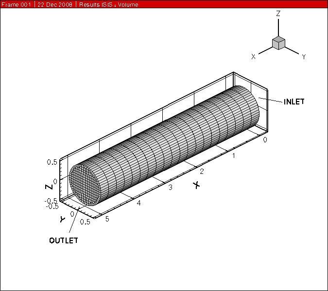
Abstract
This master’s thesis work is a part of the effort to build various error indicators or
refinement criteria for the adaptive grid refinement part of the ISIS-CFD flow solver. The
purpose is to develop such refinement criteria which respond to the needs of the flow
solver users and are general and flexible. Three types of refinement criteria are tested for
various flow and refinement conditions. We focus here on the capturing of vortices to
observe the performance of refinement criteria. Two test cases are used for this purpose.
The work is done on the initial stages and more in-depth analysis of the refinement
criteria is proposed in order to use them efficiently.

                                             2
Acknowledgements
I would like to express the deepest appreciation to Dr. Jeroen Wackers, my thesis
supervisor, who has the attitude and the substance of a genius: he continually and
convincingly conveyed a spirit of adventure in regard to research during the whole
period. Without his guidance and persistent help this dissertation would not have been
possible.
I thank Dr. Michel Visonneau, the head of CFD research group at Ecole Centrale de
Nantes, who gave me the opportunity to work with his research group. His constant
support and encouragement kept me motivated throughout the project.
This work would never have been accomplished without the help of Dr. Patrick Queutey and
Dr. Emmanuel Guilmineau. They spent a lot of time guiding me and were always available
to help me. I am grateful for their countless help, support, discussion and guidance.
Last but not the least; I would like to express my gratitude to my loving parents, brother and
sister for supporting and encouraging me throughout my life.
3Table of contents
1. Introduction……………………………………………………………….……………7
2. Adaptive grid refinement in ISIS-CFD………………………………………………...8
2.1 The flow solver ISIS-CFD………………………………………………………… 8
2.2 Mesh adaptation…………………………………………………………………….8
2.3 Local mesh adaptation in ISIS-CFD................................................................…....10
2.3.1 Organization and data structure………………………………………………10
2.3.1.1 Relationship between the cells………………………………………11
2.3.1.2 Activity of the cells …………………………………………………13
2.3.2 Grid refinement and coarsening………………………………………………13
2.3.3 Refinement procedure………………………………………………………..15
3. Error indicators for adaptive mesh refinement……………………………………….18
3.1 Refinement Criteria……………………………………………………………….19
3.2 A simple vortex flow problem…………………………………………………… 20
4. KVLCC2 Test Case………………………………………………………………….. 29
4.1 Geometry and conditions………………………………………………………….29
4.2 Computations ……………………………………………………………………..30
4.3 Results …………………………………………………………………………….31
4.3.1. Effect of the boundary layer refinement……………………………………..31
4.3.2 Computations without boundary layer refinement…………………………. .38
4.3.3 Computations with EASM turbulence model………………………………...40
5. The NACA 16020 at incidence………………………………………………………..42
5.1 Mesh and numerical conditions ………………………………………………….42
5.2 Computations……………………………………………………………………..43
5.3 Results…………………………………………………………………………….45
Conclusions …………………………………………………………...............................51
References………………………………………………………………………………. 52
4List of figures
Figure 2.1: Mother-daughter-sister connections between cells of the same generation…12
Figure 2.2: Mother-sister-daughter connections of cells between several generations.....12
Figure 2.3: Isotropic refinement of a hexahedron…………………………………….....14
Figure 2.4: Refinements of a quadrangle……………………………………………….. 14
Figure 2.5: Hanging node………………………………………………………………. 14
Figure 2.6: Adaptive procedure……………………………………………………….....16
Figure 3.1: Cylinder geometry and computational domain……………………………...21
Figure 3.2: The coarse 4.4K cell Uniform grid cross section……………………………22
Figure 3.3: The refined 2.1M cells uniform grid………………………………………...22
Figure 3.4: Pressure integral plot for velocity gradient criteria at x = 4.5……………….25
Figure 3.5: Pressure integral plot for pressure gradient criteria at x = 4.5………………25
Figure 3.6: Pressure integral plot for vorticity criteria at x = 4.5………………………..26
Figure 3.7: Pressure integral plot for three criteria at x = 4.5 for maximum threshold….26
Figure 3.8: Effect of number of generations on the refinement………………………....27
Figure 3.9: Pressure contours for velocity gradient criteria at maximum threshold…….28
Figure 4.1: KVLCC2 scale model……………………………………………………….29
Figure 4.2: Velocity gradient criterion for 1st threshold and 3 generations. ……………32
Figure 4.3: Velocity gradient criterion for 2nd threshold and 3 generations. …………... 32
Figure 4.4: Velocity gradient criterion for 3rd threshold and 2 generations. …………....33
Figure 4.5: Vorticity criterion for 1st threshold and 3 generations. ……………………. 34
Figure 4.6: Vorticity criterion for 2nd threshold and 3 generations. …………………….34
Figure 4.7: Vorticity criterion for 3rd threshold and 2 generations. …………………….35
Figure 4.8: Pressure gradient criterion for 1st threshold and 3 generations. ……………36
Figure 4.9: Pressure gradient criterion for 2nd threshold and 3 generations……………36
Figure 4.10: Pressure gradient criterion for 3rd threshold and 2 generations. …………..37
Figure 4.11: Velocity gradient criterion………………………………………………....38
Figure 4.12: Vorticity criterion. Propeller plane mesh and axial velocity contour. …….39
Figure 4.13: Pressure gradient criterion. ………………………………………………...39
Figure 4.14: KVLCC2 tanker, cuts in the propeller plane. ……………………………...41
Figure 5.1: NACA 16020 Computational domain.............................................................43
Figure 5.2: Surface mesh...................................................................................................43
Figure 5.3: Original (0.5M cells) mesh and pressure contour at X/Cmax = 0.6…………..46
Figure 5.4: Uniformly refined (4M cells) mesh and pressure contour at X/Cmax = 0.6 ....46
Figure 5.5: Velocity gradient criterion, minimum threshold and 3 generations………....46
Figure 5.6: Vorticity criterion, minimum threshold and 3 generations………………….47
Figure 5.7: Pressure Gradient criterion, maximum threshold and 2 generations…….….47
Figure 5.8: Pressure Gradient criterion, minimum threshold and 2 generations………...47
Figure 5.9: Velocity gradient criterion, without boundary layer refinement. …………...48
Figure 5.10: Vorticity criterion, without boundary layer refinement …………………...48
Figure 5.11: Velocity gradient criterion, without boundary layer refinement ………......48
Figure 5.12: Axial velocity profile at X/Cmax = 0.6 ………………………………….….49
Figure 5.13: Tangential velocity profile at X/Cmax = 0.6 ……………………………..…49
Figure 5.14: Pressure (KPa) profile at X/Cmax = 0.6 ………………………………….....50
5List of tables
Table 3.1: Uniform grids data……………………………………………………..……21
Table 3.2: Automatic grid refinement data for velocity gradient criterion………..……23
Table 3.3: Automatic grid refinement data for vorticity criterion…………………..…. 23
Table 3.4: Automatic grid refinement data for pressure gradient criterion………..……24
Table 4.1: Automatic grid refinement data for velocity gradient criterion……….….…30
Table 4.2: Automatic grid refinement data for vorticity criterion………………..……..30
Table 4.3: Automatic grid refinement data for pressure gradient criterion………..……30
Table 4.4: Mesh refinement data without boundary layer refinement……………..… 38
Table 5.1: Automatic grid refinement data for velocity gradient criterion………..……44
Table 5.2: Automatic grid refinement data for vorticity criterion…………………...….44
Table 5.3: Automatic grid refinement data for pressure gradient criterion……….….....44
Table 5.4: Automatic grid refinement data without boundary layer refinement….….…45
.
61 Introduction
In computational fluid dynamics (CFD), one of the challenges has been the accurate
predictions of complex flows. Different methodologies have been adapted in order to
seek the solutions which have acceptable numerical error and lowest computational and
human costs. Adaptive mesh refinement is one of such techniques, and is developed to
find such a solution by dynamically refining and coarsening meshes until a desired
accuracy is achieved. The number of computational points is thus adapted to the asked
accuracy and human effort is limited as the procedure is designed to be automatic. For
complex flow solvers, the focus remains on the adaptation of mesh without making major
changes in the code and thus employing such a refinement technique is of significant
value here. The two key elements of any adaptive method are the error estimation and
the mesh adaptation technique. The most important part an adaptive procedure is the
development of such error detection method which could indicate the regions where the
mesh adaptation should be performed.
The choice of adequate refinement criteria for minimizing the analysis errors is of special
interest for adaptive mesh refinement. In adaptive mesh refinement, the cell refinement is
carried out in the regions of significant flow activity. Major features like shocks,
boundary layers and shear layers, vortex flows, mach stems, expansion fans and the like
exist in various flows and a fine mesh is required to capture such regions with accuracy.
Each feature has some physical characteristics which can serve as a tool for the adaptive
grid refinement because such parameters can indicate the regions of flow activity. These
sensing parameters are known as error indicators and are becoming an effective tool for
adaptive mesh refinement.
The present study is a part of the effort to build several error indicators or refinement
criteria for the automatic mesh adaptation method developed for ISIS-CFD, the
unstructured volume-of-fluid finite volume RANSE flow solver developed at Ecole
Centrale de Nantes. The grid refinement method is flexible so that new refinement
criteria and can easily be added to the code. In this study, three refinement criteria based
on the absolute value of gradients of the field variables, i.e. pressure and velocity, and
vorticity are analyzed for the automatic grid refinement.
Chapter 2 presents the refinement methodology implemented in ISIS-CFD. The steps of
the automatic grid refinement are also discussed. Chapter 3 deals with the refinement
criteria used in this study. A simple vortex flow problem is set to study different aspects
of the refinement criteria and to examine their behavior for automatic grid adaptation.
Chapter 4 and 5 deal with two test cases employed to judge the performance of the
refinement criteria in more detail. These sections describe the efficiency of the
refinement criteria in different conditions.
72 Adaptive grid refinement in ISIS-CFD
In this introductory chapter, mesh adaptation procedure in ISIS-CFD is described. It is
based strongly on the work of A. Hay [2] and Wackers and Visonneau [3].
2.1 The flow solver ISIS-CFD
The ISIS-CFD flow solver, available as a part of the FINETM/Marine computing suite,
uses the incompressible unsteady Reynolds-averaged Navier Stokes equations (RANSE).
The solver is based on the finite volume method to build the spatial discretization of the
transport equations [1]. The face-based method is generalized to two-dimensional,
rotationally-symmetric, or three-dimensional unstructured meshes for which non-
overlapping control volumes are bounded by an arbitrary number of constitutive faces.
The velocity field is obtained from the momentum conservation equations and the
pressure field is extracted from the mass conservation constraint, or continuity equation,
transformed into a pressure-equation. In the case of turbulent flows, additional transport
equations for modeled variables are solved in a form similar to the momentum equations
and they can be discretized and solved using the same principles. Incompressible and
non-miscible flow phases are modeled through the use of conservation equations for each
volume fraction of phase. The whole discretization is fully implicit in space and time and
is formally second order accurate. Several near-wall low-Reynolds number turbulence
models, ranging from one-equation Spalart–Allmaras model, two-equation k–ω closures,
to a full Reynolds stress transport Rij –ω model are implemented in the code.
2.2 Mesh adaptation
The partial differential equations that govern fluid flow and heat transfer are not usually
amenable to analytical solutions, except for very simple cases. Therefore, in order to
analyze fluid flows, flow domains are split into smaller sub domains (made up of
geometric primitives like hexahedra in 3D and quadrilaterals and triangles in 2D). The
governing equations are then discretized and solved inside each of these sub domains.
Typically, one of three methods is used to solve the approximate version of the system of
equations: finite volumes, finite elements, or finite differences. ISIS-CFD is based upon
the finite volume discretization. Care must be taken to ensure proper continuity of
solution across the common interfaces between two sub domains, so that the approximate
solutions inside various portions can be put together to give a complete picture of fluid
flow in the entire domain. The sub domains are often called elements or cells, and the
collection of all elements or cells is called a mesh or grid.
8Mesh adaptation refers to the modification of an existing mesh so as to accurately capture
flow features. Generally, the goal of these modifications is to improve resolution of flow
features without excessive increase in computational effort. ISIS-CFD employs the h-
refinement methodology also known as Mesh adaptation method [2]. As generally
viscous flow in complex geometries and unstructured meshes are dealt, p-refinement is
difficult to apply because the unstructured meshes do not lend themselves to the
development of numerical schemes of higher orders. In addition, the solutions being
addressed may not be smooth (Multi-fluid flows) and in this case r-refinement necessarily
lead to non-orthogonal grids, which is not useful for the proper treatment of viscous
terms. That is why their use is limited to almost non-viscous flow (Euler equations).
Moreover, these methodologies sometimes have lack of generality, especially in the case
of complex geometries in three dimensions. Adaptive mesh methods can be further
divided into two categories:
• Adaptive mesh generation: This type of method employs successively the use of
computer code and mesh generation software. After a first run of the solver on an
original grid, it determines the size h of local mesh necessary anywhere in the
field of calculation to ensure accuracy desired. This information is exploited by
the mesh to generate an adapted grid to be used for another simulation. Both steps
are repeated until the final expected solution is reached.
• Dynamic local mesh adaptation: This method is employed in ISIS-CFD solver.
As part of these methods, the mesh is adapted directly in the computer code.
Again, it performs a first simulation from an initial grid and the result obtained
makes it possible to determine which changes must be brought to the local h size
for the desired precision. A certain number of operations are then applied to the
grid. Once these modifications are undertaken inside the solver, simulation is run
again. These two stages are repeated until final solution is obtained. This category
of methods can be further divided into two types by distinguishing methodologies
from superimposed grids and those of single grids. When superimposed grids are
considered, patches of refinement are superimposed on the initial grid and a
procedure is developed to couple the basic patches and grid between them. This
principle gave rise to the AMR (Adaptive Mesh Refinement) method which
remains one of best known methods. In the single grid methods, the whole of the
adapted grid is treated in a single way like in the case of uniform grids, which
requires the use of not-structured grids.
Looking in more detail the differences between these two types of methodology, main
advantages of the methods of local automatic adaptation of mesh as compared to those of
adaptive mesh generation are the following:
Absence of input/output: The adaptation of mesh is made directly in the
computer code, it does not require entering and exiting at each step in software.
9These various inputs/outputs are computing time consuming and require many
operations. Thus, the lack of input/output gives an advantage in terms of
computing time. This benefit is more important as the number of stages of
refinement/de-refinement increases. In addition, whole methodology requires
only one software.
Dynamic Adaptation: The second advantage of the strategy is somewhat
linked to the previous one. Since the adaptive process is an integral part of ISIS-
CFD, connectivity of the adapted grids will be accomplished in a dynamic way.
Again, the number of calculation for the creation of connectivity will be
decreased as well and most importantly, we are able to know and to retain the
kinship links between the cells of the mesh. This allows us to make the
rapid adjustments since part of the mesh can simply be reversed to
previous state. In addition, we have the opportunity to get the original mesh.
Minimizing user intervention: During an adaptive calculation, the user uses one
software only. Compared to a mono-grid calculation, only few additional
parameters are to be specified. Thus, the adaptation of grid can be carried out
without requiring any new intervention of the user. That thus makes it possible to
reduce human costs of computations.
Parallel Computing: For three-dimensional complex applications, it is
necessary to use parallel machines to reduce the computing time and access to
large memory available. Again, it is preferable to have maximum integration.
While it is necessary to leave the solver and rebuild the entire mesh, this is very
disadvantageous for the effectiveness of parallel simulations in case of adaptive
mesh generation.
2.3 Local mesh adaptation in ISIS-CFD
2.3.1 Organization and data structure
This section shows how the data is organized within the code in order to achieve the
mesh adaptation. This organization of data is important for several reasons. At first, it
will determine the capacity of the adaptive process in terms of versatility and
adaptability. Thus, the organization of data makes it possible to achieve all the changes
you want to perform on the mesh. Secondly, the organization of the data will influence
the computing time of the code as well as that of the grid adaptation. Finally, the data
structure will determine the ease of programming in the computer code. All these
elements indicate that the data must be organized and dealt with care. To store the refined
grids, the normal ISIS-CFD data structure is used. This data structure contains the
locations of the nodes and connectivity pointers between cells, faces, and nodes.
10For refinement, only a few extra pointers are added. These include an indicator of the
basic type of each cell (hexahedron etc.) and pointers to indicate those faces that form
one divided face.
2.3.1.1 Relationship between the cells
The concept of relationship or family ties between members of the same category of cells
leads to a data structure tree. The concept of kinship between members of the same
category is important to address several problems at once. At first, it allows to easily
perform de-refinement which will be detailed later. Secondly, we are able to get the
initial mesh. This means that after a number of stages of refinement/de-refinement,
an area of the computational domain can (if necessary) become identical to its initial
configuration. Lastly, and in the third time, relationship between the cells will make it
possible to carry out a very fast dynamic adaptation. Indeed, when elements to be adapted
have a relationship (upstream or downstream), the modifications to be carried out is
simply the activation or deactivation of the members of this relationship.
Note that this does not limit the generality of adaptation since it does into account the
way the cells are refined or de-refined.
There is a family tree data structure used here. At one stage of refinement, one cell
divided into several smaller cells will be seen as a mother cell with a number of daughter
cells who are sisters among themselves thus resulting in a family. If these daughters are
later refined they will become mothers and naturally there common mother will become
grandmother. Therefore during the adaptation process, kinship will grow or shrink in a
dynamic way. When one speaks about a family, one refers to the family ties between two
successive generations. Thus, a family of cells corresponds to a mother and her daughters
but not to the grandmother or to the possible grand-daughters. Thus, a cell can belong to
several families either as a mother, or as a daughter.
Mother-daughter-sister (MDS) connectivity associates three numbers with each cell. The
first corresponds to the number of its mother cell, the second with the number of one of
daughters and the third with the number of one of these sisters. Thus, the way in which
the cells are divided or grouped, each cell has always only three explicit bonds of
relationship. And, these daughters are pointed between themselves with the family ties of
the sister type. Thus, to identify all the daughters of a mother, it is enough to point the
first daughter then looping over her sisters until again falling down on the first daughter
of the family. That is illustrated on figure 2.1. The advantage this type of storage is that
the number of integers associated with each cell is fixed and it requires less memory
locations than storing all the daughter cells of a mother cell. Note that a cell wire always
has a single mother and at least a sister.
11---------- Mother Relationship
............. Daughter Relationship
_______ Sister Relationship
Figure 2.1: Mother-daughter-sister connections between cells of the same generation.
On several generations, the family ties between the cells accumulate naturally and give
rise to a data structure tree as illustrated on figure 2.2.
Figure 2.2: Mother-sister-daughter connections of cells between several generations.
122.3.1.2 Activity of the cells
This concept makes it possible to determine the use of a cell during computation on the
current grid. It provides local adaptive method with the choice to manage multiple grid
generations at the same time. The cells of different meshes coexist in the data structures
of computer code. It is thus necessary identify the state of activity of a cell. Three states
can be distinguished:
Active cells: active cells correspond to the cells which play a part on grid being
used for the current computation. These cells are integral parts of the grid being
processed. In particular, active control volumes are those on which the
discretization of the equations is carried out.
Dead cells: dead cells correspond to the useless cells with regard to the grid
currently being used. They are preserved in the data structure as to be possibly re-
used in some other adaptation stage for example de-refinement. The dead cells
have neither faces nor a state vector but only the information about its family ties
is stored.
Destroyed cells: These are the dead cells which are not preserved in the data
structures of the computer code. These cells must disappear completely from the
tables allowing memory to be used for other active or dead cells.
2.3.2 Grid refinement and coarsening
The choices for refinement are important with regard to the adaptive procedure since it
will guarantee its effectiveness and generality. De-refinement of the cells is also
concerned with the choices selected but only in an indirect way. Indeed, de-refinement of
the cells is simply to undo any earlier refinement.
To decrease the size of an element of the grid, it is enough to divide it into smaller cells.
For each type of volume, there exist many possibilities of divisions. Division of an
element is always done by preserving the topology of the cells. Thus, the division of a
quadrangle leads to the generation of smaller quadrangles, division of hexahedron results
in generation of smaller hexahedra, Figure 2.3, and so on. Also, division of the cells
should not lead to highly stretched and bad quality cells.
Current refined meshes consist of hexahedra cell types but other geometrical cell types
like but prisms, pyramids, and tetrahedra can be added easily. ISIS-CFD has face-based
discretization so the faces of these cells can be divided into smaller faces. Thus, cells can
be refined into smaller cells, while their neighbour cells remain the same. Such type of
divided faces can also be present in original grids as now a day, commercial mesh
generators like HEXPRESSTM of FINETM /Marine can creates such type of meshes.
13Figure 2.3: Isotropic refinement of a hexahedron.
Sometimes the need for directional refinement is also stressed e.g. for sheared flows
(wake, boundary layer, jet, etc). The main point of directional refinement is the way in
which one will select the direction of refinement. Again, the topology of the cells must be
preserved. Possible directional refinements are represented in figures 2.4 for the
quadrangles.
Figure 2.4: Refinements of a quadrangle.
Finally, a non-refined neighbor of a refined cell presents a so called hanging node which
is accounted for naturally by our face-based FV method: a face with a hanging node is
simply seen as several smaller faces. A 2D case of hanging node is shown in figure 2.5
Figure 2.5: Hanging node.
14The main goal of an adaptive procedure is to achieve a desired accuracy of the solution
and reduce the errors without putting any extra effort. As the mesh can possibly be too
fine in some region for the desired accuracy, it can be coarsened by an agglomeration
strategy. The coarsening of mesh areas which are previously refined is simple and can be
accomplished by reversing the process of refinement.
2.3.3 Refinement procedure
The stages of the refinement method in ISIS-CFD are described now. In general the
method works as follows: the flow solver is run on the initial grid for a limited number of
time steps. Then the refinement process is called to adapt the grid. The refinement
procedure has a specific refinement criterion, if the criterion, based on the current
solution indicates that certain parts of the grids are not fine enough and needs to be
refined, the grid is refined and the solution of on the initial grid is copied to the new
refined grid. The flow solver is run again and the refinement procedure is called and the
refinement criteria decide what changes are to be made to the grid i.e. to refine or de-
refine the grid. The process is repeated until the convergence is obtained for the steady
flows and grid is no longer changed if the refinement procedure is called again as
illustrated in figure 2.6.
In order to make the process more flexible the refinement procedure can be divided into
three distinct parts. Each part can be dealt separately as these parts exchange minimal
information between them [3]. The parts are:
1) Refinement criterion: the refinement criterion or error indicator is an essential part of
the adaptive process. The refinement criterion decides which parts of the grids are to be
refined or de-refined based on a certain threshold value. Various refinement criteria can
be developed based on gradients or curvature information of the flow variables such as
pressure, temperature or velocity or other error estimators. A distinction of the refinement
criteria can also be based on the scalar or vector like the state variables. The important
point is that an error indicator can be developed which may not depend on the type and
orientation of the cells and thus avoiding the need for developing separate refinement
criterion for different cell types. These error indicators are the main part of the current
study and will be discussed in detail in the next chapter.
15Figure 2.6: Adaptive procedure.
2) Refinement decision: next step is the refinement decision based upon the refinement
criterion in which a list of flags is created indicating which cell will be refined and in
case of directional refinement, the direction is also specified. This decision depends upon
the cell type but not on the way the refinement criterion was computed. It is simply an
evaluation of the criterion field. The refinement decision has two steps. First, the
refinement criterion is evaluated in each cell, based on a certain threshold value the
refinement decision is taken. If the value of the refinement criteria exceeds the threshold
value, the cell is refined and if it is below the threshold the cell will be de-refined. Similar
methodology applies to the directional refinement, if the refinement criterion exceeds the
threshold in a certain direction, the cell will be refined in that direction and vice versa. In
the second step the decision in each cell is adapted to its neighbor cell. Certain quality
criteria are required in order to produce good solutions: a face of a cell should not be
divided more than two times which would result in too large difference between the cell
and its neighbors and secondly, the angle between the cell centre/face centre line should
not be too large which will decrease the quality of faces’ reconstruction. Keeping that in
view, refining a cell may require the refinement of its neighbor cells or may prevent these
16neighbor cells from being de-refined. As a result, in an iterative procedure, refinement
decisions are added and de-refinement decisions are removed. Completion of the
refinement decisions is a great advantage before the start of the refinement. For example,
it is much convenient to remove a de-refinement decision than to undo an already
completed de-refinement.
3) Refinement: The final step is the actual refinement of the grid. First, all cells selected
for de-refinement are de-refined, and then refinement of all cells to be refined is
performed. During refinement, new small size cells are created, faces and nodes are
added between them, and the cell family ties are adjusted; for de-refinement, small size
cells are merged into their original large cells, unnecessary faces are removed, and the
original family ties are restored. In parallel, once the refinement decisions are taken, the
grid in each block can be refined without any communication with the other blocks. Both
refinement and de-refinement are done cell by cell to ensure maximum generality and
robustness of the code. After the treatment of each single cell, a correct grid with all its
pointers is left, even if some pointers have to be changed again later when a neighbor cell
is refined. In this way, a cell to be refined can treat all its faces and neighbors the same
manner, no distinction is needed between cells that are already refined, cells that still
have to be refined, and cells that are not refined at all. To further increase the generality
of the code, the parts that refine cells and faces are completely decoupled.
173 Error indicators for adaptive mesh refinement
The use of grid adaptation allows having more accurate solutions with limited number of
grid points. One of concerns for adaptive grid refinement is selection of adequate
refinement criteria for minimizing analysis errors. In adaptive mesh refinement, the
selection of "parent cells" to be divided is made on the basis of regions where there is
appreciable flow activity. It is well known that in various flows, the major features would
include shocks, boundary layers and shear layers, vortex flows, mach stems, expansion
fans and the like. It can also be seen that each feature has some "physical signature" that
can be numerically exploited. For example, shocks always involve a density/pressure
jump and can be detected by their gradients, whereas boundary layers are always
associated with rotationality and hence can be detected using the curl of velocity [7]. In
compressible flows, the velocity divergence, which is a measure of compressibility, is
also a good choice for shocks and expansions. These sensing parameters which can
indicate regions of flow where there is activity are referred to as error indicators and are
very popular in adaptive mesh refinement for CFD.
Control of the refinement and/or coarsening via the error indicators or refinement criteria
can be undertaken using various parameters as refinement criteria. These are
conventionally based on the gradient or curvature information of flow variables such as
pressure, temperature or velocity. More sophisticated parameters can be lift, drag or
momentum etc. in addition to that the refinement criterion can be a scalar or vector field
like the state variables. As indicated above every flow has some typical physical
signatures which can be exploited and used as an error indicator. For example in two-
phase flows the refinement criterion can be refinement around the free-surface based on
the volume fraction value in the cells. The important thing is, that the criterion in a cell
may not depend on the cell type, or on its orientation. This makes it easy to change
criteria, as it is never necessary to develop a separate criterion for each cell type. For
different refinement criteria, this part is the only one that changes. The object of the
current study is to build various refinement criteria for the flow solver ISIS-CFD. This
effort is a part of the plan to develop a series of different refinement criteria so that the
user of the solver could choose the criterion best suited to his problem.
The velocity, pressure and vorticity are important parameters for describing a particular
flow. Therefore it is very natural for refinement criteria to be based upon such variables.
So we define error indicators using gradients of pressure and velocity, and vorticity
value. The indicator value is represented by the Euclidian norm of the gradients in three
dimensions in case of pressure and velocity. In case of vorticity the indicator value is
based on the Euclidian norm of vorticity.
183.1 Refinement Criteria
Pressure gradient criterion
In this criterion the error indicator value is based on the norm of the pressure gradient
which can be described for 3D as:
Velocity gradient criterion
Similarly the norm of the velocity gradient can be described as:
Vorticity criterion
The norm of the vorticity is defined as:
Where
19Based on the indicator value we can set a threshold value on which refinement and de-
refinement take place. This threshold can be described as:
Threshold value = max (cell size × refinement criterion value)
During refinement process if the product of cell size and refinement criterion value
becomes greater than the provided threshold, refinement will take place and vice versa.
We can also control the refinement procedure by indicating the number of generations.
Refining for one generation means that the cell will be refined one time during the
refinement procedure. If we opt for more number of generations the cell and the daughter
cells will go on being refined that much time until the threshold value is reached. So in
this way by adjusting the threshold value and the number of generations, the mesh
refinement can be performed with desired accuracy and low computational cost.
3.2 A simple vortex flow problem
The refinement criteria described above can now be tested and compared in order to
determine their ability and efficiency to control automatic grid refinement. There are
many flows in which the production of vortices occurs. Applications are the bilge vortex
of a ship that hits the propeller plane, the tip vortices of an aircraft wing (that can cause
problems for following aircraft), and vorticity shed by cars.
A trailing vortex has a high-velocity core; on an unrefined grid the velocity in this core is
reduced by numerical errors, so that the computation predicts the wrong vortex strength.
Refinement criteria can be used to indicate the position of a vortex core. The goal is to
show that we can accurately compute the position and the strength of a vortex using
refined grids and compare various refinement criteria in order to choose the best one.
We consider a simple vortex flow in a cylinder, the flow is introduced at one end of the
cylinder and the vortex strength is analyzed at various cross sections, for our analysis we
consider the cross-sections near to the exit of the cylinder to observe the strength of the
vortex and see the performance of various error indicators. Along the lines, we also
compare the uniform refinement and the automatic refinement as well.
The geometry is shown below and the prescribed boundary conditions at the inlet and
outlet are Dirichlet and zero pressure gradient respectively.
20Figure 3.1: Cylinder geometry and computational domain.
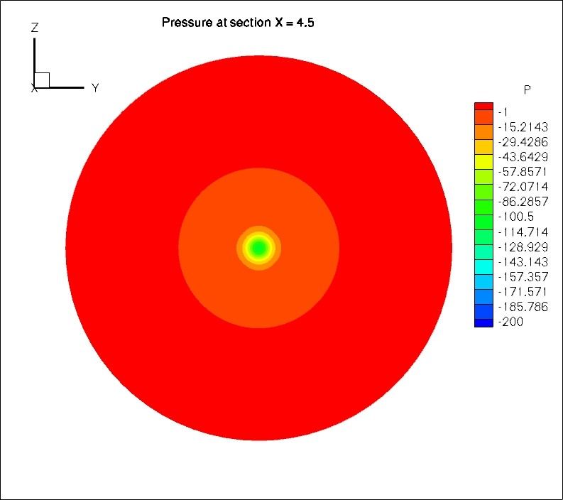
We are interested in studying the effect of refinement criteria in reducing the
discretization error. As vortex flow problems have a singularity in the centre of the vortex
and are not smooth, it is difficult to estimate the error and instead the pressure integral
value at a surface can be an alternate in analyzing the performance of a refinement
criterion because the pressure integral goes to minus infinity for the exact solution, so for
the numerical solutions, lower pressure integral value will correspond to better
performance. So we calculate the pressure integral value at a cross section close to the
outlet of the cylinder at x = 4.5m. We start with flow computations on the uniform grids
first; four grids ranging from coarse to very fine are used and the pressure integral is
computed at the cross section near the outlet. The results are given in the table 3.1.
Pressure Integral at X-
No of cells
section x= 4.5
4.4 × 10³ -7.58 × 10⁻¹
3.4 ×10⁴ -8.9 × 10⁻¹
2.7 × 10⁵ -1.06
2.1× 10⁶ -1.132
Table 3.1: Uniform grids data.
21Figure 3.2:The coarse 4.4K cell Uniform grid cross section (left) with vortex on the right.
Figure 3.3: The refined 2.1M cells uniform grid and pressure contour at X-section x=4.5.
The next step is to go for adaptive grid refinement using the three refinement criteria. We
take an initial grid having 4.4 × 10³ cells and perform adaptive grid refinement controlled
by threshold values and the number of generations. Threshold values are determined by
the number of cells which should be initially marked for refinement or de-refinement.
Higher the number of cells chosen for refinement, more refined the grid will be and vice
versa. In this way, for a particular criterion, we try different threshold values and
eventually select one which will give that desired number of cells marked for
refinement/de-refinement. In order to compare refinement criteria, the threshold values
are set so that number of cells initially selected to be refined/de-refined are equal for each
criteria. In this way we can compare which criterion gives the minimum number of cells
after to reach a particular pressure integral value. The data is tabulated and plotted in the
tables 3.2 to 3.4.
22Threshold No of No of Pressure
value generations cells Integral
0.1 1 1.5×10⁴ -8.70×10⁻¹
2 5×10⁴ -9.85×10⁻¹
3 1.7×10⁵ -1.11
4 5.77×10⁵ -1.194
0.3 1 1×10⁴ -8.71×10⁻¹
2 2.6×10⁴ -9.54×10⁻¹
3 7.6×10⁴ -1.08
4 2.5×10⁵ -1.165
0.4 1 9.2×10³ -8.72×10⁻¹
2 2.3×10⁴ -9.56×10⁻¹
3 6.5×10⁴ -1.08
4 2×10⁵ -1.54
0.7 1 7.4×10³ -9.1×10⁻¹
2 1.6×10⁴ -9.94×10⁻¹
3 4.3×10⁴ -1.10
4 1.3×10⁵ -1.19
Table 3.2: Automatic grid refinement data for velocity gradient criterion.
Threshold No of No of Pressure
value generations cells Integral
0.3 1 1×10⁴ -8.54×10⁻¹
2 1.9×10⁴ -9.70×10⁻¹
4
3 4.3×10 -1.114
4 1.2×10⁵ -1.135
3
0.4 1 8.5×10 -8.58×10-1
4
2 1.9×10 -9.62×10-1
3 4.1×10⁴ -1.11
4 1×10⁵ -1.2
3
0.5 1 8×10 -8.18×10-1
4
2 1.8×10 -9.65×10-1
3 3.8×10⁴ -1.15
5
4 1×10 -1.19
0.9 1 7.4×10³ -9.43×10⁻¹
2 1.3×10⁴ -9.72×10⁻¹
4
3 3.3×10 -1.132
4
4 8.6×10 -1.24
Table 3.3: Automatic grid refinement data for vorticity criterion.
23Threshold No of No of Pressure
value generations cells Integral
18 1 1×10⁴ -8.61×10⁻¹
2 3×10⁴ -9.44×10⁻¹
3 1×10⁵ -1.06
4 4×10⁵ -1.14
45 1 8.8×10³ -8.66×10⁻¹
2 2.2×10⁴ -9.7×10⁻¹
3 6.4×10⁴ -1.092
4 2.4×10⁵ -1.145
53 1 8.3×10³ -8.68×10⁻¹
2 2.1×10⁴ -9.67×10⁻¹
3 6×10⁴ -1.09
4 2.3×10⁵ -1.19
64 1 7.9×10³ -8.57×10⁻¹
2 1.9×10⁴ -9.84×10⁻¹
3 5.9×10⁴ -1.11
4 2×10⁵ -1.20
Table 3.4: Automatic grid refinement data for pressure gradient criterion.
The data given in the tables above is plotted in figures 3.4 to 3.6. We note that all the
three criteria are capturing the flow features and identify the zones for refinement. The
criteria also respond to the threshold values correctly i.e. increasing the threshold value
decreases the number of cells to be refined. The mesh refinement using the criteria also
results in much lower number of cells than that of uniform refinement for a given
pressure integral value. Figures 3.8 and 3.9 show the adapted grids for various grid
generations. All the criteria are able to produce smooth refinement.
24Figure 3.4: Pressure integral plot for velocity gradient criterion at x = 4.5.
Figure 3.5: Pressure integral plot for pressure gradient criterion at x = 4.5.
25Figure 3.6: Pressure integral plot for vorticity criterion at x = 4.5.
Figure 3.7: Pressure integral plot for three criteria at x = 4.5 for maximum threshold.
26Figure 3.8: Effect of number of generations on the refinement for velocity gradient
criteria.
27Figure 3.9: Pressure contours for velocity gradient criterion at maximum threshold for
four generations.
284 KVLCC2 Test Case
In the previous chapter we analyzed the behavior of various refinement criteria for a
simple vortex flow in a cylinder and established that all the criteria were identifying the
refinement areas and capturing vortices by varying degree of accuracy. Now we analyze
these error indicators with more complex test cases. The aim is to check these criteria in
different conditions such as varying turbulence models and effect of the boundary layer
refinement.
As the focus in this project is on the capturing of vortices we analyze the bilge vortices
behind a ship in this section and check the ability of the criteria to predict such vortices
accurately. Traditionally, the interest in the wake flows has been focused on the so-called
“hooks” in the propeller plane which are zones of low axial velocity. The presence of
strong vorticity is responsible for the creation of such hooks.
For this purpose the KVLCC2 test case is chosen. This test case has been extensively
analyzed in the past and a very detailed data are now available and secondly the hooks
discussed above are particularly present as shown by the experimental data. So predicting
such hooks along with the other flow features with the refinement criteria is of particular
importance in this section.
4.1 Geometry and conditions
The original hull form KVLCC2 was conceived by Korean Institute of Ships and Ocean
Engineering (KRISO) to provide data for both explication of flow physics and CFD
validation for a modern tanker ship with bulbous bow. The main features of the ship at
model scale level are given below [4]:
Length between perpendiculars LPP = 5.5172 m
Breadth B / LPP = 0.1813
Draft d / LPP = 0.0650
Wetted surface area, S0 / LPP2 = 0.2656
Block coefficient Cb = 0.8098
Reynolds number Re = 4.6 × 10⁶
Figure 4.1: KVLCC2 scale model.
294.2 Computations
Computations are started from a very coarse mesh, to see if the refinement criterion is
able to effectively create an entire fine mesh. The initial grid has 60 K cells. The three
criteria use three threshold values and three number of generation for each threshold. The
third criteria is restricted to two generation only due to high computational cost and CPU
time in case of three no of generations. The initial computations are performed using the
k-ω SST turbulence model. We can choose, in ISIS-CFD, whether to perform boundary
layer refinement or not. If we opt for boundary layer refinement, cells in the boundary
layers in the directions normal to the wall will be refined only. Here the boundary layer
refinement is also carried out. The threshold values and the grid size data is presented in
the tables 4.1, 4.2 and 4.3.
Threshold value No of generations No of cells after refinement
4.35 1 9.8 × 10⁴
2 1 × 10⁵
3 1 × 10⁵
3.5 1 1.3 × 10⁵
2 1.4 × 10⁵
3 1.4 × 10⁵
4.4 × 10⁻¹ 1 1.9 × 10⁵
2 6.3 × 10⁵
Table 4.1: Automatic grid refinement data for velocity gradient criterion
Threshold value No of generations No of cells after refinement
4.35 1 9.8 × 10⁴
2 1 × 10⁵
3 1 × 10⁵
3.5 1 1.3 × 10⁵
2 1.4 × 10⁵
3 1.4 × 10⁵
-1
4.4 × 10 1 1.8 × 10⁵
2 6.2 × 10⁵
Table 4.2: Automatic grid refinement data for vorticity criterion
Threshold value No of generations No of cells after refinement
8.2 1 1.1 × 10⁵
2 2.3 × 10⁵
3 4.5 × 10⁵
18 1 1.6 × 10⁵
2 4.1 × 10⁵
3 9.7 × 10⁵
35 1 2.2 × 10⁵
2 8 × 10⁵
Table 4.3: Automatic grid refinement data for pressure gradient criterion
304.3 Results
4.3.1. Effect of the boundary layer refinement
Meshes and velocity field contours at the propeller plane are given in figures 4.2 to 4.10.
Plots are for the three refinement criteria with different threshold and no of generations.
If we look at the refined mesh of first two thresholds in case of velocity gradient and
vorticity criteria we see that there is no significant refinement in the propeller plane as
compared to initial mesh. The pressure gradient criterion performs better than the other
two. The main reason behind this phenomenon is that the velocity gradients and the
vorticity are high in the boundary layer region. If we go for boundary layer refinement
the two criteria respond to this zone which results in the unnecessary and costly
refinement in the boundary layer and little refinement in the other regions. On the other
hand, the pressure gradient criterion avoids such refinement in the boundary layer
because the pressure varies little in that zone. The boundary layer is only refined there,
where it is dictated by the outside flow. This is the main advantage of the pressure
gradient criteria over the other two and results in more accurate flow features predictions.
The boundary layer refinement effect is also depicted in the refined grid size resulting
form various number of generations. A kind of saturation phenomenon occurs here. As
shown in the tables 4.1, 4.2 and 4.3, we see that for the velocity gradient and vorticity
criteria, the first two thresholds have very little increase in the grid size going from one
number of generations to three. So for higher threshold values, the number of generations
becomes insignificant. The pressure gradient criterion does not follow such trend and
there is a significant increase in the number of cells if we increase the number of
generations for a particular threshold value. The threshold value being very low in case of
third threshold, allows the velocity gradient and vorticity criteria to refine the zones out
of the boundary layer as well.
Limiting streamlines are also shown in the figures for various refinement criteria and
conditions. All criteria, generally, follow the same pattern: the upper lines move
backwards all the way onto the upper part of the stern. The lines start to move downward
at about mid girth and become more vertical approaching the stern. Near the bilge the
lines moving downward meet the lines from bottom and here a vortex type separation
occurs and the created vortex sheet rolls up into the bilge vortex.
Among the three criteria, the hook shape in the propeller plane is best captured by the
pressure gradient criteria due to the reasons explained above. As the turbulence model
used here is k-ω SST, later in the section it will be shown that the EASM turbulence
model performs even better than the k-ω SST model and accurately captures the hook
shape.
31Figure 4.2: Velocity gradient criterion for 1st threshold and 3 generations. Propeller plane
Mesh and axial velocity contour. Original mesh is on left and refined mesh on right.
Figure 4.3: Velocity gradient criterion for 2nd threshold and 3 generations. Propeller plane
Mesh and axial velocity contour. Original mesh is on left and refined mesh on right.
32Figure 4.4: Velocity gradient criterion for 3rd threshold and 2 generations. Propeller plane
Mesh, axial velocity contour, cross flow vectors and streamlines.
33Figure 4.5: Vorticity criterion for 1st threshold and 3 generations. Propeller plane Mesh
and axial velocity contour. Original mesh is on left and refined mesh on right.
Figure 4.6: Vorticity criterion for 2nd threshold and 3 generations. Propeller plane Mesh
and axial velocity contour. Original mesh is on left and refined mesh on right.
34You can also read