ARSM: Augment-REINFORCE-Swap-Merge Estimator for Gradient Backpropagation Through Categorical Variables
←
→
Page content transcription
If your browser does not render page correctly, please read the page content below
ARSM: Augment-REINFORCE-Swap-Merge Estimator for
                Gradient Backpropagation Through Categorical Variables

                                  Mingzhang Yin * 1 Yuguang Yue * 1 Mingyuan Zhou 2

                         Abstract                              zk ∈ {1, 2, . . . , C} as a univariate C-way categorical vari-
                                                               able, and z = (z1 , . . . , zK ) ∈ {1, 2, . . . , C}K as a K-
      To address the challenge of backpropagating              dimensional C-way multivariate categorical vector. In dis-
      the gradient through categorical variables, we           crete latent variable models, K will be the dimension of
      propose the augment-REINFORCE-swap-merge                 the discrete latent space, each dimension of which can be
      (ARSM) gradient estimator that is unbiased               further represented as a C-dimensional one-hot vector. In
      and has low variance. ARSM first uses vari-              RL, C represents the size of the discrete action space and
      able augmentation, REINFORCE, and Rao-                   z is a sequence of discrete actions from that space. In even
      Blackwellization to re-express the gradient as an        more challenging settings, one may have a sequence of K-
      expectation under the Dirichlet distribution, then       dimensional C-way multivariate categorical vectors, which
      uses variable swapping to construct differently          appear both in categorical latent variable models with mul-
      expressed but equivalent expectations, and finally       tiple stochastic layers, and in RL with a high dimensional
      shares common random numbers between these               discrete action space or multiple agents, which may consist
      expectations to achieve significant variance reduc-      of as many as C K unique combinations at each time step.
      tion. Experimental results show ARSM closely
      resembles the performance of the true gradient for       With f (z) and qφ (z) denoted as the reward function and dis-
      optimization in univariate settings; outperforms         tribution for categorical z, respectively, we need to optimize
      existing estimators by a large margin when ap-           parameter φ to maximize the expected reward as
      plied to categorical variational auto-encoders; and                        R
      provides a “try-and-see self-critic” variance reduc-             E(φ) = f (z)qφ (z)dz = Ez∼qφ (z) [f (z)].          (1)
      tion method for discrete-action policy gradient,
      which removes the need of estimating baselines           Here we consider both categorical latent variable models
      by generating a random number of pseudo actions          and policy optimization for discrete actions, which arise in a
      and estimating their action-value functions.             wide array of real-world applications. A number of unbiased
                                                               estimators for backpropagating the gradient through discrete
                                                               latent variables have been recently proposed (Tucker et al.,
                                                               2017; Grathwohl et al., 2018; Yin & Zhou, 2019; Andriyash
1. Introduction                                                et al., 2018). However, they all mainly, if not exclusively,
The need to maximize an objective function, expressed          focus on the binary case (i.e., C = 2). The categorical case
as the expectation over categorical variables, arises in a     (i.e., C ≥ 2) is more widely applicable but generally much
wide variety of settings, such as discrete latent variable     more challenging. In this paper, to optimize the objective in
models (Zhou, 2014; Jang et al., 2017; Maddison et al.,        (1), inspired by the augment-REINFORCE-merge (ARM)
2017) and policy optimization for reinforcement learning       gradient estimator restricted for binary variables (Yin &
(RL) with discrete actions (Sutton & Barto, 1998; Weaver       Zhou, 2019), we introduce the augment-REINFORCE-swap-
& Tao, 2001; Schulman et al., 2015; Mnih et al., 2016;         merge (ARSM) estimator that is unbiased and well controls
Grathwohl et al., 2018). More specifically, let us denote      its variance for categorical variables.
  *
   Equal contribution 1 Department of Statistics and Data      The proposed ARSM estimator combines variable augmen-
Sciences, 2 Department of IROM, McCombs School of              tation (Tanner & Wong, 1987; Van Dyk & Meng, 2001),
Business, The University of Texas at Austin, Austin,           REINFORCE (Williams, 1992) in an augmented space, Rao-
TX 78712, USA. Correspondence to: Mingyuan Zhou                Blackwellization (Casella & Robert, 1996), and a merge step
.                            that shares common random numbers between different but
Proceedings of the 36 th International Conference on Machine   equivalent gradient expectations to achieve significant vari-
Learning, Long Beach, California, PMLR 97, 2019. Copyright     ance reduction. While ARSM with C = 2 reduces to the
2019 by the author(s).                                         ARM estimator (Yin & Zhou, 2019), whose merge step can
ARSM: Augment-REINFORCE-Swap-Merge Gradient for Categorical Variables
be realized by applying antithetic sampling (Owen, 2013) trol variates, also known as baselines (Williams, 1992), into
in the augmented space, the merge step of ARSM with the expectation in (2) before performing Monte Carlo inte-
C > 2 cannot be realized in this manner. Instead, ARSM gration (Paisley et al., 2012; Ranganath et al., 2014; Mnih &
requires distinct variable-swapping operations to construct Gregor, 2014; Gu et al., 2016; Mnih & Rezende, 2016; Ruiz
differently expressed but equivalent expectations under the et al., 2016; Kucukelbir et al., 2017; Naesseth et al., 2017).
Dirichlet distribution before performing its merge step. For discrete z, Tucker et al. (2017) and Grathwohl et al.
(2018) improve REINFORCE by introducing continuous
Experimental results on both synthetic data and several rep-
relaxation based baselines, whose parameters are optimized
resentative tasks involving categorical variables are used
by minimizing the sample variance of gradient estimates.
to illustrate the distinct working mechanism of ARSM. In
particular, our experimental results on latent variable mod-
els with one or multiple categorical stochastic hidden lay- 2. ARSM Gradient For Categorical Variables
ers show that ARSM provides state-of-the-art training and
Let us denote z ∼ Cat(σ(φ)) as a categorical variable such
out-of-sample prediction performance. Our experiments PC φ
on RL with discrete action spaces show that ARSM pro- that P (z = c | φ) = σ(φ)c = eφc i=1 e , where φ :=
i
C
(φ1 , . . . , φC ) and σ(φ) := (eφ1 , . . . , eφC )/ i=1 eφi is the
P
vides a “try-and-see self-critic” method to produce unbi-
ased and low-variance policy gradient estimates, removing softmax function. For the expectated reward defined as
the need of constructing baselines by generating a random PC
E(φ) := Ez∼Cat(σ(φ)) [f (z)] = i=1 f (i)σ(φ)i ,
number of pseudo actions at a given state and estimating
their action-value functions. These results demonstrate the the gradient can be expressed analytically as
effectiveness and versatility of the ARSM estimator for
gradient backpropagation through categorical stochastic lay- ∇φc E(φ) = σ(φ)c f (c) − σ(φ)c E(φ) (3)
ers. Python code for reproducible research is available at
https://github.com/ARM-gradient/ARSM. or expressed with REINFORCE as
∇φc E(φ) = Ez∼Cat(σ(φ)) f (z)(1[z=c] − σ(φ)c ) , (4)
1.1. Related Work
For optimizing (1) for categorical z, the difficulty lies in where 1[·] is an indicator function that is equal to one if the
developing a low-variance and preferably unbiased estima- argument is true and zero otherwise. However, the analytic
tor for its gradient with respect to φ, expressed as ∇φ E(φ). expression quickly becomes intractable for a multivariate
An unbiased but high-variance gradient estimator that is uni- setting, and the REINFORCE estimator often comes with
versally applicable to (1) is REINFORCE (Williams, 1992). significant estimation variance. While the ARM estimator
Using the score function ∇φ log qφ (z) = ∇φ qφ (z)/qφ (z), of Yin & Zhou (2019) is unbiased and provides significant
REINFORCE expresses the gradient as an expectation as variance reduction for binary variables, it is restricted to
C = 2 and hence has limited applicability.
∇φ E(φ) = Ez∼qφ (z) [f (z)∇φ log qφ (z)], (2)
Below we introduce the augment-REINFORCE (AR), AR-
and approximates it with Monte Carlo integration (Owen, swap (ARS), and ARS-merge (ARSM) estimators for a
2013). However, the estimation variance with a limited univariate C-way categorical variable, and later generalize
number of Monte Carlo samples is often too high to make them to multivariate, hierarchical, and sequential settings.
vanilla REINFORCE a sound choice for categorical z.
To address the high-estimation-variance issue for categori- 2.1. AR: Augment-REINFORCE
cal z, one often resorts to a biased gradient estimator. For Let us denote π := (π1 , . . . , πC ) ∼ Dir(1C ) as a Dirichlet
example, Maddison et al. (2017) and Jang et al. (2017) re- distribution whose C parameters are all ones. We first state
lax the categorical variables with continuous ones and then three statistical properties that can directly lead to the pro-
apply the reparameterization trick to estimate the gradients, posed AR estimator. We describe in detail in Appendix A
reducing variance but introducing bias. Other biased estima- how we actually arrive at the AR estimator, with these prop-
tors for backpropagating through binary variables include erties obtained as by-products, by performing variable aug-
the straight-through estimator (Hinton, 2012; Bengio et al., mentation, REINFORCE, and Rao-Blackwellization. Thus
2013) and the ones of Gregor et al. (2014); Raiko et al. we are in fact reverse-engineering our original derivation of
(2014); Cheng et al. (2018). With biased gradient estimates, the AR estimator to help concisely present our findings.
however, a gradient ascent algorithm may not be guaranteed
to work, or may converge to unintended solutions. Property I. The categorical variable z ∼ Cat(σ(φ)) can be
equivalently generated as
To keep REINFORCE unbiased while sufficiently reducing
its variance, a usual strategy is to introduce appropriate con- z := arg mini∈{1,...,C} πi e−φi , π ∼ Dir(1C ).ARSM: Augment-REINFORCE-Swap-Merge Gradient for Categorical Variables
Property II. E(φ) = Eπ∼Dir(1C ) [f (arg mini πi e−φi )]. properties: z c j = z j c and z c j = z if c = j, and the
Property III. Eπ∼Dir(1C ) [f (arg mini πi e−φi )Cπc ] = number of unique values in {z c j }c,j that are different from
E(φ) + σ(φ)c E(φ) − σ(φ)c f (c). the true action z is between 0 and C − 1.
These three properties, Property III in particular, are pre- With (3), we have another useful property as
viously unknown to the best of our knowledge. They are PC
Property V. c=1 ∇φc E(φ) = 0.
directly linked to the AR estimator shown below.
Combining it with the estimator in (6) leads to
Theorem 1 (AR estimator). The gradient of E(φ) =
Ez∼Cat(σ(φ)) [f (z)], as shown in (3), can be re-expressed PC
Eπ∼Dir(1C ) C1 c=1 gAR (π c j )c = 0.
(7)
as an expectation under a Dirichlet distribution as
PC
∇φc E(φ) = Eπ∼Dir(1C ) [gAR (π)c ], Thus we can utilize C1 c=1 gAR (π c j )c as a baseline func-
tion that is nonzero in general but has zero expectation under
gAR (π)c : = f (z)(1 − Cπc ), (5) π ∼ Dir(1C ). Subtracting (7) from (6) leads to another un-
−φi
z : = arg mini∈{1,...,C} πi e . biased estimator, with category j as the reference, as
∇φc E(φ) = Eπ∼Dir(1C ) [gARS (π, j)c ],
Distinct from REINFORCE in (4), the AR estimator in (5) PC
now expresses the gradient as an expectation under a Dirich- gARS (π, j)c := gAR (π c j )c − C1 m=1 gAR (π m j
)m , (8)
let distributed random noise. From this point of view, it is PC
= f (z c j ) − C1 m=1 f (z m j ) (1 − Cπj ),
somewhat related to the reparameterization trick (Kingma &
Welling, 2013; Rezende et al., 2014), which is widely used which is referred to as the AR-swap (ARS) estimator, due
to express the gradient of an expectation under reparame- to the use of variable-swapping in its derivation from AR.
terizable random variables as an expectation under random
noises. Thus one may consider AR as a special type of repa- 2.3. ARSM: Augment-REINFORCE-Swap-Merge
rameterization gradient, which, however, requires neither z
to be reparameterizable nor f (·) to be differentiable. For ARS in (8), when the reference category j is randomly
chosen from {1, . . . , C} and hence is independent of π
2.2. ARS: Augment-REINFORCE-Swap and φ, it is unbiased. Furthermore, we find that it can be
further improved, especially when C is large, by adding a
Let us swap the mth and jth elements of π to define vector merge step to construct the ARS-merge (ARSM) estimator:
πm j
:= (π1m j m
, . . . , πC j
), Theorem 2 (ARSM estimator). The gradient of E(φ) =
Ez∼Cat(σ(φ)) [f (z)] with respect to φc , can be expressed as
m j
where πm = πj , πjm j = πm , and ∀ c ∈ / {m, j},
m j
πc = πc . Another property to be repeatedly used is: ∇φc E(φ) = Eπ∼Dir(1C ) gARSM (π)c ,
PC
Property IV. If π ∼ Dir(1C ), then π m j
∼ Dir(1C ). gARSM (π)c := C1 j=1 gARS (π, j)c (9)
PC c j C
= j=1 f (z ) − C1 m=1 f (z m j ) ( C1 − πj ).
P
This leads to a key observation for the AR estimator in (5):
swapping any two variables of the probability vector π in-
side the expectation does not change the expected value. Note ARSM requires C(C − 1)/2 swaps to generate pseudo
Using the idea of sharing common random numbers be- actions, the unique number of which that differ from z is be-
tween different expectations to potentially significantly re- tween 0 and C − 1; a naive implementation requires O(C 2 )
duce Monte Carlo integration variance (Owen, 2013), we arg min operations, which, however, is totally unnecessary,
propose to swap πc and πj in (5), where j ∈ {1, . . . , C} is as in general it can at least be made below O(2C) and hence
a reference category chosen independently of π and φ. This is scalable even C is very large (e.g., C = 10, 000); please
variable-swapping operation changes the AR estimator to see Appendix B and the provided code for more details.
Note if all pseudo actions z c j are the same as the true
∇φc E(φ) = Eπ∼Dir(1C ) [gAR (π c j )c ] action z, then the gradient estimates will be zeros for all φc .
gAR (π c j )c : = f (z c j )(1 − Cπj ), (6) Corollary 3. When C = 2, both the ARS estimator in (8)
c j −φi
z c j
: = arg mini∈{1,...,C} πi e , and ARSM estimator in (9) reduce to the unbiased binary
ARM estimator introduced in Yin & Zhou (2019).
where we have applied identity πcc j = πj and Property IV.
We refer to z defined in (5) as the “true action,” and z c j Detailed derivations and proofs are provided in Appendix A.
defined in (6) as the cth “pseudo action” given j as the refer- Note for C = 2, Proposition 4 of Yin & Zhou (2019) shows
ence category. Note the pseudo actions satisfy the following that the ARM estimator is the AR estimator combined withARSM: Augment-REINFORCE-Swap-Merge Gradient for Categorical Variables
an optimal baseline that is subject to an anti-symmetric con- discounted state visitation frequency, the policy gradient via
straint. When C > 2, however, such type of theoretical REINFORCE (Williams, 1992) can be expressed as
analysis becomes very challenging for both the ARS and
ARSM estimators. For example, it is even unclear how to ∇θ J(θ) = Eat ∼πθ (at |st ), st ∼ρπ (s) [∇θ ln πθ (at |st )Q(st , at )].
define anti-symmetry for categorical variables. Thus in what
For variance reduction, one often subtracts state-dependent
follows we will focus on empirically evaluating the effec-
baselines b(st ) from Q̂(st , at ) (Williams, 1992; Greensmith
tiveness of both ARS and ARSM for variance reduction.
et al., 2004). In addition, several different action-dependent
baselines b(st , at ) have been recently proposed (Gu et al.,
3. ARSM Estimator for Multivariate, 2017; Grathwohl et al., 2018; Wu et al., 2018; Liu et al.,
Hierarchical, and Sequential Settings 2018), though their promise in appreciable variance reduc-
tion without introducing bias for policy gradient has been
This section shows how the proposed univariate ARS and questioned by Tucker et al. (2018).
ARSM estimators can be generalized into multivariate, hier-
archical, and sequential settings. We summarize ARS and Distinct from all previous baseline-based variance reduction
ARSM (stochastic) gradient ascent for various types of cate- methods, in this paper, we develop both the ARS and ARSM
gorical latent variables in Algorithms 1-3 of the Appendix. policy gradient estimators, which use the action-value func-
tions Q(st , at ) themselves combined with pseudo actions
3.1. ARSM for Multivariate Categorical Variables and to achieve variance reduction:
Stochastic Categorical Network Proposition 4 (ARS/ARSM policy gradient). The policy
gradient ∇θ J(θ) can be expressed as
We generalize the univariate AR/ARS/ARSM estimators
to multivariate ones, which can backpropagate the gradi- ∇θ J(θ) = E$t ∼Dir(1C ), st ∼ρπ (s) ∇θ C
P
(10)
c=1 gtc φtc ,
ent through a K dimensional vector of C-way categorical
variables as z = (z1 , . . . , zK ), where zk ∈ {1, . . . , C}. where $ t = ($t1 , . . . , $tC )0 and φtc is the cth element of
We further generalize them to backpropagate the gradient φt = Tθ (st ) ∈ RC ; under the ARS estimator, we have
through multiple stochastic categorical layers, the tth layer c jt
of which consists of a Kt -dimensional C-way categorical gtc : = ft∆ ($ t )(1 − C$tjt ),
vector as z t = (zt1 , . . . , ztKt )0 ∈ {1, . . . , C}Kt . We defer
PC
ft∆ ($ t ) : = Q(st , act jt ) − C1 m=1 Q(st , am
c jt
t
jt
),
all the details to Appendix C due to space constraint. c jt c jt −φti
at : = arg mini∈{1,...,C} $ti e ,
Note for categorical variables, especially in multivariate (11)
and/or hierarchical settings, the ARS/ARSM estimators may
appear fairly complicated due to their variable-swapping where jt ∈ {1, . . . , C} is a randomly selected reference
operations. Their implementations, however, are actually category for time step t; under the ARSM estimator, we have
relatively straightforward, as shown in Algorithms 1 and 2 PC
of the Appendix, and the provided Python code. gtc := j=1 ft∆ c j
($ t )( C1 − $tj ). (12)
3.2. ARSM for Discrete-Action Policy Optimization Note as the number of unique actions among am t
j
is as
few as one, in which case the ARS/ARSM gradient is zero
In RL with a discrete action space with C possible ac- and there is no need at all to estimate the Q function, and
tions, at time t, the agent with state st chooses action as many as C, in which case one needs to estimate the Q
at ∈ {1, . . . , C} according to policy function C times. Thus if the computation of estimating
πθ (at | st ) := Cat(at ; σ(φt )), φt := Tθ (st ), Q once is O(1), then the worst computation for an episode
that lasts T time steps before termination is O(T C). Usu-
where Tθ (·) denotes a neural network parameterized by θ; ally the number of distinct pseudo actions will decrease
the agent receives award r(st , at ) at time t, and state st dramatically as the training progresses. We illustrate this
transits to state st+1 according to P(st+1 | st , at ). With in Figure 7, where we show the trace of categorical vari-
discount parameter γ ∈ (0, 1], policy gradient methods able’s entropy and number of distinct pseudo actions that
optimize P∞θ to maximize the expected reward J(θ) = differ from the true action. Examining (11) and (12) shows
EP,πθ [ t=0 γ t r(st , at )] (Sutton & Barto, 1998; Sutton that the ARS/ARSM policy gradient estimator can be in-
et al., 2000; Peters & Schaal, 2008; P∞ Schulman et al., tuitively understood as a “try-and-see self-critic” method,
0
2015). With Q(st , at ) := EP,πθ [ t0 =t γ t −t r(st0 , at0 )] which eliminates the need of constructing baselines and es-
denoted
P∞ t0as the action-value functions, Q̂(st , at ) := timating their parameters for variance reduction. To decide
−t
t0 =t γ P∞ t , at ) as their sample estimates, and
r(s 0 0 the gradient direction of whether increasing the probability
ρπ (s) := t=0 γ t P(st = s | s0 , πθ ) as the unnormalized of action c at a given state, it compares the pseudo-actionARSM: Augment-REINFORCE-Swap-Merge Gradient for Categorical Variables
reward Q(st , act j ) with the average of all pseudo-action which has been shown in Yin & Zhou (2019) to outperform
rewards {Q(st , am t
j
)}m=1,C . If the current policy is very a wide variety of estimators for binary variables, including
confident on taking action at at state st , which means φtat the REBAR estimator of Tucker et al. (2017). The true
dominates the other C − 1 elements of φt = Tθ (st ), then it gradient in this example can be computed analytically as
is very likely that am
t
jt
= at for all m, which will lead to in (3). All estimators in comparison use a single Monte
zero gradient at time t. On the contrary, if the current policy Carlo sample for gradient estimation. We initialize φc = 0
is uncertain about which action to choose, then more pseudo for all c and fix the gradient-ascent stepsize as one.
actions that are different from the true action are likely to be
As shown in Figure 1, without appropriate variance reduc-
generated. This mechanism encourages exploration when
tion, both AR and REINFORCE either fail to converge or
the policy is uncertain, and balance the tradeoff of explo-
converge to a low-reward solution. We notice RELAX for
ration and exploitation intrinsically. It also explains our
C = R = 30 is not that stable across different runs; in
empirical observations that ARS/ARSM tends to generate a
this particular run, it manages to obtain a relatively high re-
large number of unique pseudo actions in the early stages
ward, but its probabilities converge towards a solution that is
of training, leading to fast convergence, and significantly re-
different from the optimum σ(φ) = (0, . . . , 0, 1). By con-
duced number once the policy becomes sufficiently certain,
trast, Gumbel-Softmax, ARS, and ARSM all robustly reach
leading to stable performance after convergence.
probabilities close to the optimum σ(φ) = (0, . . . , 0, 1) af-
ter 5000 iterations across all random trials. The gradient
4. Experimental Results variance of ARSM is about one to four magnitudes less
than these of the other estimators, which helps explain why
In this section, we use a toy example for illustration, demon-
ARSM is almost identical to the true gradient in moving
strate both multivariate and hierarchical settings with cate-
σ(φ) towards the optimum that maximizes the expected
gorical latent variable models, and demonstrate the sequen-
reward. The advantages of ARSM become even clearer in
tial setting with discrete-action policy optimization. Com-
more complex settings where analytic gradients become
parison of gradient variance between various algorithms can
intractable to compute, as shown below.
be found in Figures 1 and 3-6.
4.2. Categorical Variational Auto-Encoders
4.1. Example Results on Toy Data
For optimization involving expectations with respect to mul-
To illustrate the working mechanism of the ARSM estimator,
tivariate categorical variables, we consider a variational
we consider learning φ ∈ RC to maximize
auto-encoder (VAE) with a single categorical stochastic
Ez∼Cat(σ(φ)) [f (z)], f (z) := 0.5 + z/(CR), (13) hidden layer. We further consider a categorical VAE with
two categorical stochastic hidden layers to illustrate opti-
where z ∈ {1, . . . , C}. The optimal solution is σ(φ) = mization involving expectations with respect to hierarchical
(0, . . . , 0, 1), which leads to the maximum expected reward multivariate categorical variables.
of 0.5 + 1/R. The larger the C and/or R are, the more
challenging the optimization becomes. We first set C = Following Jang et al. (2017), we consider a VAE with a
R = 30 that are small enough to allow existing algorithms categorical hidden layer to model D-dimensional binary
to perform reasonably well. Further increasing C or R will QDdecoder parameterized by θ is expressed
observations. The
often fail existing algorithms and ARS, while ARSM always as pθ (x | z) = i=1 pθ (xi | z), where z ∈ {1, . . . , C}K is
performs almost as good as the true gradient when used in a K-dimensional C-way categorical vector and pθ (xi | z)
optimization via gradient ascent. We include the results for encoder parameterized by φ
is Bernoulli distributed. The Q
K
C = 1, 000 and 10, 000 in Figures 4 and 5 of the Appendix. is expressed as qφ (z | x) = k=1 qφ (zk | x). We set the
prior as p(zk = c) = 1/C for all c and k. For optimization,
We perform an ablation study of the proposed AR, ARS, we maximize the evidence lower bound (ELBO) as
and ARSM estimators. We also make comparison to two | z)p(z)
L(x) = Ez∼qφ (z | x) ln pθq(x
representative low-variance estimators, including the bi- φ (z | x) . (14)
ased Gumbel-Softmax estimator (Jang et al., 2017; Maddi-
son et al., 2017) that applies the reparameterization trick We also consider a two-categorical-hidden-layer VAE,
after continuous relaxation of categorical variables, and whose encoder and decoder are constructed as
the unbiased RELAX estimator of Grathwohl et al. (2018) qφ1:2 (z 1 , z 2 | x) = qφ1 (z 1 | x)qφ2 (z 2 | z 1 ),
that combines reparameterization and REINFORCE with an
pθ1:2 (x | z 1 , z 2 ) = pθ1 (x | z 1 )pθ2 (z 1 | z 2 ),
adaptively estimated baseline.
PC We compare them in terms
of the expected reward as c=1 σ(φ)c f (c), gradients for where z 1 , z 2 ∈ {1, . . . , C}K . The ELBO is expressed as
φc , probabilities σ(φ)c , and gradient variance. Note when h pθ 1 (x | z 1 )pθ 2 (z 1 | z 2 )p(z 2 )
i
L(x) = Eqφ1:2 (z1 ,z2 | x) ln qφ1 (z 1 | x)qφ2 (z 2 | z 1 )
. (15)
C = 2, both ARS and ARSM reduce to the ARM estimator,ARSM: Augment-REINFORCE-Swap-Merge Gradient for Categorical Variables
Figure 1. Comparison of a variety of gradient estimators in maximizing (13). The optimal solution is σ(φ) = (0, . . . , 1), which means
z = C with probability one. The reward is computed analytically by Ez∼Cat(σ(φ)) [f (z)] with maximum as 0.533. Rows 1, 2, and 3 show
the trace plots of reward E[f (z)], the gradients with respect to φ1 and φC , and the probabilities σ(φ)1 and σ(φ)C , respectively. Row 4
shows the gradient variance estimation with 100 Monte Carlo samples at each iteration, averaged over categories 1 to C.
with a single categorical hidden layer, and modify it with our
best effort for the VAE with two categorical hidden layers;
we modify the RELAX code 2 with our best effort to allow
it to optimize VAE with a single categorical hidden layer.
For the single-hidden-layer VAE, we connect its latent cate-
gorical layer z and observation layer x with two nonlinear
deterministic layers; for the two-hidden-layer VAE, we add
an additional categorical hidden layer z 2 that is linearly
connected to the first one. See Table 3 of the Appendix
for detailed network architectures. In our experiments, all
methods use exactly the same network architectures and
Figure 2. Plots of negative ELBOs (nats) on binarized MNIST
data, set the mini-batch size as 200, and are trained by the
against training iterations (analogous ones against times are shown
in Figure 8). The solid and dash lines correspond to the training Adam optimizer (Kingma & Ba, 2014), whose learning rate
and testing respectively (best viewed in color). is selected from {5, 1, 0.5} × 10−4 using the validation set.
For both categorical VAEs, we set K = 20 and C = 10. The results in Table 1 and Figure 2 clearly show that for
We train them on a binarized MNIST dataset as in van den optimizing the single-categorical-hidden-layer VAE, both
Oord et al. (2017) by thresholding each pixel value at 0.5. ARS and ARSM estimators outperform all the other ones in
Implementations of the VAEs with one and two categori- both training and testing ELBOs. In particular, ARSM out-
cal hidden layers are summarized in Algorithms 1 and 2, performs all the other estimators by a large margin. We also
respectively; see the provided code for more details. consider Gumbel-Softmax by computing its gradient with 25
Monte Carlo samples, making it run as fast as the provided
We consider the AR, ARS, and ARSM estimators, and in- ARSM code does per iteration. In this case, both algorithms
clude the REINFORCE (Williams, 1992), Gumbel-Softmax take similar time but ARSM achieves −ELBOs for the train-
(Jang et al., 2017), and RELAX (Grathwohl et al., 2018) ing and testing sets as 94.6 and 100.6, respectively, while
estimators for comparison. We note that Jang et al. (2017) those of Gumbel-Softmax are 102.5 and 103.6, respectively.
has already shown Gumbel-Softmax outperforms a wide The performance gain of ARSM can be explained by both
variety of previously proposed estimators; see Jang et al. its unbiasedness and a clearly lower variance exhibited by
(2017) and the references therein for more details. its gradient estimates in comparison to all the other estima-
We present the trace plots of the training and validation neg- tors, as shown in Figure 6 of the Appendix. The results on
ative ELBOs in Figure 2 and gradient variance in Figure 6. the two-categorical-hidden-layer VAE, which adds a linear
The numerical values are summarized in Table 1. We use categorical layer on top of the single-categorical-hidden-
the Gumbel-Softmax code 1 to obtain the results of the VAE layer VAE, also suggest that ARSM can further improve its
2
1
https://github.com/ericjang/gumbel-softmax https://github.com/duvenaud/relaxARSM: Augment-REINFORCE-Swap-Merge Gradient for Categorical Variables
Table 1. Comparison of training and testing negative ELBOs (nats) on binarized MNIST between ARSM and various gradient estimators.
Gradient estimator REINFORCE RELAX ST Gumbel-S. AR ARS ARSM Gumbel-S.-2layer ARSM-2layer
−ELBO (Training) 142.4 129.1 112.7 135.8 101.5 94.6 111.4 92.5
−ELBO (Testing) 141.3 130.3 113.4 136.6 106.7 100.6 113.8 99.9
Table 2. Comparison of the test negative log-likelihoods between As shown in Table 2, optimizing a stochastic categorical
ARSM and various gradient estimators in Jang et al. (2017), for network with the ARSM estimator achieves the lowest test
the MNIST conditional distribution estimation benchmark task. negative log-likelihood, outperforming all previously pro-
Gradient estimator ARSM ST Gumbel-S. MuProp posed gradient estimators on the same structured stochastic
− log p(xl | xu ) 58.3 ± 0.2 61.8 59.7 63.0 networks, including straight through (ST) (Bengio et al.,
2013) and ST Gumbel-softmax (Jang et al., 2017) that are
performance by adding more stochastic hidden layers and biased, and MuProp (Gu et al., 2016) that is unbiased.
clearly outperforms the biased Gumbel-Softmax estimator.
4.4. Discrete-Action Policy Optimization
4.3. Maximum Likelihood Estimation for a Stochastic The key of applying the ARSM policy gradient shown
Categorical Network in (12) is to provide, under the current policy πθ , the
Denoting xl , xu ∈ R392 as the lower and upper halves action-value functions’ sample estimates Q̂(st , at ) :=
∞ t0 −t
P
of an MNIST digit, respectively, we consider a standard t0 =t γ r(st0 , at0 ) for all unique values in {act j }c,j .
benchmark task of estimating the conditional distribution Thus ARSM is somewhat related to the vine method pro-
pθ0:2 (xl | xu ) (Raiko et al., 2014; Bengio et al., 2013; Gu posed in Schulman et al. (2015), which defines a heuristic
et al., 2016; Jang et al., 2017; Tucker et al., 2017). We con- rollout policy that chooses a subset of the states along the
sider a stochastic categorical network with two stochastic true trajectory as the “rollout set,” samples K pseudo ac-
categorical hidden layers, expressed as tions uniformly at random from the discrete-action set at
each state of the rollout set, and performs a single roll-
xl ∼ Bernoulli(σ(Tθ0 (b1 ))), out for each state-pseudo-action-pair to estimate its action-
Q20 value function Q. ARSM chooses its rollout set in the same
b1 ∼ c=1 Cat(b1c ; σ(Tθ1 (b2 )[10(c−1)+(1:10)] )), manner, but is distinct from the vine method in having a
Q20
b2 ∼ c=1 Cat(b2c ; σ(Tθ2 (xu )[10(c−1)+(1:10)] )), rigorously derived rollout policy: it swaps the elements
of $ t ∼ Dir(1C ) to generate pseudo actions if state st be-
where both b1 and b2 are 20-dimensional 10-way longs to the rollout set; the number of unique pseudo actions
categorical variables, Tθ (·) denotes linear transform, that are different from the true action at is a random number,
Tθ2 (xu )[10(c−1)+(1:10)] is a 10-dimensional vector consist- which is positively related to the uncertainty of the policy
ing of elements 10(c − 1) + 1 to 10c of Tθ2 (xu ) ∈ R200 , and hence often negatively related to its convergence; and
Tθ1 (b2 ) ∈ R200 , and Tθ0 ∈ R392 . Thus we can con- a single rollout is then performed for each of these unique
sider the network structure as 392-200-200-392, making pseudo actions to estimate its Q.
the results directly comparable with these in Jang et al.
As ARSM requires the estimation of Q function for each
(2017) for stochastic categorical network. We approximate
unique state-pseudo-action pair using Monte Carlo rollout, it
log pθ0:2 (xl | xu ) with K Monte Carlo samples as
could have high computational complexity if (1) the number
1
PK (k) of unique pseudo actions is large, and (2) each rollout takes
log K k=1 Bernoulli(xl ; σ(Tθ0 (b1 ))), (16) many expensive steps (interactions with the environments)
(k) Q20 (k) (k)
before termination. However, there exist ready solutions
where b1 ∼ c=1 Cat(b1c ; σ(Tθ1 (b2 )[10(c−1)+(1:10)] )), and many potential ones. As given a true trajectory, all
(k) Q 20 (k)
b2 ∼ c=1 Cat(b2c ; σ(Tθ 2 (xu )[10(c−1)+(1:10)] )). We
the state-pseudo-action rollouts of ARSM can be indepen-
perform training with K = 1, which can also be considered dently simulated and hence all pseudo-action related Q’s
as optimizing on a single-Monte-Carlo-sample estimate of can be estimated in an embarrassingly parallel manner. Fur-
the lower bound of the log marginal likelihood. We use thermore, in addition to Monte Carlo estimation, we can
Adam (Kingma & Ba, 2014), with the learning rate set as potentially adapt for ARSM a wide variety of off-the-shelf
10−4 , mini-batch size as 100, and number of training epochs action-value function estimation methods (Sutton & Barto,
as 2000. Given the inferred point estimate of θ 0:2 , we 1998), to either accelerate the estimation of Q or further
evaluate the accuracy of conditional density estimation by reduce the variance (though possibly at the expense of intro-
estimating the negative log-likelihood − log pθ0:2 (xl | xu ) ducing bias). In our experiment, for simplicity and clarity,
using (16), averaging over the test set with K = 1000. we choose to use Monte Carlo estimation to obtain Q̂ forARSM: Augment-REINFORCE-Swap-Merge Gradient for Categorical Variables
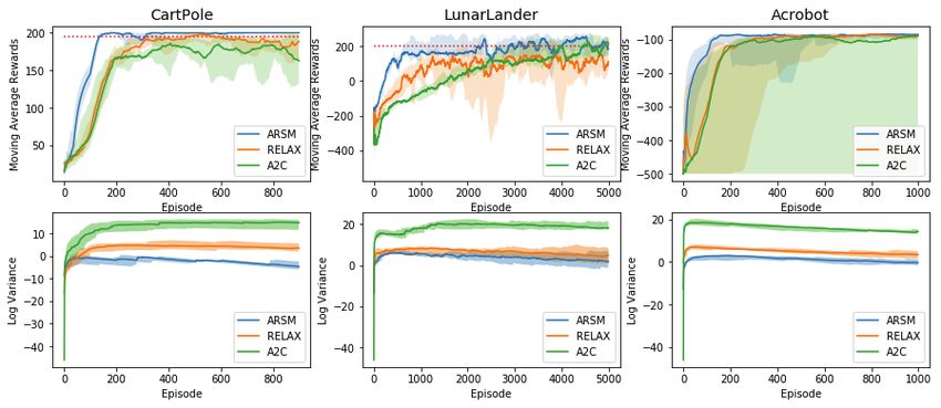
Figure 3. Top row: Moving average reward curves. Bottom row: Log-variance of gradient estimator. In each plot, the solid lines are
the median value of ten independent runs (ten different random seeds for random initializations). The opaque bars are 10th and 90th
percentiles. Dashed straight lines in Cart Pole and Lunar Lander represent task-completion criteria.
both the true trajectory and all state-pseudo-action rollouts. rithm 3 and the provided code for more details. Using our
The results for RELAX and A2C are obtained by running current implementation that has not been optimized to fully
the code provided by Grathwohl et al. (2018)3 . take the advantage of parallel computing, to finish the num-
ber of episodes as in Figure 3, ARSM on average takes
We apply the ARSM policy gradient to three representative
677, 425, and 19050 seconds for CartPole, Acrobot, and
RL tasks with discrete actions, including the Cart Pole, Ac-
LunarLander, respectively. For comparison, for these three
robot, and Lunar Lander environments provided by OpenAI
tasks, RELAX on average takes 139, 172, and 3493 seconds
Gym (Brockman et al., 2016), and compare it with advan-
and A2C on average takes 92, 120, and 2708 seconds.
tage actor-critic algorithm (A2C) (Sutton et al., 2000) and
RELAX (Grathwohl et al., 2018). We report the moving-
average rewards and the estimated log-variance of the gradi- 5. Conclusion
ent estimator at every episode; for each episode, the reward
To backpropagate the gradients through categorical stochas-
score is obtained by running the updated policy on a new
tic layers, we propose the augment-REINFORCE-swap-
random environment; and the variance is obtained by first
merge (ARSM) estimator that is unbiased and exhibits low
applying exponential moving averages to the first and sec-
variance. The performance of ARSM is almost identical to
ond moments of each neural network parameter with decay
that of the true gradient when used for optimization involv-
0.99, and then taking the average of the estimated variances
ing a C-way categorical variable, even when C is very large
of all neural network parameters.
(such as C = 10, 000). For multiple C-way categorical
Shown in Figure 3 are the mean rewards over the last 100 variables organized into a single stochastic layer, multiple
steps; the opaque bar indicates 10th and 90th percentiles stochastic layers, or a sequential setting, the ARSM estima-
obtained by ten independent runs for each method (using tor clearly outperforms state-of-the-art methods, as shown
10 different random seeds for random initializations); the in our experimental results for both categorical latent vari-
solid line is the median value of these ten independent runs. able models and discrete-action policy optimization. We
ARSM outperform both baselines in all three tasks in terms attribute the outstanding performance of ARSM to both
of stability, moving average rewards, and log-variance of its unbiasedness and its ability to control variance by sim-
gradient estimator. All methods are cross validated by opti- ply combing its reward function with randomly generated
mizers {Adam Optimizer, RMSProp Optimizer} and learn- pseudo actions, where the number of unique pseudo actions
ing rates {1, 3, 10, 30} × 10−3 . Both the policy and critic is positively related to the uncertainties of categorical dis-
networks for A2C and RELAX have two 10-unit hidden lay- tributions and hence negatively correlated to how well the
ers with ReLU activation functions (Nair & Hinton, 2010). optimization algorithm has converged; there is no more need
The discount factor γ is 0.99 and entropy term is 0.01. The to construct separate baselines and estimate their parameters,
policy network of ARSM is the same as that of A2C and which also help make the optimization more robust. Some
RELAX, and the maximum number of allowed state-pseudo- natural extensions of the proposed ARSM estimator include
action rollouts of ARSM is set as 16, 64, and 1024 for Cart applying it to reinforcement learning with high-dimensional
Pole, Acrobot, and Lunar Lander, respectively; see Algo- discrete-action spaces or multiple discrete-action agents,
3
and various tasks in natural language processing such as
https://github.com/wgrathwohl/BackpropThroughTheVoidRL
sentence generation and machine translation.ARSM: Augment-REINFORCE-Swap-Merge Gradient for Categorical Variables
Acknowledgements Kingma, D. P. and Ba, J. Adam: A method for stochastic
optimization. arXiv preprint arXiv:1412.6980, 2014.
This research was supported in part by Award IIS-1812699
from the U.S. National Science Foundation and the Mc- Kingma, D. P. and Welling, M. Auto-encoding variational
Combs Research Excellence Grant. The authors acknowl- Bayes. arXiv preprint arXiv:1312.6114, 2013.
edge the support of NVIDIA Corporation with the donation
of the Titan Xp GPU used for this research, and the compu- Kucukelbir, A., Tran, D., Ranganath, R., Gelman, A., and
tational support of Texas Advanced Computing Center. Blei, D. M. Automatic differentiation variational infer-
ence. Journal of Machine Learning Research, 18(14):
References 1–45, 2017.
Andriyash, E., Vahdat, A., and Macready, B. Improved Liu, H., Feng, Y., Mao, Y., Zhou, D., Peng, J., and Liu, Q.
gradient-based optimization over discrete distributions. Action-dependent control variates for policy optimization
arXiv preprint arXiv:1810.00116, 2018. via Stein identity. In ICLR, 2018.
Bengio, Y., Léonard, N., and Courville, A. Estimating or Maas, A. L., Hannun, A. Y., and Ng, A. Y. Rectifier non-
propagating gradients through stochastic neurons for con- linearities improve neural network acoustic models. In
ditional computation. arXiv preprint arXiv:1308.3432, ICML, 2013.
2013.
Maddison, C. J., Mnih, A., and Teh, Y. W. The Concrete
Brockman, G., Cheung, V., Pettersson, L., Schneider, J., distribution: A continuous relaxation of discrete random
Schulman, J., Tang, J., and Zaremba, W. OpenAI Gym. variables. In ICLR, 2017.
arXiv preprint arXiv:1606.01540, 2016.
McFadden, D. Conditional Logit Analysis of Qualitative
Casella, G. and Robert, C. P. Rao-Blackwellisation of sam- Choice Behavior. In Zarembka, P. (ed.), Frontiers in
pling schemes. Biometrika, 83(1):81–94, 1996. Econometrics, pp. 105–142. Academic Press, New York,
1974.
Cheng, P., Liu, C., Li, C., Shen, D., Henao, R., and Carin,
L. Straight-through estimator as projected Wasserstein Mnih, A. and Gregor, K. Neural variational inference and
gradient flow. In NeurIPS 2018 Bayesian Deep Learning learning in belief networks. In ICML, pp. 1791–1799,
Workshop, 2018. 2014.
Grathwohl, W., Choi, D., Wu, Y., Roeder, G., and Duve- Mnih, A. and Rezende, D. J. Variational inference for Monte
naud, D. Backpropagation through the Void: Optimizing Carlo objectives. arXiv preprint arXiv:1602.06725, 2016.
control variates for black-box gradient estimation. In
ICLR, 2018. Mnih, V., Badia, A. P., Mirza, M., Graves, A., Lillicrap,
T., Harley, T., Silver, D., and Kavukcuoglu, K. Asyn-
Greensmith, E., Bartlett, P. L., and Baxter, J. Variance reduc-
chronous methods for deep reinforcement learning. In
tion techniques for gradient estimates in reinforcement
ICML, pp. 1928–1937, 2016.
learning. J. Mach. Learn. Res., 5(Nov):1471–1530, 2004.
Gregor, K., Danihelka, I., Mnih, A., Blundell, C., and Wier- Naesseth, C., Ruiz, F., Linderman, S., and Blei, D. Reparam-
stra, D. Deep autoregressive networks. In ICML, pp. eterization gradients through acceptance-rejection sam-
1242–1250, 2014. pling algorithms. In AISTATS, pp. 489–498, 2017.
Gu, S., Levine, S., Sutskever, I., and Mnih, A. MuProp: Nair, V. and Hinton, G. E. Rectified linear units improve
Unbiased backpropagation for stochastic neural networks. restricted Boltzmann machines. In ICML, pp. 807–814,
In ICLR, 2016. 2010.
Gu, S., Lillicrap, T., Ghahramani, Z., Turner, R. E., and Owen, A. B. Monte Carlo Theory, Methods and Examples,
Levine, S. Q-Prop: Sample-efficient policy gradient with chapter 8 Variance Reduction. 2013.
an off-policy critic. In ICLR, 2017.
Paisley, J., Blei, D. M., and Jordan, M. I. Variational
Hinton, G. Neural networks for machine learning coursera Bayesian inference with stochastic search. In ICML, pp.
video lectures - Geoffrey Hinton. 2012. 1363–1370, 2012.
Jang, E., Gu, S., and Poole, B. Categorical reparameteriza- Peters, J. and Schaal, S. Natural actor-critic. Neurocomput-
tion with Gumbel-softmax. In ICLR, 2017. ing, 71(7-9):1180–1190, 2008.ARSM: Augment-REINFORCE-Swap-Merge Gradient for Categorical Variables
Raiko, T., Berglund, M., Alain, G., and Dinh, L. Tech- Weaver, L. and Tao, N. The optimal reward baseline for
niques for learning binary stochastic feedforward neural gradient-based reinforcement learning. In UAI, pp. 538–
networks. arXiv preprint arXiv:1406.2989, 2014. 545, 2001.
Ranganath, R., Gerrish, S., and Blei, D. Black box varia- Williams, R. J. Simple statistical gradient-following al-
tional inference. In AISTATS, pp. 814–822, 2014. gorithms for connectionist reinforcement learning. In
Reinforcement Learning, pp. 5–32. Springer, 1992.
Rezende, D. J., Mohamed, S., and Wierstra, D. Stochas-
tic backpropagation and approximate inference in deep Wu, C., Rajeswaran, A., Duan, Y., Kumar, V., Bayen, A. M.,
generative models. In ICML, pp. 1278–1286, 2014. Kakade, S., Mordatch, I., and Abbeel, P. Variance reduc-
tion for policy gradient with action-dependent factorized
Ross, S. M. Introduction to Probability Models. Academic baselines. In ICLR, 2018.
Press, 10th edition, 2006.
Yin, M. and Zhou, M. ARM: Augment-REINFORCE-
Ruiz, F. J. R., Titsias, M. K., and Blei, D. M. The general- merge gradient for stochastic binary networks. In ICLR,
ized reparameterization gradient. In NIPS, pp. 460–468, 2019.
2016.
Zhang, Q. and Zhou, M. Nonparametric Bayesian Lomax
Schulman, J., Levine, S., Abbeel, P., Jordan, M., and Moritz, delegate racing for survival analysis with competing risks.
P. Trust region policy optimization. In ICML, pp. 1889– In NeurIPS, pp. 5002–5013, 2018.
1897, 2015. Zhou, M. Beta-negative binomial process and exchangeable
random partitions for mixed-membership modeling. In
Sutton, R. S. and Barto, A. G. Reinforcement Learning: An
NIPS, pp. 3455–3463, 2014.
Introduction. 1998.
Zhou, M. and Carin, L. Negative binomial process count
Sutton, R. S., McAllester, D. A., Singh, S. P., and Mansour, and mixture modeling. arXiv preprint arXiv:1209.3442v1,
Y. Policy gradient methods for reinforcement learning 2012.
with function approximation. In NIPS, pp. 1057–1063,
2000.
Tanner, M. A. and Wong, W. H. The calculation of poste-
rior distributions by data augmentation. J. Amer. Statist.
Assoc., 82(398):528–540, 1987.
Titsias, M. K. and Lázaro-Gredilla, M. Local expectation
gradients for black box variational inference. In NIPS,
pp. 2638–2646, 2015.
Train, K. E. Discrete Choice Methods with Simulation.
Cambridge University Press, 2nd edition, 2009.
Tucker, G., Mnih, A., Maddison, C. J., Lawson, J., and Sohl-
Dickstein, J. REBAR: Low-variance, unbiased gradient
estimates for discrete latent variable models. In NIPS, pp.
2624–2633, 2017.
Tucker, G., Bhupatiraju, S., Gu, S., Turner, R., Ghahramani,
Z., and Levine, S. The mirage of action-dependent base-
lines in reinforcement learning. In ICML, pp. 5015–5024,
2018.
van den Oord, A., Vinyals, O., et al. Neural discrete repre-
sentation learning. In NIPS, pp. 6306–6315, 2017.
Van Dyk, D. A. and Meng, X.-L. The art of data augmenta-
tion. Journal of Computational and Graphical Statistics,
10(1):1–50, 2001.You can also read