DYETC: DYNAMIC ELECTRONIC TOLL COLLECTION FOR TRAFFIC CONGESTION ALLEVIATION

Page created by Calvin Kim
 
CONTINUE READING
DYETC: DYNAMIC ELECTRONIC TOLL COLLECTION FOR TRAFFIC CONGESTION ALLEVIATION
The Thirty-Second AAAI Conference
                                                        on Artificial Intelligence (AAAI-18)

                                DyETC: Dynamic Electronic Toll Collection
                                    for Traffic Congestion Alleviation
                         Haipeng Chen,1,† Bo An,1,† Guni Sharon,2,‡ Josiah P. Hanna,2,§ ,
                              Peter Stone,2,§ Chunyan Miao,1,† Yeng Chai Soh1,†
                                                   1
                                                     Nanyang Technological University
                                                      2
                                                        University of Texas at Austin
                                            †
                                                {chen0939,boan,ascymiao,ecsoh}@ntu.edu.sg
                                                         ‡
                                                           gunisharon@gmail.com
                                                    §
                                                      {jphanna,pstone}@cs.utexas.edu

                            Abstract                                         over time. However, these tolling schemes still assume that
                                                                             traffic demands are fixed and are known a priori, and thus are
  To alleviate traffic congestion in urban areas, electronic toll
                                                                             static in essence. In practice, traffic demands fluctuate and
  collection (ETC) systems are deployed all over the world.
  Despite the merits, tolls are usually pre-determined and fixed              cannot be predicted accurately, especially when the traffic is
  from day to day, which fail to consider traffic dynamics and                abnormal (e.g., in case of traffic accidents, or city events).
  thus have limited regulation effect when traffic conditions are             As a result, these static tolling schemes usually have limited
  abnormal. In this paper, we propose a novel dynamic ETC                    regulation effect. One recent work of Sharon et al. (2017)
  (DyETC) scheme which adjusts tolls to traffic conditions in                 proposes a dynamic tolling scheme called Δ-tolling, which
  realtime. The DyETC problem is formulated as a Markov                      assigns a toll to each road proportional to the difference be-
  decision process (MDP), the solution of which is very chal-                tween its current travel time and its free-flow travel time.
  lenging due to its 1) multi-dimensional state space, 2) multi-             However, Δ-tolling does not take a proactive approach to-
  dimensional, continuous and bounded action space, and 3)                   wards changes in the demand side. Instead, D-tolling only
  time-dependent state and action values. Due to the complex-
                                                                             reacts to such changes once they are detected. In contrast,
  ity of the formulated MDP, existing methods cannot be ap-
  plied to our problem. Therefore, we develop a novel algo-                  we propose a novel dynamic tolling scheme which optimizes
  rithm, PG-β, which makes three improvements to traditional                 traffic over the long run, with the following three major con-
  policy gradient method by proposing 1) time-dependent value                tributions.
  and policy functions, 2) Beta distribution policy function and                The first key contribution of this paper is a formal model
  3) state abstraction. Experimental results show that, com-                 of the DyETC problem. Since MDPs have various advan-
  pared with existing ETC schemes, DyETC increases traffic
  volume by around 8%, and reduces travel time by around
                                                                             tages in modelling long term planning problems with uncer-
  14.6% during rush hour. Considering the total traffic volume                tainty, we formulate the DyETC problem as a discrete-time
  in a traffic network, this contributes to a substantial increase            MDP. Though several existing methods have been proposed
  to social welfare.                                                         to solve the traffic assignment problem with MDP (Aka-
                                                                             matsu 1996; Baillon and Cominetti 2008), our method is
                                                                             notably distinct from these works, in the sense that they con-
                        Introduction                                         sider the uncertainty of drivers’ route choice behavior, while
Nowadays, governments face a worsening problem of traf-                      this work considers the uncertainty of traffic demand as well.
fic congestion in urban areas. To alleviate road conges-                      The state of the formulated MDP is the number of vehicles
tion, a number of approaches have been proposed, among                       on a road that are heading to certain destination, the action
which ETC has been reported to be effective in many coun-                    is the toll on each road, and the formulated MDP has 1) a
tries and areas (e.g., Singapore (LTA 2017), Norway (Au-                     multi-dimensional state space, 2) multi-dimensional, contin-
toPASS 2017)). The tolls of different roads and time pe-                     uous and bounded action space, and 3) time dependent state
riods are different, so that the vehicles are indirectly reg-                and action values.
ulated to travel through less congested roads with lower
                                                                                Due to the huge size of the MDP, it is very challenging
tolls. However, although current ETC schemes vary tolls
                                                                             to find its optimal policy. Traditional reinforcement learning
at different time periods throughout a day, they are pre-
                                                                             algorithms based on tabular representations of the value and
determined and fixed at the same periods from day to day. A
                                                                             policy functions (e.g., tabular Q-learning (Watkins 1989),
few dynamic road pricing schemes (Joksimovic et al. 2005;
                                                                             prioritized sweeping (Moore and Atkeson 1993), Monte
Lu, Mahmassani, and Zhou 2008; Zhang, Mahmassani, and
                                                                             Carlo Tree Search (MCTS) (Coulom 2006) and UCT (UCB
Lu 2013) have been proposed in the transportation research
                                                                             applied to trees) (Kocsis and Szepesvári 2006)) cannot be
community which consider the variations of traffic demands
                                                                             applied to our problem due to the large scale state and ac-
Copyright  c 2018, Association for the Advancement of Artificial             tion spaces. Value-based methods with function approxima-
Intelligence (www.aaai.org). All rights reserved.                            tion (Precup, Sutton, and Dasgupta 2001; Maei et al. 2010;

                                                                       757
DYETC: DYNAMIC ELECTRONIC TOLL COLLECTION FOR TRAFFIC CONGESTION ALLEVIATION
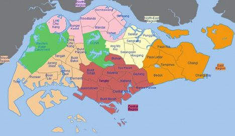
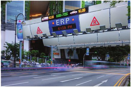
Nichols and Dracopoulos 2014; Mnih et al. 2015), which                 gapore to alleviate its traffic congestion, especially in the
represent the state-action values (often referred to as “Q-            central region (Figure 1(a)). In an ETC system, vehicles are
values”) with function approximators are also inefficient due           charged when they pass through ETC gantries (Figure 1(b))
to the complexity in selecting the optimal action in a contin-         and use priced roads during peak hours. Typically, ETC rates
uous action space. While policy gradient methods (Williams             vary from different roads and time periods, which encour-
1992; Sutton et al. 1999; Peters and Schaal 2008; Schul-               ages vehicles to change their travel routes in order to alle-
man et al. 2015) work well in solving large scale MDPs with            viate traffic congestion. As shown in Figure 1(c), while an
continuous action space, current policy gradient approaches            ETC gantry charges different ETC rates at different time pe-
usually focus on MDPs with unbounded action space. To                  riods, the rates are fixed during certain time periods from
handle bounded action spaces, Hausknecht and Stone (2016)              Monday to Friday. This framework, which is demonstrated
propose three approaches (i.e., zeroing, squashing and in-             to have significantly improved Singapore’s traffic, still has
verting) on the gradients which force the parameters to pre-           two major shortcomings. First, the current ETC system is
serve in their intended ranges. These manually enforced con-           determined based on the historical traffic flows, which fails
straints may deteriorate the solution’s optimality.                    to adjust to the uncertainty of traffic demand. In reality, the
   To solve the DyETC problem, we make our second key                  real-time traffic demand could fluctuate. For example, dur-
contribution by proposing an efficient solution algorithm,              ing morning rush hour, we may know the average traffic de-
PG-β (Policy Gradient method with Beta distribution based              mand based on history, but the exact demand cannot be pre-
policy functions). In the DyETC problem, the value of a state          cisely predicted. As a result, if we set tolls merely accord-
is time-dependent. We make our first improvement by ex-                 ing to average traffic demand but the real demand is not as
tending the formulated MDP as time-dependent, adapting                 severe as expected, few vehicles will go through this road
the traditional policy gradient method to maintain a sepa-             even if the congestion is not severe since they are scared off
rate value and policy function for each time period, and de-           by the high tolls. Under such cases, the current ETC sys-
rive the update rule for the parameters. Moreover, to bal-             tem will have less positive or even negative effect on the
ance the tradeoff between “exploration” and “exploitation”             traffic condition. Second, current ETC rating systems fail to
for continuous action space, traditional methods either per-           precisely respond to the extent to which the traffic is con-
form poorly in unbounded action space MDPs (Sutton et                  gested. As we can see from Figure 1(c), the interval of the
al. 1999), or manually enforce the parameters to guarantee             current tolling scheme is 0.5. For example, the tolls are ei-
the bounded action space (Hausknecht and Stone 2016). To               ther 0 or 0.5, while the optimal toll might be somewhere
overcome this deficiency, we make the second improvement                between these two rates. In such cases, the current tolling
by proposing a novel form of policy function, which is based           scheme can hardly reveal and react to the accurate conges-
on the Beta probability distribution, and deriving its corre-          tion level. To further alleviate traffic congestion in urban ar-
sponding update rules. Last, to further improve scalability            eas, we propose a novel dynamic ETC scheme which is 1)
of PG-β, we exploit the structure of the formulated DyETC              fully dynamic and 2) finer-grained.1
problem, and propose an abstraction over the state space,
which significantly reduces the scale of the state space,                      Formulation of the DyETC Problem
while maintaining near-optimality.
   Third, we conduct extensive experimental evaluations to             In this section, we first introduce the dynamic ETC system,
compare our proposed method with existing policy gradi-                and then formulate the DyETC problem as an MDP.
ent methods as well as current tolling schemes. The results
demonstrate that PG-β performs significantly better than                Dynamic ETC System
state-of-the-art policy gradient methods and current tolling           The urban city area can be abstracted as a directed road net-
schemes. Performed in a road network of Singapore Central              work G = (E, Z, O), where E is the set of roads, Z is the
Region, DyETC increases the traffic volume by around 8%,                set of zones and O is the set of origin-destination (OD) pairs.
and reduces the total travel time by around 14.6%.                     Take Singapore Central Region as an example (Figure 2),
                                                                       there are altogether 11 zones and 40 abstracted roads.2 The
                 Motivation Scenario                                   decision time horizon H (usually the length of rush hour) is
                                                                       discretized into several intervals, with a length of τ (e.g., 10
                                                                       minutes) for each interval. For time period t = 0, 1, . . . , H,
                                                                           1
                                                                             Such dynamic toll information can be displayed on telescreens
                                                                       along roads which can be easily accessed by drivers. Moreover,
                                                                       with the introduction of intelligent agent-based vehicles and even
                                                                       autonomous vehicles (e.g., in Singapore (LTA 2016)), autonomous
                                                                       agents are able to aid the drivers in deciding the optimal travel
   (a) ETC system      (b) ETC gantry        (c) ETC rates             routes under the proposed DyETC scheme.
                                                                           2
                                                                             Each pair of two adjacent zones has two directed roads. If there
                Figure 1: ETC in Singapore                             are multiple roads from one zone to another, they could be treated
                                                                       as one abstracted road, where the capacity of the abstracted road
                                                                       is a sum of these roads, and the length of the abstracted road is an
  Since 1998, an ETC system has been deployed in Sin-                  average of these roads.

                                                                 758
DYETC: DYNAMIC ELECTRONIC TOLL COLLECTION FOR TRAFFIC CONGESTION ALLEVIATION
Bukit Timah
                                                                        Bishan
                                                                                                               ܵ௘௧                                            ܵ௘௧ାଵ 
                                                                                    Toa Payoh

                                                            Novena

                                                                          Kallang           Geylang

                                                                                                                                                    ‫ݐ‬                                            ‫ ݐ‬൅ ͳ
                                                                                                                                     ௧
                                                      Tanglin                                                                       ܵ௘ǡ௜௡                            ௧ାଵ
                                                                                                                                                                                       ܵ௘ǡ௜௡       
                                                                       Central Area                                                  ௧
                                                                                                                                    ܵ௘ǡ௢௨௧                             ௧ାଵ
                                                                                                                                                                                       ܵ௘ǡ௢௨௧        
                                     Queenstown
                                                                                                                –                                         – ൅ ͳ
                                                                                    Marine Parade                                                           
                                                                Bukit Merah
                                                                                                                                                –                                  – ൅ ͳ  

  (a) Singapore Central Region         (b) Abstracted road network
                                                                                                               Figure 3: Event timeline of two subsequent time periods
      Figure 2: Road network of Singapore Central Region
                                                                                                            cost, and the aggregate choice of all the vehicles is assumed
                                              t                                                             to follow the discrete choice model in Eq.(3). We formulate
we denote an OD pair as a tuple zi , zj , qi,j , Pi,j , where
                                                    t                                                       the DyETC problem as a discrete time MDP, due to its ad-
zone zi is the origin, zone zj is the destination, qi,j denotes                                             vantages in modeling sequential planning problems.
traffic demand during time t, and Pi,j denotes the set of all                                                State & action. At the beginning of time period t, the state
possible paths from zi to zj which do not contain a cycle.                                                  is defined as the number of vehicles ste,j on each road e that
Different from most previous works which assume that the
                     t                                                                                      are going to destination zj . ste = ste,j  is the state vector
OD traffic demand qi,j   for a certain time period t is fixed and
known a priori, we consider dynamic OD travel demand,                                                       of a road e, and st = ste  is the state matrix of the road
where the travel demand of an OD pair follows a probability                                                 network G. At time t, the government’s action is to set the
                               t
distribution function (PDF) qi,j         t
                                  ∼ f (qi,j ).                                                              tolls at = ate , e ∈ E  , where E  ⊆ E is the subset of roads
   We follow the commonly used travel time model (BPR                                                       which have ETC gantries.
1964) to define the travel time on a road e at t:                                                                Since both the traffic condition and tolls change over time,
                                                                                                            a vehicle has an incentive to change its path once it reaches
                   Tet = Te0 [1 + A(ste /Ce )B ].                                               (1)         the end of a road. The path readjustment does not depend
ste is the number of vehicles on road e. Ce and          are road-       Te0                                on the past decisions of the vehicle, but only depends on its
specific constants, where Te0 is interpreted as the free-flow                                                 destination. Therefore, for a vehicle that arrives at the end
travel time, and Ce is the capacity of the road. A and B                                                    zi of a road e, we treat it as a vehicle from the new origin
are constants which quantify the extent to which congestion                                                 zi , while maintaining its destination zj . To distinguish these
influences travel time. Consequently, average travel speed is                                                vehicles with those that really use zi as the origin, we define:
Le              Le                                                                                                                                                          t
Tet = Te0 [1+A(ste /Ce )B ] , where Le is the length of road e. At
                                                                                                            Definition 1. At time period t, the primary OD demand qi,j
time t, the travel cost of a path p ∈ Pi,j , which we denote as                                             from zi to zj is the number of vehicles that originate from zi
                                                                                                                                                                     t
ci,j,p , consists of both time and monetary costs:                                                          at time period t; while the secondary OD demand q̄i,j       is the
                                                                                                           number of vehicles that come from zi ’s neighbouring roads
                   cti,j,p =        (ate + ωTet ),             (2)                                          during time period t − 1 that are heading for destination zj .
                                 e∈p
                                                                                                                We refer to Figure 3 as an illustration of the event timeline
where    ate is the toll imposed on road e, and ω is a con-                                                 for two subsequent time periods. At the beginning of time
stant which reveals the value of time. To make the analysis                                                 period t, tolls are decided based on the state st of the current
tractable, we assume that all vehicles have the same value                                                  time period. After the tolls are announced to the vehicles,
of time. Given the current traffic condition (i.e., number of                                                the vehicles will react to the tolls and traffic conditions and
vehicles on each road) and tolls, each vehicle will select a                                                a SUE will gradually form during time period t. In practice,
path p ∈ Pi,j leading to its destination, which aggregately                                                 it usually takes time to form an SUE and it keeps evolving
forms a traffic equilibrium. To describe this traffic equilib-                                                over time. Before the SUE is formed, the number of vehi-
rium, we adopt a widely-used stochastic user equilibrium                                                    cles on a road is normally larger (or smaller) than that in
(SUE) model (Lo and Szeto 2002; Lo, Yip, and Wan 2003;                                                      the SUE, while after the SUE, the number is usually smaller
Huang and Li 2007), where the portion of traffic demand                                                      (or larger). To make the analysis tractable, we use the num-
xti,j,p travelling with path p ∈ Pi,j is                                                                    ber of vehicles when the SUE is formed to approximate the
                                                                                                            average number of vehicles on a road during time period t.
                                 exp{−ω  cti,j,p }                                                         State transition. After the SUE is formed, the state of the
               xti,j,p =                        t
                                                       .                                        (3)
                             p ∈Pi,j exp{−ω ci,j,p }
                                                                                                            next time period can be derived. At the beginning of time
                                                                                                            t + 1, the number of vehicles on road e is determined by the
ω  is a constant measuring vehicles’ sensitivity to travel cost.                                           number of vehicles that 1) stay on road e, 2) exit road e, and
                                                                                                            3) enter road e during time t. Formally,
An MDP Formulation
                                                                                                                                         st+1    t      t          t
                                                                                                                                          e,j = se,j − se,j,out + se,j,in .                                                          (4)
In general, the government sets the tolls for the current time
period and announces them to the vehicles, while each ve-                                                   We make a mild and intuitive assumption that the number
hicle individually selects paths according to the total travel                                              of vehicles ste,j,out that exit a road e is proportional to the

                                                                                                      759
average travel speed during time period t. Thus,                                                     Solution Algorithm: PG-β
                                                                                      It is very challenging to find the optimal policy function
                                υt · τ          ste,j τ                               for the formulated DyETC problem due to three reasons.
       ste,j,out   =   ste,j   · e     = 0                     ,          (5)
                                 Le     Te [1 + A(ste /Ce )B ]                        First, the state space is multi-dimensional w.r.t. the number
                                                                                      of roads and destinations. Second, the action space is also
where Le is the length of road e.                                                     multi-dimensional w.r.t. the number of ETC gantries. More-
   We now derive the last term ste,j,in in Eq.(4). Recall that                        over, the action space is bounded and continuous. Last, both
the total demand of an OD pair is the sum of primary and                              the state and action values are dependent on the specific time
secondary OD demand. The secondary demand of an OD                                    periods. As a result, it is intractable to find the optimal pol-
pair from zi to zj is                                                                 icy function by simply going through all combinations of
                                                                                     state-action pairs, which would be on an astronomical order.
                    t
                  q̄i,j =    +
                                   ste ,j,out ,           (6)                           Although numerous reinforcement learning algorithms
                                     e      =zi                                       have been proposed to solve MDPs, they cannot be directly
                                                                                      applied to our problem due to the complexities presented
where e+ is the ending point of road e (correspondingly, we                           above. While the policy gradient methods (Williams 1992;
use e− to denote the starting point of e). Note that during                           Sutton et al. 1999) have shown promise in solving large scale
time t, for an OD traffic demand from zi to zj to be counted                           MDPs with continuous action spaces, current policy gradi-
as a component of ste,j,in , two conditions must be satisfied.                         ent methods usually focus on MDPs with unbounded action
First, zi should be the starting point of e, i.e., zi = e− . Sec-                     spaces. In the following, we present our solution algorithm,
ond, at least one of the paths from zi to zj should contain                           PG-β (Policy Gradient method with Beta distribution based
road e, i.e., e ∈ p ∈ Pi,j . Thus, we have:                                           and time-dependent policy functions), with novel improve-
                                                                                     ments to typical applications of policy gradient methods.
       ste,j,in =        −
                                       t
                                     (qi,j     t
                                           + q̄i,j ) · xti,j,p . (7)
                          zi =e ∩e∈p∈Pi,j
                                                                                      General Framework of PG-β
Combining Eqs.(4)-(7), there is:
                                                                                        Algorithm 1: PG-β
                             ste,j τ                                                                 t           t
                                                                                       1 Initialize ϑ ← ϑ 0 , θ ← θ 0 , ∀t = 0, 1, . . . , H;
 st+1    t
  e,j = se,j       − 0                     +
                    Te [1 + A(ste /Ce )B ]                          (8)                2 repeat
                                  
                           t
                         (qi,j +             t              t
                                            se ,j,out ) · xi,j,p .                    3    Generate an episode s0 , a0 , R0 , . . . , sH , aH , RH ;
       zi =e− ∩e∈p∈Pi,j              +      e    =vi                                  4    for t = 0, . . . , H do
                                                                                                       H
                                                                                       5       Qt ← t =t Rτ ;
Value function & Policy. From the perspective of the gov-
                                                                                       6       δ ← Qt − v̂(st , at , ϑ t )
ernment, a good traffic condition means that, during the
planning time horizon H, the total traffic volume (i.e., the                            7       ϑ t ← ϑ t + βδ∇ϑ t v̂(st , ϑ t );
number of vehicles that reach their destinations) is maxi-                             8       θ t ← θ t + β  δ∇θ t log π t (at |st , θ t )
mized.3 Formally, we define the immediate reward function                               9 until #episodes= M
                                                                                                   t
Rt (st , at ) as the number of vehicles that arrive at their des-                     10 return θ , ∀t = 0, 1, . . . , H;
tinations during time t:
                                                    ste,j τ                              The idea of PG-β is to approximate the policy function
    Rt (st ) =                                                       .    (9)         with a parameterized function, and update the parameter
                       e∈E         zj =e+    Te0 [1 + A(ste /Ce )B ]                  with stochastic gradient descent method. More specifically,
                                                                                      PG-β incorporates an actor-critic architecture, where the
Note that we simplify the notation as Rt (st ) since it does                          “actor” is the learned policy function which performs action
not depend on at . The long term value function v t (st ) is the                      selection, and the “critic” refers to the learned value function
sum of rewards from t to t + H:                                                       measuring the performance of the current policy function.
                                 t+H                     
                                                                                           In Algorithm 1, the input of PG-β includes the plan-
                   v t (st ) =              γ t −t Rt (st ),             (10)         ning horizon H, the state transition function Eq.(8), a set
                                    t =t
                                                                                      of parameterized value functions v t (s, ϑ t ) w.r.t. parameter
where γ is a discount factor. At time t, a policy π t (at |st ) is                    ϑ t (∀t = 0, . . . , H), and a set of parameterized policy func-
a function which specifies the conditional probability of tak-                         tions π t (a|s, θ t ) w.r.t. parameter θ t (∀t = 0, . . . , H). The al-
ing an action at , given a certain state st . The optimal policy                      gorithm starts with an initialization of the parameters ϑ t and
maximizes the value function in Eq.(10):                                              θ t . It then enters the repeat loop (Lines 2-9). In the repeat
                                                                                      loop, it first simulates an episode, which contains a series of
                   π t,∗ (at |st ) = arg maxπt v t (st ).                (11)         state-action pairs in the planning horizon H. The states are
                                                                                      generated following the state transition function Eq.(8), the
   3
     DyETC can be extended to optimize other objective functions,                     actions are selected following the policy function π(a|s, θ ),
total travel time among them, by changing the reward function ap-                     while the immediate rewards are computed with Eq.(9). Af-
propriately. We leave such extensions to future work.                                 ter an episode is simulated, the algorithm then updates the

                                                                                760
parameters at each time period t = 0, . . . , H (Lines 4-                             For stochastic gradient, a sampled action At is used to re-
9) with stochastic gradient descent method. Qt denotes the                            place the expectation, i.e.,
sum of rewards from time t to H obtained from the sim-
                                                                                                                        ∇θ t π t (At |st , θ t )
ulated episode, which reveals the “real” value obtained by                                     ∇θ t v t (st ) = Qtπ (st , At )
the current policy, while v̂ t (st , ϑ t ) is the “estimated” sum of                                                     π t (At |st , θ t )
rewards approximated by the parameterized value function                                        = Q (s , A )∇θ t log π (At |st , θ t )
                                                                                                   t t    t           t

v t (st , ϑ t ). Consequently, δ denotes the difference of these
two terms. In Lines 7-8, PG-β updates the parameters by
our derived update rule which is to be introduced in the two                          A Novel Policy Function Based on the Beta PDF
subsequent subsections. This process iterates until the num-
ber of episodes reaches a pre-defined large number M (e.g.,                            An important challenge of the policy gradient method is to
100,000).                                                                             balance the “exploitation” of the optimal action generated
                                                                                      from the policy function and the “exploration” of the action
Policy Gradient for Time-Dependent MDP                                                space to ensure that the policy function is not biased. For
                                                                                      MDPs with continuous action space, a Normal PDF has been
A fundamental property of traditional MDPs is that the value                          used in recent works (Sutton and Barto 2011) as the policy
of a state does not change over time. However, such prop-                             function. While Normal PDF works well in cases where the
erty does not exist in our problem. Intuitively, with the same                        action space is unbounded, it is not suitable for MDPs which
number of vehicles on the road network, the number of ve-                             have bounded action spaces, since the action generated by
hicles that reach the destinations (i.e., the objective) still de-                    the Normal PDF policy function would possibly become in-
pends on the OD demand of a specific time period as well                               feasible. In practice, tolls are restricted within a certain inter-
as future periods. Consequently, the value of an action is                            val [0, amax ] (e.g., in Singapore, tolls are within 6 Singapore
also dependent on the specific time period. This class of                              dollars). A straightforward adaptation is to project the gener-
MDPs is called finite horizon MDPs (FHMDPs). For FH-                                   ated action to the feasible action space whenever it is infea-
MDPs, we need to maintain and update a value function                                 sible. However, experimental results (will be presented later
v t (s, ϑ t ) and a policy function π t (a|s, θ t ) for each time step                in Figure 4(a)) show that, even with such adaptation, Normal
t = 0, 1, . . . , H, as shown in Algorithm 1. The following                           PDF policy function performs poorly in solving MDPs with
theorem ensures that the update of θ t improves action selec-                         bounded action spaces.
tion in the FHMDP.4                                                                      To adapt policy gradient methods to bounded action
Theorem 1. The gradient function of policy gradient                                   space, we propose a new form of policy function, which is
method on FHMDPs is                                                                   derived from Beta PDF f (x):

       ∇θ t vπ (s) = Qt (st , at )∇θ t log π t (at |st , θ t ),          (12)                                      xλ−1 (1 − x)ξ−1
                                                                                                      f (x, λ, ν) =                ,         (13)
                                                                                                                       B(λ, ξ)
where Qt (st , at ) is the action value of at given state st .                                                               1
                                                                                      where the Beta function, B(λ, ξ) = 0 tλ−1 (1 − t)ξ−1 dt
Proof. We first write the state         value as the expected sum                     is a normalization constant, and the variable x ∈ [0, 1] is
of action values, i.e.,v t (st ) = at π t (at |st , θ t )Qt (st , at ),              bounded and continuous. For each road e, let xe = ae /amax ,
where Qt (st , at ) = st+1 P (st+1 , at , st )v t+1 (st+1 ). Since                    then the policy function is denoted as
both the transition probability function P (st+1 , at , st ) and                                                             xλe e −1 (1 − xe )ξe −1
the value function v t+1 (st+1 ) of time t + 1 do not depend                             πe (ae = xe amax |s, λe , ξe ) =                            ,         (14)
on θ t , Qt (st , at ) is also independent on θ t . Thus, we have                                                                   B(λe , ξe )
                                                                                     where λe = λe (φφ(s), θ λ ) and ξe = ξe (φ  φ(s), θ ξ ) are parame-
          ∇θ t v t (st ) =       t
                                   Qt (st , at )∇θ t π t (at |st , θ t )                                       λ         ξ
                                                                                      terized functions, and θ and θ are parameters to be approx-
                                    a
                                                  ∇θ t π t (at |st , θ t )           imated. For example, in the commonly utilized linear func-
          =            π (a |s , θ t )Qt (st , at )
                        t   t   t
                                                                                      tion approximation, each λe and ξe is represented by a linear
                  at                                     π t (st , at )               function of the parameters θ λ and θ ξ : λe = θ λ · φ (s), ξe =
          (multiplying and dividing by π t (at |st , θ t ))                           θ ξ · φ (s).
                             ∇θ t π t (at |st , θ t )                                 Proposition 1. Using Beta PDF policy function, the update
          = E[Qtπ (st , at )                          ].                                                      λ
                                                                                      rule for a parameter θe,e   ,j,i (associated with road e) is
                              π t (at |st , θ t )
                                                                                             λ           λ                                            ∂λe
                                                                                                  ,j,i←θe,e ,j,i +β δ[ln(xe )−Ψ(λe )+Ψ(λe +ξe )]
   4
     For FHMDPs, a natural alternative is to incorporate the time                           θe,e                                                       λ
                                                                                                                                                                  ,
                                                                                                                                                     ∂θe,e  ,j,i
as one extra dimension of state. However, experimental results (see
Figure 4(a)) show that this alternative does not work well using                          ξ           ξ                                                ∂ξe
                                                                                         θe,e  ,j,i←θe,e ,j,i +β δ[ln(1−xe )−Ψ(ξe )+Ψ(λe +ξe )]                   ,
polynomial basis functions where states are not interrelated. Other                                                                                    ξ
                                                                                                                                                     ∂θe,e  ,j,i
alternatives might be to utilize an intrinsic basis function, or use
deep neural networks to represent the policy functions. However,                      where β  and β  are learning rates for θλ and θξ , respec-
such intrinsic functions are very hard to find (perhaps it does not                    tively, Ψ(·) is the diagamma function. e , j and i respectively
exist), while the time consumed in training an effective neural net-                  correspond to a road, a destination and a dimension in the
work is usually way longer than training linear policy functions.                     basis functions.

                                                                                761
        β         β                      
Proof. For ease of notation, we discard the superscript t. In                                                                      

Eq.(12), for edge e and dimension i of θ λ , by substituting                            


π(a|s, θ ) with Eq.(14), we have                                                        


                                             λ                                                                                              
  ∂v(s)         Q(s, a)∂πe (ae |s, θe,e          ,j,i )                                                                                 

    λ
             =                 λ              λ
                                                                                                                                          
 ∂θe,e ,j,i     πe (ae |s, θe,e ,j,i )∂θe,e ,j,i                                      


                                                                                                                         β    β                
                                              λ
           Q(s, a)            ∂πe (ae |s, θe,e     ,j,i )   ∂λe
 =               λ                                           λ
                                                                                                   (a) Learning curve                             (b) Per episode runtime
     πe (ae |s, θe,e ,j,i )           ∂λe                 ∂θe,e  ,j,i

                                              λe −1
           Q(s, a)              ∂ξe         xe         ln xe (1 − xe )ξe −1            Figure 4: Performance of different policy gradient methods
 =               λ               ξ
                                          [                                 −
     πe (ae |s, θe,e  ,j,i ) ∂θ
                                e,e ,j,i
                                                         B(λe , ξe )
 xeλe −1 (1 − xe )ξe −1 ∂B(λe , ξe )/∂λe                                               Evaluation on Synthetic Data
                                                     ]
                B 2 (λe , ξe )                                                         We first conduct experiments on synthetic data. For policy
        Q(s, a)             ∂ξe                                                        gradient methods, we first obtain the policy function with
 =             λ             ξ
   πe (ae |s, θe,e       )
                    ,j,i ∂θ
                            e,e ,j,i
                                                                                       offline training, and then use the trained policy to evaluate
                                                                                       their performance. Unless otherwise specified, the parame-
 xeλe −1 (1 − xe )ξe −1 [ln xe − Ψ(λe ) + Ψ(λe + ξe )]                                 ters of this subsection are set as follows.
                         B(λe , ξe )                                                      Learning-related parameters. The learning rates of the
                                               ∂ξe                                     value function and policy function are hand-tuned as 10−7
 = Q(s, a)[ln xe − Ψ(λe ) + Ψ(λe + ξe )] ξ                                             and 10−10 , respectively. The discount factor γ is set as 1,
                                             ∂θe,e ,j,i                               which assigns same weights to rewards of different time pe-
By replacing Q(s, a) with δ, we obtain the update rule for                             riods in the finite time horizon H. The number of episodes
 λ
θe,e                                                    ξ                              for training is 50,000 and the number of episodes for valida-
      ,j,i . Similarly, we derive the update rule for θe,e ,j,i .
                                                                                       tion is 10,000.
State Abstraction                                                                         Road network-related parameters. The number of zones
As discussed above, there are two corresponding parame-                                in the simulation is set as |Z| = 5, and all zones can be des-
       λ              ξ                                                               tinations, i.e., |Z  | = |Z|. The number of roads is set to 14,
ters θe,e  ,j,i and θe,e ,j,i for each edge e, each edge e , each
                                                                                       and all roads have ETC gantries, i.e., |E  | = |E| = 14. The
destination j and each dimension i in the basis functions.                             lengths of roads are randomized within [4, 10] km, which is
As a result, the total number of parameters in the policy                              the usual length range between zones of a city. Capacity of a
function is of order ∝ |E|2 |Z|Hd, where |E|, |Z|, H and                               road is set as 50 vehicles per kilometer per lane. This amount
d are respectively the number of edges, number of vertices                             is obtained from an empirical study of Singapore roads (Ol-
(destinations), length of time horizon and number of dimen-                                                                      T0
sions in the basis functions. In this case, when a road net-                           szewski 2000). Free flow travel speed Lee = 0.5 km/min.
work grows too large, it becomes rather time consuming for                             The parameters in the travel time model Eq.(1) is set as
PG-β to learn an effective tolling policy. Moreover, higher                            A = 0.15, B = 4 according to (BPR 1964).
dimension states may lead to over-fitting. To handle these                                 Demand-related parameters. OD demand is simulated as
two issues, we conjecture:                                                             a step function of time, where demand at time t = 0 is the
                                                                                       lowest, and gradually grows to peak demand in the mid-
Conjecture 1. The vehicles on a same edge that are going
                                                                                       dle of the planning time horizon, and decreases again to a
to different destinations have almost equal effects on tolls.
                                                                                       lower level. The peak demand for each OD pair is random-
   This conjecture means that, for the tolls on road e, the                            ized within [8, 12] vehicles per minute, which is a reason-
parameters (weights) associated to se ,j and se ,i are equal:                        able amount. The OD demand at t = 0 (which is usually the
              λ
             θe,e           λ               λ
                   ,j,i = θe,e ,j  ,i = θe,e ,i , ∀j, j
                                                            
                                                                          (15)         beginning of rush hour) is set as 60% of the peak demand.
                                                                                       Initial state is randomized within [0.5, 0.7] of the capacity of
              ξ                 ξ                    ξ                
             θe,e  ,j,i   =   θe,e  ,j  ,i   =   θe,e  ,i , ∀j, j     (16)         a road.
The supporting evidence of this conjecture will be shown                                  Toll-related parameters. Maximum toll amax = 6. This
through experimental evaluations.                                                      value is obtained from the current toll scheme in Singa-
                                                                                       pore. Planning horizon H = 6. Length of a time period
                  Experimental Evaluation                                              τ = 10 mins. Passenger cost-sensitivity level ω  = 0.5, and
                                                                                       value of time ω = 0.5. We will evaluate other values for these
In this section, we conduct experiments on both simulated                              two terms.
settings and a real-world road network in Singapore Cen-                               Comparison of different policy gradient methods.
tral Region to evaluate our proposed DyETC scheme and its
                                                                                          We compare the learning curve and solution quality of
solution algorithm PG-β. All algorithms are implemented
                                                                                       PG-β with the following policy gradient algorithms.
using Java, all computations are performed on a 64-bit ma-
chine with 16 GB RAM and a quad-core Intel i7-4770 3.4                                 1. PG-N: policy gradient (PG) with Normal distribution
GHz processor.                                                                            based policy function.

                                                                                 762
                                                                                                                                                                                                                                                      
            β                           Δ                               β                       Δ                        β                      Δ                  β                      Δ                       β                          Δ    


               (a) Initial state                                                   (b) Initial demand                                                 (c) Cost sensitivity                                     (d) Value of time                                           (e) Maximum price

                                     Figure 5: Traffic volume (in thousands) of existing tolling schemes under various traffic conditions
                                                                                                                                             
               β                   Δ                                  β                                                               β             Δ                        β             Δ                                   β                   Δ           


                                                                                 Δ                                                                                                                  


               (a) Initial state                                                   (b) Initial demand                                                 (c) Cost sensitivity                                     (d) Value of time                                           (e) Maximum price

                                   Figure 6: Total travel time (in thousands) of existing tolling schemes under various traffic conditions

2. PG-I: PG with time-independent policy function.                                                                                                                              OD demand ratio, and PG-β works well under different ini-
3. PG-time: PG-β where time is incorporated into state.                                                                                                                         tial state and OD demand scales. Similarly in Figures 5c-5d,
                                                                                                                                                                                with a higher cost-sensitivity level and value of time, the
4. PG-β-abs: PG-β with state abstraction.                                                                                                                                       traffic volume of all tolling schemes increases. According
 Figure 4(a) shows the learning curve of different policy                                                                                                                       to Eq.(3), this is intuitive in the sense that when the travel-
 gradient methods, where x-axis is the number of training                                                                                                                       ling cost of a congested road grows (faster than a less con-
 episodes, y-axis is the traffic volume (in thousands). It shows                                                                                                                 gested road), vehicles diverge towards less congested roads
 that PG-β and PG-β-abs converge faster (in terms of num-                                                                                                                       with less travelling cost. When these two parameters grow
 ber of training episodes) than other policy gradient methods,                                                                                                                  too large, the regulation effect of all tolling schemes be-
 and achieve higher traffic volume after 50, 000 episodes. It is                                                                                                                 comes saturated and traffic volume converges to a maximum
 worth mentioning that the classical policy gradient method                                                                                                                     amount. In this case, PG-β has a larger maximum limit than
 PG-N cannot learn an effective policy in our problem. More-                                                                                                                    other tolling schemes. Figure 5e shows that PG-β works well
 over, the learning curves of PG-β and PG-β-abs almost over-                                                                                                                    with different maximum toll amounts, and it works even bet-
 lap, which gives supporting evidence to Conjecture 1. Fig-                                                                                                                     ter when the maximum toll amount grows. In general, PG-β
 ure 4(b) presents per episode runtime (in milliseconds) of                                                                                                                     outperforms existing tolling schemes under all settings. It
 different policy gradient methods, where PG-β-abs has the                                                                                                                      is worth mentioning that, the state-of-the-art Δ-tolling ap-
 shortest per episode runtime. Combining the two figures,                                                                                                                        proach, which does not take a pro-active approach towards
 we conclude that PG-β-abs is the best approach in terms of                                                                                                                     changes in the demand side, does not work well in our set-
 both runtime efficiency and optimality. In the following, we                                                                                                                    ting.
 implement PG-β-abs to compare with other existing tolling                                                                                                                         To demonstrate that our DyETC framework can be
 schemes, while using PG-β to denote PG-β-abs for neatness                                                                                                                      adapted to other objectives, we also evaluate the total travel
of notation.                                                                                                                                                                    time of different tolling schemes under the above settings
Comparison of PG-β with existing tolling schemes under                                                                                                                          (Figure 6, where the y-axis is the total travel time). We can
different settings. We now compare PG-β with the follow-                                                                                                                        see that PG-β still significantly outperforms all the other
 ing baseline tolling schemes:                                                                                                                                                  tolling schemes (the less total travel time, the better).
1. Fix: fixed toll proportional to average OD demand.
2. DyState: dynamic toll proportional to the state scale.
                                                                                                                                                                                Evaluation on a Real-World Road Network of
                                                                                                                                                                                Singapore Central Region
3. Δ-toll (Sharon et al. 2017).
                                                                                                                                                                                In this subsection, we evaluate the performance of PG-β for
4. P0: no tolls.                                                                                                                                                                its regulation effect on the morning rush hour traffic of Sin-
    To compare tolling schemes under different settings, we                                                                                                                     gapore Central Region. The number of episodes for training
 vary the traffic parameter which under evaluation, and keep                                                                                                                     PG-β is 500, 000, and the learning rates for the value and
 all the other parameters as stated above. Figure 5 shows                                                                                                                       policy functions are fine-tuned as 10−8 and 10−12 , respec-
 the traffic volume obtained by different tolling schemes un-                                                                                                                    tively. Figure 7 shows the abstracted road network of Sin-
 der different settings, where the y-axis is the traffic vol-                                                                                                                    gapore Central Region, where the zones are labelled from
 ume, and the x-axis is the value of the parameter that is                                                                                                                      1 to 11. The numbers along the roads denote the travel dis-
 under evaluation. Figures 5a-5b show that, the traffic vol-                                                                                                                     tance of the adjacent zones, which is obtained from Google
 ume increases linearly w.r.t. the increasing initial state and                                                                                                                 Map. Since the OD demand is not revealed by Singapore

                                                                                                                                                                      763
                                                                 extensive experimental evaluations to compare our proposed
                                                                                                
                                                                                                                                                         method with existing tolling schemes. The results show that


                                                                                                                                                          on a real world traffic network in Singapore, PG-β increases
                                                                        
                                                                                                                                                          the traffic volume by around 8%, and reduces the travel time


                                                                                                                                                        by around 14.6% during rush hour.
                                                                                                                                                      Our DyETC scheme can be adapted to various dynamic
                                                            
                                                                                          
                                                                                                                                           network pricing domains such as the taxi system (Gan et al.
                                 
                                                                                                                                                        2013; Gan, An, and Miao 2015) and electric vehicle charg-
                                                                                              
                                                                                                                                                ing stations network (Xiong et al. 2015; 2016). While our
                                                                                                                                                 current work focused on a single domain with a relatively
                                                                                                                                                        small scale traffic network, we will extend DyETC to larger
                                                                                                                                                          scale networks. Potential approaches include stochastic op-
       Figure 7: Singapore Central Region road network                                                                                                    timization methods such as CMA-ES (Hansen 2006), con-
                                                                                                                                                          tinuous control variants of DQN (Mnih et al. 2015) such as
                                                                                                                                                   DDPG (Lillicrap et al. 2015) and NAF (Gu et al. 2016), par-
 
                                                                                                                                                      allel reinforcement learning such as A3C (Mnih et al. 2016)
 
                                                                                                                                                   and variance reduction gradient methods such as Averaged-
 
 
                                                                                                                                                      DQN (Anschel, Baram, and Shimkin 2017).


                                                                                                                                                                          Acknowledgments
                                                                                   
       β                                       Δ                               β                                 Δ            We would like to thank the anonymous reviewers for their
       (a) Total traffic volume                                                               (b) Total travel time                                        suggestions. This research is supported by the National Re-
                                                                                                                                                          search Foundation, Prime Ministers Office, Singapore under
                                                                                                                                                          its IDM Futures Funding Initiative. A portion of this work
Figure 8: Performance of existing tolling schemes evaluated                                                                                               has taken place in the Learning Agents Research Group
in Singapore Central Region                                                                                                                               (LARG) at UT Austin. LARG research is supported in part
                                                                                                                                                          by NSF (IIS-1637736, IIS-1651089, IIS-1724157), Intel,
                                                                                                                                                          Raytheon, and Lockheed Martin. Peter Stone serves on the
government, we use the population of different zones to esti-                                                                                             Board of Directors of Cogitai, Inc. The terms of this arrange-
mate it. The data is obtained from the Department of Statis-                                                                                              ment have been reviewed and approved by the University of
tics (2017) of Singapore in 2016. We first obtain the total                                                                                                Texas at Austin in accordance with its policy on objectivity
number of vehicles as 957, 246 and the population of Sin-                                                                                                 in research.
gapore as 5, 535, 002. The per person vehicle ownership is
956, 430/5, 696, 506 = 0.173. We then obtain the popula-
tion of each zone in the Central Region and thus are able
                                                                                                                                                                                  References
to estimate the number of vehicles in each zone (the origin                                                                                               Akamatsu, T. 1996. Cyclic flows, markov process and
side during morning rush hour). For the destination side, we                                                                                              stochastic traffic assignment. Transportation Research Part
categorize the 11 zones into 3 types: type 1 is the Down-                                                                                                 B: Methodological 30(5):369–386.
town Core which is the center of the Central Region, type 2                                                                                               Anschel, O.; Baram, N.; and Shimkin, N. 2017. Averaged-
is the zones that are adjacent to Downtown Core, type 3 is                                                                                                dqn: Variance reduction and stabilization for deep reinforce-
the other zones. We assume a 1 : 0.8 : 0.6 of demand ratio                                                                                                ment learning. In ICML, 176–185.
for these three types of zones. We assume 40% of the vehi-                                                                                                AutoPASS. 2017. Find a toll station. http://www.autopass.
cles in each zone will go to the Central Region. All the other                                                                                            no/en/autopass.
parameters are estimated as those in the above subsection.                                                                                                Baillon, J.-B., and Cominetti, R. 2008. Markovian traffic
   As shown in Figure 8, when applied to Singapore Central                                                                                                equilibrium. Mathematical Programming 111(1-2):33–56.
Region, DyETC significantly outperforms the other tolling
                                                                                                                                                          BPR. 1964. Traffic assignment manual. US Department of
schemes, in terms of both total traffic volume and total travel
                                                                                                                                                          Commerce.
time. Compared with the second best tolling scheme (Fix),
DyETC is able to increase the traffic volume by around 8%                                                                                                  Coulom, R. 2006. Efficient selectivity and backup operators
(compared with Fix), and decrease the total travel time by                                                                                                in monte-carlo tree search. In ICCG, 72–83.
around 14.6% (compared with Δ-tolling).                                                                                                                   Gan, J.; An, B.; and Miao, C. 2015. Optimizing efficiency of
                                                                                                                                                          taxi systems: Scaling-up and handling arbitrary constraints.
               Conclusion & Future Research                                                                                                               In AAMAS, 523–531.
In this paper, we propose the DyETC scheme for optimal                                                                                                    Gan, J.; An, B.; Wang, H.; Sun, X.; and Shi, Z. 2013. Op-
and dynamic road tolling in urban road network. We make                                                                                                   timal pricing for improving efficiency of taxi systems. In
three key contributions. First, we propose a formal model of                                                                                              IJCAI, 2811–2818.
the DyETC problem, which is formulated as a discrete-time                                                                                                 Gu, S.; Lillicrap, T.; Sutskever, I.; and Levine, S. 2016. Con-
MDP. Second, we develop a novel solution algorithm, PG-β                                                                                                  tinuous deep q-learning with model-based acceleration. In
to solve the formulated large scale MDP. Third, we conduct                                                                                                ICML, 2829–2838.

                                                                                                                                                    764
Hansen, N. 2006. The cma evolution strategy: a comparing                 of Singapore, G. 2017. Department of statistics, Singapore.
review. Towards a new evolutionary computation 75–102.                   http://www.singstat.gov.sg/.
Hausknecht, M., and Stone, P. 2016. Deep reinforcement                   Olszewski, P. 2000. Comparison of the hcm and singapore
learning in parameterized action space. In ICLR.                         models of arterial capacity. In TRB Highway Capacity Com-
Huang, H.-J., and Li, Z.-C. 2007. A multiclass, multicriteria            mittee Summer Meeting. Citeseer.
logit-based traffic equilibrium assignment model under atis.              Peters, J., and Schaal, S. 2008. Reinforcement learn-
European Journal of Operational Research 176(3):1464–                    ing of motor skills with policy gradients. Neural networks
1477.                                                                    21(4):682–697.
Joksimovic, D.; Bliemer, M. C.; Bovy, P. H.; and Verwater-               Precup, D.; Sutton, R. S.; and Dasgupta, S. 2001. Off-policy
Lukszo, Z. 2005. Dynamic road pricing for optimizing                     temporal-difference learning with function approximation.
network performance with heterogeneous users. In ICNSC,                  In ICML, 417–424.
407–412.                                                                 Schulman, J.; Levine, S.; Abbeel, P.; Jordan, M.; and Moritz,
Kocsis, L., and Szepesvári, C. 2006. Bandit based monte-                P. 2015. Trust region policy optimization. In ICML, 1889–
carlo planning. In ECML, 282–293.                                        1897.
                                                                         Sharon, G.; Hanna, J. P.; Rambha, T.; Levin, M. W.; Albert,
Lillicrap, T. P.; Hunt, J. J.; Pritzel, A.; Heess, N.; Erez, T.;
                                                                         M.; Boyles, S. D.; and Stone, P. 2017. Real-time adaptive
Tassa, Y.; Silver, D.; and Wierstra, D. 2015. Continuous
                                                                         tolling scheme for optimized social welfare in traffic net-
control with deep reinforcement learning. arXiv preprint
                                                                         works. In AAMAS, 828–836.
arXiv:1509.02971.
                                                                         Sutton, R. S., and Barto, A. G. 2011. Reinforcement Learn-
Lo, H. K., and Szeto, W. Y. 2002. A methodology for sus-                 ing: An Introduction.
tainable traveler information services. Transportation Re-
search Part B: Methodological 36(2):113–130.                             Sutton, R. S.; McAllester, D. A.; Singh, S. P.; Mansour, Y.;
                                                                         et al. 1999. Policy gradient methods for reinforcement
Lo, H. K.; Yip, C.; and Wan, K. 2003. Modeling transfer                  learning with function approximation. In NIPS, volume 99,
and non-linear fare structure in multi-modal network. Trans-             1057–1063.
portation Research Part B: Methodological 37(2):149–170.
                                                                         Watkins, C. J. C. H. 1989. Learning from Delayed Rewards.
LTA, S. 2016. Lta to launch autonomous mobility-on-                      Ph.D. Dissertation, University of Cambridge England.
demand trials. https://www.lta.gov.sg/apps/news/page.aspx?               Williams, R. J. 1992. Simple statistical gradient-following
c=2&id=73057d63-d07a-4229-87af-f957c7f89a27.                             algorithms for connectionist reinforcement learning. Ma-
LTA, S.         2017.      Electronic road pricing (ERP).                chine learning 8(3-4):229–256.
https://www.lta.gov.sg/content/ltaweb/en/roads-and-                      Xiong, Y.; Gan, J.; An, B.; Miao, C.; and Bazzan, A. L.
motoring/managing-traffic-and-congestion/electronic-                      2015. Optimal electric vehicle charging station placement.
road-pricing-erp.html.                                                   In IJCAI, 2662–2668.
Lu, C.-C.; Mahmassani, H. S.; and Zhou, X. 2008. A bi-                   Xiong, Y.; Gan, J.; An, B.; Miao, C.; and Soh, Y. C. 2016.
criterion dynamic user equilibrium traffic assignment model               Optimal pricing for efficient electric vehicle charging station
and solution algorithm for evaluating dynamic road pricing               management. In AAMAS, 749–757.
strategies. Transportation Research Part C: Emerging Tech-
                                                                         Zhang, K.; Mahmassani, H. S.; and Lu, C.-C. 2013. Dy-
nologies 16(4):371–389.
                                                                         namic pricing, heterogeneous users and perception error:
Maei, H. R.; Szepesvári, C.; Bhatnagar, S.; and Sutton, R. S.           Probit-based bi-criterion dynamic stochastic user equilib-
2010. Toward off-policy learning control with function ap-               rium assignment. Transportation Research Part C: Emerg-
proximation. In ICML, 719–726.                                           ing Technologies 27:189–204.
Mnih, V.; Kavukcuoglu, K.; Silver, D.; Rusu, A. A.; Ve-
ness, J.; Bellemare, M. G.; Graves, A.; Riedmiller, M.;
Fidjeland, A. K.; Ostrovski, G.; et al. 2015. Human-
level control through deep reinforcement learning. Nature
518(7540):529–533.
Mnih, V.; Badia, A. P.; Mirza, M.; Graves, A.; Lillicrap,
T.; Harley, T.; Silver, D.; and Kavukcuoglu, K. 2016.
Asynchronous methods for deep reinforcement learning. In
ICML, 1928–1937.
Moore, A. W., and Atkeson, C. G. 1993. Prioritized sweep-
ing: Reinforcement learning with less data and less time.
Machine Learning 13(1):103–130.
Nichols, B. D., and Dracopoulos, D. C. 2014. Application of
newton’s method to action selection in continuous state-and
action-space reinforcement learning. ESANN.

                                                                   765
You can also read