WOULD ADOPTING THE AUSTRALIAN DOLLAR PROVIDE SUPERIOR MONETARY POLICY IN NEW ZEALAND? AARON DREW, VIV HALL, JOHN MCDERMOTT AND ROBERT ST ...
←
→
Page content transcription
If your browser does not render page correctly, please read the page content below
Would adopting the Australian dollar provide superior
                  monetary policy in New Zealand?

                         Aaron Drew, Viv Hall,
                   John McDermott and Robert St. Clair∗

                                      May 2002

           1
Abstract

Counterfactual experiments with the Reserve Bank of New Zealand’s core model
provide some insight into the implications for New Zealand’s economic performance
over the 1990s, had it credibly fixed its currency to the Australian dollar.

If New Zealand had faced the relatively more stimulatory Australian monetary
conditions prevailing over the 1990s, then output growth may have been temporarily
boosted. However, demand pressures would have probably been greater and inflation
higher. In particular, results suggest that over the latter part of the 1990s annual
inflation would have been around 1 percentage point higher on average.

Stochastic simulation experiments provide a vehicle to analyse what the implications
of currency union might be more generally. Results suggest that if New Zealand were
to lose its ability to set monetary policy independent of that set in Australia, then the
variability of inflation and output would increase over the business cycle.

JEL classification: E58, F36, E31, E17

∗
    OECD; School of Economics and Finance, Victoria University of Wellington; National
    Bank of New Zealand; and Monetary Authority of Singapore. Corresponding author:
    Viv Hall, E-mail: viv.hall@vuw.ac.nz
1
    For valuable comments and suggestions, we thank David Archer, Arthur Grimes, and
    participants in presentations at the Reserve Bank of New Zealand, the School of
    Economics and Finance at Victoria University of Wellington, the NZ Treasury, the
    Australasian Macroeconomics Workshop, and the Department of Economics at the
    University of Auckland. This work was undertaken while all authors had an affiliation
    with the Reserve Bank of New Zealand. The views expressed in the paper are, however,
    the sole responsibility of the authors.
2
1 Introduction
In a period when countries are becoming increasingly linked to one another through
trade and capital flows, the management of the exchange rate regime is a critical
factor in economic policy making, and the choice of regime is always controversial.
The debate over whether New Zealand should continue to maintain an independent
currency, or form a currency union with a larger country, such as Australia, has
recently taken on prominence.2 The initial impetus for this debate came from
observing international trends in exchange rate regimes: in particular, the formation of
a currency union by the European countries that use the Euro; the contemplation of
dollarisation by several Latin American countries; and the adoption of full
dollarisation in Ecuador. The key motivating factor behind currency union in Europe
was the general move towards tighter political union, while in Latin America it was
dissatisfaction with floating exchange rates, and a lack of monetary and inflationary
control. However, neither of these reasons applies to the New Zealand situation. The
debate in New Zealand is really about the conduct of monetary policy and improved
overall performance of the economy in the longer run, rather than the exchange rate
regime itself.
Despite the fact that floating exchange rate regimes have not had any detectable ill
effects upon economic performance, advocates of currency union for New Zealand
have criticised monetary policy for being overly stringent, and not taking sufficient
risks to allow growth to occur. For example, it has been suggested that New
Zealand’s growth performance over the last decade would have been better had it
adopted Australian monetary conditions.3
2
For example: see Bjorksten (2001); Coleman (2001, 1999); Hartley (2001); Bowden
(2000); Crosby and Otto (2000); Grimes (2000); Bowden and Grimes (2000); Grimes,
Holmes, and Bowden (2000); McCaw and McDermott (2000); and Hargreaves and
McDermott (1999).
3
See HSBC: Economics (1999). Another argument for joining a currency union often put
forward is that it removes significant barriers to trade (see Rose and van Wincoop,
(2001)). This argument is not emphasised for the case of New Zealand joining a currency
union with Australia, probably because Australia already accounts for around 20 percent
of New Zealand’s exports. A notable exception is Grimes (2000), which considers that
in a dynamic context the main drawback to retaining the NZD is that it may restrain
firms wishing to expand into the Australian market from New Zealand, thereby
constituting a form of non-tariff barrier to exports for smaller firms.3
However, a-priori, it would be surprising if monetary policy designed for the
Australian economy produced superior results for New Zealand. Notwithstanding the
similarities of the two economies, the New Zealand economy at times is subject to
different shocks, and an ability to set monetary policy independently of that set in
Australia may help offset these differential shocks. Even where shocks are similar the
transmission of them through the economies may differ, again suggesting superior
outcomes may result from an ability to set monetary policy independently.
The contribution of this paper is the use of a general equilibrium approach to directly
assess whether the New Zealand economy could have performed better in the 1990s
with Australian interest rates and currency movements. It utilises the core model of
the Reserve Bank of New Zealand’s Forecasting and Policy System (FPS) to examine
the potential effects of adopting Australian monetary conditions on key New Zealand
macroeconomic variables such as output and inflation.4 The empirical results are
therefore counterfactual in nature, and should be seen as complementary to other
contributions on whether New Zealand should or should not adopt a common
currency with Australia.
Our results can be seen as fitting with the traditional analysis of optimal currency
areas started by Robert Mundell (1961). That is, when an economy faces mostly real
shocks, such as changes in its terms of trade, a floating exchange rate is the most
effective regime choice. Indeed, the principal benefit attributed to a floating exchange
rate regime is that it facilitates a smooth adjustment to real shocks. In contrast,
countries in a currency union have to rely on the adjustment of domestic prices to
absorb real shocks that are specific to that country, particularly if other adjustment
mechanisms such as labour flows or fiscal transfers are unavailable or limited. Such
adjustment can be quite slow and painful, potentially prohibitively so as seen in the
case of Argentina in early 2002. At the other end of the spectrum it can lead to
4
The counterfactual results presented here are for Australian monetary conditions, though
the work could equally well have been carried out for United States counterfactual
interest rate and exchange rate paths.4 problems of ‘overheating’, as seen in several Euro area countries, most notably Ireland. The remainder of the paper is set out as follows. Section 2 examines the implications of New Zealand having Australian monetary conditions over the 1990s. Using deterministic simulations in FPS, counterfactual inflation and output outcomes are measured against the outcomes that actually occurred over the 1990s. Section 3 expands the analysis to include a much wider range of economic shocks than was the experience over the 1990s by using stochastic simulation methods. Section 4 provides a summary of specific results, and some broader conclusions. The appendix of the paper provides a detailed description of FPS and the modelling of the foreign sector within it. 2 Deterministic counterfactual simulations 2.1 Methodology In this section we analyse the implications of New Zealand having Australian monetary conditions over the 1990s. Using deterministic simulations in FPS, we can trace out how, according to the model, New Zealand inflation and output would have evolved. There are two factors that need to be kept in mind when considering this research. First, as in standard economic theory, an essential component of FPS is that in the long run monetary policy affects only nominal variables, and has no marked impact on real economic activity (i.e. the long-run Phillips curve is vertical). Nonetheless, monetary policy can have a significant impact on economic output in the short-run. Since Australian monetary conditions were, on average, looser over the 1990s than New Zealand monetary conditions, under those conditions FPS will generate higher inflation and a temporary boost to output. The real issue is then how much additional inflation will be generated and how transitory the output boost will be. Using FPS allows us to gauge the quantitative aspects of this. Second, we assume that FPS is an equally good approximation to reality whether New Zealand is in a currency union or not. That is, the model does not vary across
5

regimes, whereas the economy would probably undergo some structural changes if
New Zealand entered a currency union.          In particular, it is assumed that New
Zealand’s potential output and other underlying ‘equilibrium’ trends (such as that for
the real exchange rate) do not change from their estimated historical values.

To carry out the deterministic counterfactual experiments FPS was simulated over
history from September 1983 to December 1999, with Australian monetary conditions
imposed from March 1990 to December 1999. Specifically, we used the Australian
nominal yield curve, and a nominal exchange rate growing at the same rate as the
Australian TWI over the 1990s.5 These nominal Australian monetary conditions are
taken as exogenous to the model (figure 1).6

Under the counterfactual experiment, using Australian monetary conditions, the yield
curve is significantly lower. On average for the decade, it is 140 basis points more
stimulatory than New Zealand conditions were, and the real exchange rate is, on
average, 4 percent lower. In fact, on average over 1995-97 the real exchange rate is
12 percent lower.

Although the Australian nominal exchange rate and interest rate are imposed
exogenously in this simulation the real exchange rate is endogenous.             Looser
Australian nominal monetary conditions result in a more depreciated real exchange
rate than was New Zealand’s actual historical experience (figure 2). However, the
significantly lower ‘Australian TWI’ exchange rate used in the simulations is not
allowed to directly increase import prices. To the extent that this assumption is
unrealistic, the results will under-predict the full impact on CPI inflation. The new
CPI outcomes presented represent the impact of changes in medium-term (demand
side) inflation pressure only.

5
    While under a currency union the Australian dollar – New Zealand dollar cross-rate
    would be fixed, the New Zealand TWI would not have identical movements to the
    Australian TWI because the trade weights in each TWI are different. Scrimgeour (2001)
    shows how to compute the exact TWI. However, the quantitative effects are small and
    do not materially affect our results.
6
    We also explored the impact of keeping New Zealand long-term interest rates in
    the yield curve. However, the results from this alternative specification for
    monetary conditions are broadly in line with the results we present which utilise
    the entire Australian yield curve.
6 2.2 Results The yield curve and the real exchange rate are significantly lower than New Zealand’s actual experience over the 1990s. If New Zealand had faced these more stimulatory monetary conditions, by credibly adopting Australian monetary conditions over the 1990s, then excess demand pressures would have been greater and inflation would have been higher (figures 3 and 4). Under Australian monetary conditions the level of output and the estimated output gap is on average around 0.3 percentage points higher over the 1990s than New Zealand’s historical experience. Excess demand pressures peak over 1996, where the output gap is around 0.7 percentage points higher. However, at the end of the decade the level of output returns to baseline. Results suggest annual inflation outcomes may have been around 1 percentage point higher from 1997 onwards. Under Australian monetary conditions the Reserve Bank’s target measure of annual inflation would have peaked at 3.2 percent for the year ended December 1996, and fallen to about 2 percent by 1999. However, as outlined in the previous section, this is likely to be a ‘lower bound’ on what might have occurred to inflation given the lower exchange rate is not allowed to be passed onto import prices. 3 Stochastic Simulations 3.1 Modelling interactions The results of the deterministic simulations only provide information about how the economy may have responded given the particular historical experience of the 1990s. To provide a more robust basis for evaluating the common currency issue, results from a wider range of economic shocks are required. The historical experience of the 1990s is unlikely to represent the full gamut of shocks that the economy may experience. In the economy multiple shocks occur simultaneously, and often interact with each other in a way that deterministic simulations could never capture. Within the economy we observe outcomes that are a combination of exogenous shocks and policy actions. Stochastic simulations match this reality more closely than do
7

deterministic simulations, providing a vehicle to analyse what the implications of
currency union might be more generally. The stochastic simulation analysis enables
us to explore ‘all likely’ counterfactual outcomes for the New Zealand economy,
operating with a monetary policy set in Australia. Each alternative path is a function
of randomly generated ‘typical’ macroeconomic shocks that New Zealand is likely to
experience, and a policy reaction.7

Before outlining the stochastic experiments conducted in this paper, it is useful to
outline ‘an ideal’ modelling framework which would capture key elements relevant
for analysing the impact of currency union.       If the New Zealand economy lost
monetary policy independence, with a foreign economy taking control of interest rate
setting under a common currency, then the principal transmission mechanisms that
would be desirable to capture would include:

•   real flows – such as trade patterns, migration, and investment flows – with the rest
    of the world and between New Zealand and the foreign economy;
•   both temporary and permanent shocks from the rest of the world which impact on
    both the New Zealand economy and the foreign economy;
•   temporary and permanent shocks idiosyncratic to both the New Zealand and the
    foreign economy.

Modelling this ideal system would require developing comprehensive models of a
foreign economy, the rest of the world, and New Zealand – where the interaction of
real flows and macroeconomic shocks is explicitly captured.

Rather than tackle all of this relatively large and complex problem we have focused
our attention on the monetary policy channel, given that seems to be the area that has
generated most of the debate. This allows us to simplify the problem considerably.
The standard FPS model is used to represent the New Zealand economy, augmented
by a stylised representation of a foreign economy, as outlined in the following section.
The foreign economy, which may be thought of as Australia or the United States, has

7
    The methodology for generating shock terms and carrying out stochastic simulations of
    the FPS model is presented in Drew and Hunt (1998 and references therein).
8
its own objective for monetary policy and meets that objective by controlling its own
interest rates. Finally, the rest of the world is simply a source of shocks that impact
on both New Zealand and the foreign economy.
We further simplify the ideal system by placing two restrictions on the shock
processes. First, it is assumed that all shocks are temporary in the sense that they
don’t have any long-run affects on the model economy. Second, there are no
idiosyncratic shocks to the foreign economy. The transmission mechanisms are also
simplified by assuming that the foreign sector model is not affected by developments
in the domestic economy – an assumption that is realistic when considering New
Zealand’s economic importance to the United States, but less realistic when
considering the relationship to Australia.
As a whole, the analysis that follows sheds some light on how important country-
specific shocks are, and whether that would change in a currency union. It does not,
however, consider how alternative adjustment mechanisms can alleviate the costs of
shocks, nor how effective they may be.8 This implies that the results that follow may
over-state the importance of maintaining a separate monetary policy. On the other
hand, given that there are no foreign economy specific shocks, to the extent that these
matter the analysis may actually understate the cost of surrendering monetary policy
to an offshore authority.
3.2 Modelling the foreign economy
A key element of the analysis is to understand how shocks from the rest of the world
are transmitted to New Zealand, and how the exchange rate can buffer these shocks.
To do this we utilise the foreign sector model within FPS, which consists of the
following relationships:
• an ‘IS curve’ written in output gap-interest rate space;
• a Phillips curve relating inflation to both inflation expectations and the output gap;
8
Alternative means of adjustment through prices and wages, capital and labour mobility,
and fiscal policy are discussed in McCaw and McDermott (2000).9
• inflation expectations that are a mixture of forward- and backward-looking
inflation rates;
• the behaviour of world commodity prices and imported consumption goods have
been specified to correspond to observed relationships;
• a forward-looking monetary authority, very similar to that in the domestic sector,
where policymakers increase short-term nominal interest rates in response to
deviations of expected inflation from a target rate; and
• real interest rates that are determined by a Fisher equation, while the long-term
nominal interest rate is derived from the expectations theorem.
As table 1 shows, in the long run the equilibrium yield gap – which directly affects
economic activity in FPS – is identical under both the foreign and domestic sectors.
Thus, there is no long-run bias between the foreign sector and the domestic sector in
terms of the tightness of policy.9 Furthermore, the central bank reaction function
within the foreign sector model is identical to that within the FPS model, to ensure
that any differences in the simulation results purely reflect differences in the model
structure of the economies and the shocks faced, not differences in preferences of the
central banks.
The economic structure and macroeconomic adjustment to shocks is different under
the foreign sector compared to the domestic sector. Adjustment costs in the foreign
sector are not as complex as in the domestic sector. For example, stock-flow
adjustment is not built into the foreign sector model. The resulting dynamic
adjustment paths to a common shock are therefore different. This is illustrated in
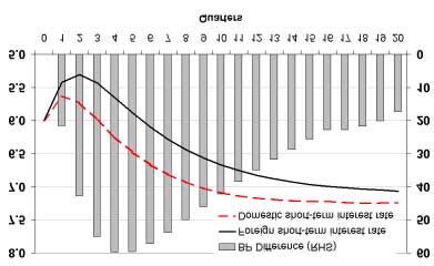
figure 5 which shows the resulting path for nominal short-term interest rates in the
sectors after a one-percentage point permanent increase in the inflation target.
3.3 Experiments undertaken
Four stochastic simulation experiments are conducted to explore the impact on the
New Zealand economy should it lose monetary policy independence. Under each
experiment two simulations are run. First, New Zealand operates under ‘status quo’
9
The difference in inflation target levels makes no difference to the simulation results, as
FPS is only concerned with the dynamic adjustment to deviations from equilibrium.10
independent (fully endogenous) monetary policy. Second, monetary policy is
exogenous to New Zealand being controlled by a foreign monetary authority. That is,
the foreign sector yield curve (solved for in the endogenous foreign sector of FPS) is
imported into the New Zealand model economy.
In the analysis, when interest rates are foreign controlled there is no UIP effect to
cause the nominal exchange rate to move between the domestic and foreign
economies. However, the real exchange rate will still adjust given shocks applied to it
in the stochastic simulation experiments. In general, the shocks applied result in the
real exchange rate moving in a counter-cyclical fashion, or in other terms, the real
exchange rate acts as a macroeconomic ‘stabiliser’.10
Each experiment consists of a 25 year simulation period with 100 draws of ‘typical’
macroeconomic shocks that New Zealand has experienced recently. This provides
10,000 observations for calculating measures of the average deviation from trend.
We explain the four shock experiments in turn. In the first experiment the New
Zealand economy is hit with domestic specific shocks to consumption, the real
exchange rate, inflation, and investment. The shocks from ‘the rest of the world’
which impact on both the New Zealand economy and the foreign sector are shocks to
world export prices and world demand. We have labelled this experiment as ‘all
shocks’.
10
The shocks applied in the analysis include disturbances to domestic demand
(consumption and investment), world demand, terms of trade, domestic price inflation,
and the real exchange rate. The auto and cross-correlation structure of the shocks are
determined by a VAR system estimated over the 1990s. In the VAR system the real
exchange rate acts in a stabilising fashion. For example, as is seen in Drew and Hunt
(1998), it appreciates following a positive impulse to domestic demand, world demand,
and the terms of trade. Similarly, the VECM-based work of Conway and Franulovich
(2002) concludes that the NZD/AUD real exchange rate acts as an effective shock
absorber rather than as a source of shock. These results are in contrast to econometric
evidence of ‘orbitals’ presented in Bowden and Grimes (2000), who conclude that the
real exchange rate does not buffer movements in the terms of trade. The VAR and
VECM evidence also runs against Coleman’s (1999) evaluation of the modern literature
on currency union, which suggests that in a low inflation environment exchange rate
volatility may be a cause rather than a means of adjusting to economic shocks.11
The second experiment subjects the New Zealand economy to shocks solely of
domestic origin i.e. terms of trade and world demand shocks are excluded. This gives
a better indication of what the costs of a fixed currency arrangement might be when
the foreign monetary authority ‘looks through’ New Zealand specific macroeconomic
disturbances. We have labelled this experiment as ‘domestic shocks’.
The third experiment subjects the New Zealand economy and the foreign sector to
shocks emanating solely from ‘the rest of the world’. That is, these shocks do not
originate in the potential currency union. The types of shocks we are considering in
this experiment are terms of trade and world demand shocks. The experiment with
‘rest of the world shocks’ is the opposite of the second experiment above.
The fourth experiment assumes that the New Zealand economy and the foreign sector
experience world shocks all of the time, but three out of ten years the New Zealand
business cycle goes out of phase as it is hit with domestic specific shocks. This
experiment attempts to incorporate empirical evidence surrounding the degree of
synchronisation of New Zealand’s business cycle with the rest of the world. For
example, Hall, Kim and Buckle (1998) find that New Zealand’s business cycle is
around 70 percent correlated with that of the USA over the late 1970s to the mid
1990s. Furthermore, concordance analysis by McCaw and McDermott (2000) over
the period 1960-99 revealed that the proportion of time that New Zealand’s business
cycle was in the same phase with those of Australia and the United States was about
70 percent. We have called this scenario ‘mixed shocks’.
3.4 Results
Table 2 provides the absolute and relative deterioration in the central bank’s ‘societal
loss’ under the four shock scenarios, while table 3 (and figure 6) presents the average
volatility outcomes. In table 2 the losses are calculated using a standard quadratic loss
function of the form:
( ) ( )
∞
L = ∑ (1 − λ ) y t − y * t
2 2
+λ π t − π T
t =1
( )
where y − y * is the output gap, π is annual CPI inflation, π T is the Reserve Bank
target rate of inflation (1.5 percent), and λ is the relative weight on inflation versus12
output variability. This is set at 1/2, which presumes the central bank cares as much
about inflation being away from the target as output being away from the economy’s
supply potential.11 Placing a higher weight on inflation deviating from the target
would represent a ‘hawkish’ central bank’s preferences; in contrast, a ‘dovish’ central
bank would place a higher weight on output deviating from potential.
The societal loss function described above is used as an illustrative metric and is not
part of any formal optimisation problem. Moreover, the choice of λ is somewhat
arbitrary and not derived explicitly from any optimisation problem.
The volatility in both output and inflation is the lowest, and therefore the loss is also
the lowest, under the scenario where the New Zealand economy experiences only
domestic shocks and operates a separate monetary policy. At the opposite end of the
spectrum, the loss is the highest when all shocks occur and monetary policy is foreign
controlled.
The societal loss under domestic policy is significantly different (at the 1 percent
significance level) to the societal loss under foreign policy. The F statistics for the
null hypothesis of no difference in loss when there are domestic, world, mixed and all
shocks imposed on the model are 3.73, 2.20, 2.05, and 1.71, respectively. All of these
test results are greater than the 1 percent critical value of 1.59.
The results are also not overly sensitive to the choice of λ . For any value of λ
between 0 and 1, the societal losses under domestic and foreign policy are
significantly different (at the 1 percent significance level) when the model is subjected
to domestic, world and mixed shocks. When the model is subjected to all shocks, the
difference is statistically significant at the 5 percent level for all values of λ (and at
the 1 percent level for 0 < λ < 0.6).
Intuitively, the loss under the domestic shocks and separate monetary policy scenario
should be the lowest as there are the least amount of shocks to contend with, and
11
Econometric evidence presented in Drew and Plantier (2000) is not inconsistent with the
Reserve Bank of New Zealand placing an equal weight on output and inflation deviations13
policy is geared towards responding to them. In stark contrast, in the case where only
domestically generated shocks occur, and the foreign central bank sets policy, the
variability in inflation is the highest seen (table 3). In losing monetary policy setting
ability, inflation variability increases four-fold, from 0.5 to 2 percent, while output
variability increases from 1.3 to around 2 percent. The overall deterioration in
performance is such that the loss arising from inflation and output variability
increases around 300 percent (table 2). The reason why inflation is notably more
volatile under this scenario is because it is the only one where monetary policy is
playing no buffering role. Under all other simulations, whether it is the foreign or
domestic central bank setting interest rates, there is some leaning against inflation
pressures.
Out of all the cases where monetary policy is set in the foreign sector, the volatility in
output and inflation is the lowest when the model is hit with solely world shocks. Not
surprisingly, this implies that under common shocks from the rest of the world,
foreign monetary policy is more appropriate. However, the deterioration in loss
associated with losing policy independence in this case is still significant at over 100
percent.
A final inference that can be drawn from the stochastic analysis is that, given the
shocks applied and the model, the cost of losing monetary policy independence is felt
more in terms of a deterioration in inflation performance than output performance.
The increase in output variability lies in a band of around 0.4 to 0.6 percent, whereas
the increase in inflation variability lies between 0.8 to 1.5 percent. These results
suggest that, overall, the more a central bank and society care about inflation control,
the less advisable it would be to enter into a common currency arrangement.
Conversely, if the costs of inflation variability are low, and there are large efficiency
gains to be had from entering into a common currency arrangement, then that could
well outweigh any increase in the variability of output associated with a loss of
monetary policy independence.
when setting monetary policy.14
4 Summary and conclusions
Deterministic simulations show that New Zealand’s output gap measure would have
been on average 0.3 percentage points higher than New Zealand’s actual historical
experience, if the more stimulatory Australian monetary conditions had been applied
to New Zealand during the 1990s. By 2000, though, output would have been
approximately back to baseline. This greater excess demand pressure would have led
to, on average, 1 percent higher CPI inflation. This implies that the Reserve Bank’s
previous 0 to 2 percent inflation target band would have been exceeded by a greater
amount, and for a greater number of periods than was actually the case. Moreover,
the current 0 to 3 percent band would have been exceeded over the last two quarters
of 1996. These outcomes eventuate despite the advantage of a conservative exchange
rate pass-through assumption.
Stochastic simulation results show that the volatility in output and inflation are the
lowest under the case where the New Zealand economy experiences domestic shocks
and operates its own monetary policy. In contrast, volatility is the highest when
domestic and world shocks occur, and New Zealand’s monetary policy is controlled
offshore. Moreover, irrespective of the shock scenario considered, model results
show the volatility in output and inflation to be greater under a common currency
policy environment than with New Zealand operating its own monetary policy.
In utilising these counterfactual model-based outcomes to assist judgement on
whether New Zealand should consider adopting some form of common currency, our
research suggests it is necessary to consider:
• outcomes from a representatively wide range of possible stochastic shocks, as well
as from the shocks which have occurred during one specified historical period,
and
• results not just for output and inflation, but also for their relative variability.
It follows, therefore, that any summary conclusion from the above system-wide
macroeconomic evidence will depend on the relative weighting placed on the degree
of variability of inflation and output. If a high weight is placed on avoiding such15 variability, then our results imply a common currency should not be adopted, and New Zealand should retain its ability to set monetary policy independent of that set in Australia.
16

Appendix: Modelling framework
The potential effects of New Zealand adopting a foreign currency are analysed using
the core model of the Reserve Bank of New Zealand’s Forecast and Policy System
(FPS).12 This appendix provides an overview of the model used to generate
counterfactual paths for output and inflation, under the assumption that New Zealand
had Australian monetary conditions through the 1990s. The implications of whether
New Zealand had joined a currency union with Australia, or simply adopted the
Australian dollar (i.e. dollarised) can be analysed the same way. Because Australia
has six times the population of New Zealand and higher per-capita GDP the New
Zealand business cycle conditions would be of secondary importance in setting
monetary conditions.        Australian monetary conditions would therefore have
dominated in either case.

FPS describes the interaction of five economic agents: households, firms, government,
a foreign sector, and the monetary authority. The model has a two-tiered structure.
The first tier is an underlying steady-state structure that determines the long-run
equilibrium to which the model will converge.            The second tier is the dynamic
adjustment structure that traces out how the economy converges towards that long-run
equilibrium.

The long-run equilibrium is characterised by a neo-classical balanced growth path.
Along that growth path, consumers maximise utility, firms maximise profits and
government achieves exogenously-specified targets for debt and expenditures. The
foreign sector trades in goods and assets with the domestic economy. Taken together,
the actions of these agents determine expenditure flows that support a set of stock
equilibrium conditions that underlie the balanced growth path.

The dynamic adjustment process overlaid on the equilibrium structure embodies both
‘expectational’ and ‘intrinsic’ dynamics. Expectational dynamics arise through the
interaction of exogenous disturbances, policy actions and private agents’ expectations.
Policy actions are introduced to re-anchor expectations when exogenous disturbances

12
     See Black et al (1997), and Hunt et al (2000), for a more complete description of the FPS
     model.
17 move the economy away from equilibrium. Because policy actions do not immediately re-anchor private expectations, real variables in the economy must follow dis-equilibrium paths until expectations return to equilibrium. To capture this notion, expectations are modelled as a linear combination of a backward-looking autoregressive process and a forward-looking model-consistent process. Intrinsic dynamics arise because adjustment is costly, and these costs are modelled using a polynomial adjustment framework. In addition to expectational and intrinsic dynamics, the behaviour of both the monetary and fiscal authorities also contributes to the overall dynamic adjustment process. In FPS, goods are differentiated by a system of relative prices. Overlaid on this system of relative prices is an inflation process. While inflation can potentially arise from many sources in the model, it is fundamentally the difference between the economy’s supply capacity and the demand for goods and services that determines inflation in domestic prices. Further, the relationship between goods market dis- equilibrium and inflation is specified to be asymmetric. Excess demand generates more inflation than the deflation caused by an identical amount of excess supply. A.1 Households There are two types of households in the model: ‘rule-of-thumb’ and ‘forward- looking’. Forward-looking households hold all of the economy’s financial assets and, on average, save. Rule-of-thumb households spend all their disposable income each period and hold no assets. The theoretical core of the household sector is the specification of the optimisation problem for forward-looking households. The specification is based on the overlapping generations framework of Yaari (1965), Blanchard (1985), Weil (1989) and Buiter (1988), but in a discrete time form as in Frenkel and Razin (1992) and Black et al (1994). In this framework, the forward- looking household chooses a path for consumption – and a path for savings – that maximises the expected present value of lifetime utility subject to a budget constraint and a fixed birth-rate. This basic equilibrium structure is overlaid with polynomial adjustment costs, the influence of monetary policy, an asset dis-equilibrium term, and an income-cycle effect.
18

The population size and age structure is determined by the simplest possible
demographic assumptions. We assume that new consumers enter according to a fixed
birth rate and that existing consumers exit the economy according to the fixed
probability of death. For the supply of labour, we assume that each consumer offers a
unit of labour services each period. That is, labour is supplied inelastically with
respect to the real wage.

A.2        The representative firm
The formal introduction of a supply side requires us to go beyond the simple
endowment economy of the Blanchard et al framework. The firm is modelled very
simply in FPS, but as with the characterisation of the consumer, some extensions are
made to capture essential features of the economy. Investment and capital formation
are modelled from the perspective of a representative firm.         This firm acts to
maximise profits subject to the usual accumulation constraints. Firms are assumed to
be perfectly competitive, with free entry and exit to markets. Firms produce output,
pay wages for labour input, and make rental payments for capital input.13          The
production technology is Cobb-Douglas, with constant returns to scale. Profit
maximisation is sufficient to determine the level of output, the level of employment,
and the real wage. FPS extends this framework in a number of directions as firms
face adjustment costs for capital and a time-to-build constraint.

A.3        The Government
Government has the power to collect taxes, raise debt, make transfer payments, and
purchase output. As with households and firms, the structure of the model requires
clear objectives for government in the long run. However, whereas households’ and
firms’ objectives arise through explicit maximisation, we directly impose fiscal policy
choices for debt and expenditure. The government’s binding intertemporal budget
constraint is used to solve for the labour income tax rate that supports the fiscal
choices.     The interactions of debt, spending and taxes create powerful effects
throughout the rest of the model; government is non-neutral.

13
      We also assume that households own the capital stock.
19
A.4 The Monetary Authority
The monetary authority effectively closes the model by enforcing a nominal anchor.
Its behaviour is modelled by a forward-looking reaction function that moves the short-
term nominal interest rate in response to projected deviations of inflation from an
exogenously specified target rate. The reaction function can be expressed as:
( )
8
rnt − rnlt = rnt* − rnlt* + ∑1.4 π te+ i − π T
i =6
where rn and rnl are short and long nominal interest rates, respectively; rn * and
rnl * are their equilibrium equivalents; π te+i is the model consistent projection of
inflation i quarters ahead, and π T is the policy target.14 Although the reaction
function is ad hoc in the sense that it is not the solution to a well-defined optimal
control problem as in Svensson (1997), its design is not totally arbitrary. The
forward-looking nature (i.e. 6-8 quarters ahead) of the reaction function respects the
lags in the economy between policy actions and their subsequent implications for
inflation outcomes. Further, the strength of the policy response to projected deviations
in inflation (1.4) implicitly embodies the notion that the monetary authority is not
single minded in its pursuit of the inflation target. Other factors such as the variability
of its instrument and the variability of the real economy are also of concern.
A.5 The foreign sector
The foreign sector is a stylised representation of a foreign economy, not necessarily
the United States or Australia. The foreign sector is treated as completely exogenous
to the domestic economy. It supplies the domestic economy with imported goods and
purchases the domestic economy’s exports, and thus completes the demand side of the
model. Further, the foreign sector stands ready to purchase assets from, or sell assets
to, domestic households – depending on whether households choose to be net debtors
or net creditors relative to the rest of the world.
14
The terms of the current Policy Targets Agreement, signed between the Governor of the
Reserve Bank of New Zealand and the Treasurer, dictates that the Reserve Bank target an
inflation band of 0 to 3 percent. In FPS the policy target is the mid-point of this band,
i.e. 1.5 percent.20
A simplified summary of the key foreign sector model equations is presented below.
The equations denoted with an arrow illustrate a subtle re-calibration of the foreign
sector to match the properties of the domestic central bank reaction function.
IS curve:
(y − y ) ( ) ( )
2
= δ y − y* t −1 − ∑ γ i r − r
* *
t t −i
i =1
( ) ( ) ( )
2
⇒ y − y* t = δ y − y* t −1 − ∑ γ i rsl − rsl * t −i
i =1
Phillips curve:
π t = π te + ∑ α i (y − y * )t −i
2
i =0
Inflation expectations:
4 4
π te = ϖ 1 ∑η iπ t −i + (1 − ϖ 1 )∑η iπ t +i
i =1 i =1
Long-term inflation expectations:
π tle = 0.20(π te+ 4 + π te+8 + π te+12 + π te+16 + π te+ 20 )
Reaction function:
[( )( ) ] ( )
8
rnt = 1 + rt* 1 + π T − 1 + ∑ 2.5 π te+ i − π T
i =6
( )
8
⇒ rnt − rnlt = rnt* − rnlt* + ∑1.4 π te+ i − π T
i =6
Fisher equation:
1 + rnt
rt = − 1
1+πt
e
21
Long nominal interest rate:
1 + tp t* 1 + rnt
0.05
rnl t = ε (1 + rnl t +1 )
+ *
+
− 1 [( )( ) ]
+ (1 − ε ) 1 + rlt* 1 + π T − 1
1 tp t +1 1 rn t + 20
Fisher equation:
1 + rnl t
rl t = − 1
1+πt
le
where:
(y − y )
*
t is the output gap at time t;
π t is annual inflation at time t;
π te is expected inflation at time t;
π tle is long-term expected inflation at time t;
π T is the policy target;
rnt is the nominal interest rate at time t;
rt is the interest rate at time t;
rnl t is the nominal long-term interest rate at time t;
rl t is the long-term interest rate at time t;
rt* is the equilibrium interest rate at time t;
rl t* is the equilibrium long-term interest rate at time t;
rnt* is the equilibrium nominal interest rate at time t;
rnlt* is the equilibrium nominal long-term interest rate at time t;
rsl t* is the equilibrium yield gap at time t;
rsl t is the yield gap at time t;
(r − r ) is the interest rate gap i.e actual less equilibrium at time t;
*
t
(rsl − rsl ) is the yield curve gap i.e actual less equilibrium at time t;
*
t
tp t* is the equilibrium term premium at time t.22
References
Bjorksten, N (2001), ‘The current state of New Zealand monetary union research’,
Reserve Bank of New Zealand Bulletin, 64 (4), 44-55.
Black, R, D Laxton, D Rose and R Tetlow (1994), ‘The Steady-State Model:
SSQPM.’ The Bank of Canada’s New Quarterly Projection Model, Part 1,
Technical Report, (72), Ottawa: Bank of Canada.
Black, R, V Cassino, A Drew, E Hansen, B Hunt, D Rose and A Scott (1997), ‘The
Forecasting and Policy System: the core model’, Reserve Bank of New
Zealand Research Paper (43).
Blanchard, O J (1985), ‘Debt, deficits and finite lives’, Journal of Political Economy
93, 223–247.
Bowden, R (2000), ‘Tasman or Pacific? The case for a multilateral USD connection’,
Victoria Economic Commentaries, October, 8-16.
Bowden, R and A Grimes (2000), ‘Welfare effects of currency integration’, presented
to the Annual Conference of the New Zealand Association of Economists,
Wellington, July.
Buiter, W H (1988), ‘Death, birth, productivity growth and debt neutrality’, The
Economic Journal, 98, (391), 279-293.
Coleman, A (1999), ‘Economic Integration and Monetary Union’, New Zealand
Treasury Working Paper 99/6, Wellington.
Coleman, A (2001), ‘Three Perspectives on an Australasian Monetary Union’ Future
Directions for Monetary Policies in East Asia, D. Gruen and J. Simon, eds.,
Reserve Bank of Australia, Sydney, 156-188.
Conway, P and R Franulovich (2002), ‘Explaining the NZ-Australian exchange rate’,
Westpac Institutional Bank Occasional Paper, April, www.wib.westpac.co.nz.
Crosby, Mark and Glenn Otto (2000), ‘An Australia New Zealand Currency Union?’
prepared for Financial Markets and Policies in East Asia Conference,
Australian National University, Canberra, September.
Drew, A, and B Hunt (1998), ‘The Forecasting and Policy System: stochastic
simulations of the core model’, Reserve Bank of New Zealand Discussion
Paper G98/6.
Drew, A, and B Hunt (2000), ‘Efficient Simple Policy Rules and the Implications of
Potential Output Uncertainty’, Journal of Economics and Business, 52, 143-
160.23
Drew, A and C Plantier (2000), ‘Interest rate smoothing in New Zealand and other
dollar block countries’, Reserve Bank of New Zealand Discussion Paper
DP2000/10.
Frenkel, J and A Razin (1992), Fiscal Policies and the World Economy, Cambridge:
MIT Press.
Grimes, A (2000), ‘Case for a world currency: Is an ANZAC Dollar a Logical Step?’
Victoria Economic Commentaries, October, 17-26.
Grimes, A, F Holmes and R Bowden (2000), An ANZAC Dollar? Currency Union and
Business Development, Institute of Policy Studies, Wellington.
Hall, V B, K Kim and R A Buckle (1998), ‘Pacific Rim Business Cycle Analysis:
Synchronisation and Volatility’, New Zealand Economic Papers, 32 (2), 129-
160.
Hargreaves, D and C J McDermott (1999), ‘Issues relating to optimal currency areas:
theory and implications for New Zealand’, Reserve Bank of New Zealand
Bulletin, 62 (3), 16-29.
Hartley, P (2001), ‘Monetary arrangements in New Zealand’, New Zealand Business
Roundtable, Wellington, May.
HSBC: Economics (1999), ‘Convergence: The Australasian economy in the new
decade’, HSBC Securities (Australia) Limited, December.
Hunt, B, D Rose and A Scott (2000), ‘The core model of the Reserve Bank of New
Zealand's Forecasting and Policy System’, Economic Modelling, 17, (2), 247-
274.
McCaw, S and C. J McDermott (2000), ‘How New Zealand adjusts to macroeconomic
shocks: implications for joining a currency area’, Reserve Bank of New
Zealand Bulletin, 63 (1), 35-51.
Mundell, R (1961), ‘A theory of optimum currency areas’, American Economic
Review, 51, 657-665.
Rose, A K and E van Wincoop (2001), ‘National money as a barrier to international
trade: The real case for currency union’, American Economic Review, 91, 386-
390.
Scrimgeour, D (2001), ‘Exchange rate volatility and currency union: Some theory and
New Zealand evidence’, Reserve Bank of New Zealand discussion paper,
DP2001/04.
Svensson, L E O (1997), ‘Inflation forecast targeting: Implementing and monitoring
inflation targets’, European Economic Review, 41, (6), 1111-1146.24
Weil, P (1989) ‘Overlapping families of infinitely-lived agents’, Journal of Public
Economics, 38, 183-198.
Yaari, M E (1965), ‘Uncertain lifetimes, life insurance, and the theory of the
consumer’, The Review of Economic Studies 32, 137-50.25
Table 1
Long-run properties of the foreign sector and the
domestic NZ sector in FPS
Long-run value
(percentage points)
Real short-term foreign interest rate 3.5
Real short-term domestic interest rate 4.5
Short-term foreign interest rate 6.0
Short-term domestic interest rate 6.0
Long-term foreign interest rate 6.5
Long-term domestic interest rate 6.5
Foreign yield gap -0.5
Domestic yield gap -0.5
Foreign inflation target 2.5
Domestic inflation target 1.5
Table 2
Collation of stochastic simulation volatility properties
into a standard loss function
(output and inflation variability are weighted equally)
Simulation Loss under Loss under Foreign Percentage
Domestic Policy Policy change in Loss
Domestic Shocks 1.0 3.8 273
World Shocks 1.3 2.9 120
Mixed Shocks 1.6 3.3 105
All Shocks 2.3 3.9 7126
Table 3
Average volatility properties for output gap and
inflation
(25 year simulation period – 100 shock draws – 10,000 observations)
(percentage point units)
Simulation: 80% Confidence 80% Confidence RMSD RMSD
Interval for Interval for CPI Output* CPI
Output Gap Inflation Inflation
Domestic shocks -1.7 to 1.7 0.8 to 2.2 1.340 0.517
& domestic policy
World shocks & -2.0 to 2.0 0.8 to 2.2 1.543 0.527
domestic policy
Mixed shocks & -2.2 to 2.2 0.7 to 2.3 1.689 0.595
domestic policy**
All shocks & -2.6 to 2.6 0.6 to 2.4 2.013 0.734
domestic policy
Domestic shocks -2.6 to 2.6 -0.9 to 3.9 2.010 1.909
& foreign policy
World shocks & -2.6 to 2.6 -0.2 to 3.2 2.011 1.346
foreign policy
Mixed shocks & -2.7 to 2.7 -0.3 to 3.3 2.143 1.409
foreign policy
All shocks & -3.0 to 3.0 -0.4 to 3.4 2.366 1.505
foreign policy
*
Root Mean Square Deviation. This is the average squared deviation in the
observed series from its control long-run equilibrium. The RMSD for output is
the averaged squared deviation in output from potential, and the long-run
equilibrium is zero ie the output gap is closed. The RMSD for inflation is the
average squared deviation in the Bank’s target measure of inflation from the mid-
point of the target range i.e. 1.5 percent.
**
Under the ‘mixed shocks’ simulations the average correlation (across the
draws) between the domestic and the foreign sector output gap is 0.72. This
suggests that our specification of mixed shocks captures the spirit of Hall et al
(1998), and McCaw and McDermott (2000) ie the finding that the New
Zealand business cycle is synchronised with that of the USA and Australia
around 70 percent of the time.27 Figure 1 New Zealand’s yield spread and Australian counterfactual scenario (percentage/basis points) Figure 2 New Zealand’s real exchange rate and Australian counterfactual scenario
28

Figure 3
Baseline output gap and Australian counterfactual
scenario
(percentage points)

Figure 4
The Reserve Bank’s target measure of annual
inflation and Australian scenario
(percentage points)

Note: The horizontal lines denote the Reserve Bank’s target band.
29

Figure 5
Interest rate response within the domestic and foreign
sectors after a 1 percent rise in their respective
inflation targets
(percentage points)

Figure 6:
Long-run average inflation and output volatility
(percentage point units)
You can also read