Federal Reserve Bank of Minneapolis
←
→
Page content transcription
If your browser does not render page correctly, please read the page content below
Federal Reserve Bank
      of Minneapolis

\ s
      P*: Not the Inflation
      Forecaster's Holy Grail (p. 3)
      Lawrence J. Christiano

      The U.S. Economy
      in 1990 and 1991:
      Continued Expansion
      Likely (p. 19)
      David E. Runkle

      A Simple Way to Estimate
      Current-Quarter GNP (p. 27)
      Terry J. Fitzgerald
      Preston J. Miller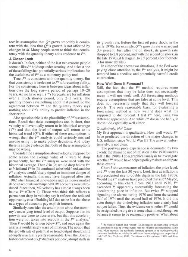
Federal Reserve Bank of Minneapolis

Quarterly Review
V o l . 1 3 , NO. 4   ISSN 0 2 7 1 - 5 2 8 7

This publication primarily presents economic research aimed at improving
policymaking by the Federal Reserve System and other governmental
authorities.

Produced in the Research Department. Edited by Preston J. Miller, Kathleen
S. Rolfe, and Inga Velde. Graphic design by Barbara Birr and Phil Swenson,
Public Affairs Department.

Address questions to the Research Department, Federal Reserve Bank,
Minneapolis, Minnesota 55480 (telephone 612-340-2341).

Articles may be reprinted if the source is credited and the Research
Department is provided with copies of reprints.

 The views expressed herein are those of the authors and not
necessarily those of the Federal Reserve Bank of Minneapolis or
the Federal Reserve System.
Federal Reserve Bank of Minneapolis
   Quarterly Review Fall 1989

   P*: Not the Inflation Forecaster's Holy Grail

   Lawrence J. Christiano
   Research Officer
   Research Department
   Federal Reserve Bank of Minneapolis

Last summer, the Board of Governors of the Federal           an economy, the number of dollars spent or received
Reserve System unveiled a new, experimental way to           equals the number of dollars changing hands. Since
forecast trends in inflation, which it calls P-Star (P*).    early in the century (Fisher 1911), economists have
The announcement received an enormous amount of              expressed this fact as the equation of exchange:
publicity throughout—and even outside—the United
States. One journalist captured the excitement and           (1)       PXQ       =      MXV
optimism generated by the new forecasting method
particularly well: "Economists have long been search-        where
ing for the holy grail—an accurate thermometer with                     P = the current price level
which to forecast inflation. . . . Some think they have                     (here, I'll use the implicit price deflator of gross
found it."1                                                                  national product, or GNP)
   They haven't. At first glance, P* may look like an                   Q = the current level of output, adjusted for
especially good way to forecast inflation. But a closer                     inflation
                                                                            (here, real GNP)
look raises doubts about that. And those doubts are
confirmed by some simple tests of its forecasting                      M — the current money supply
                                                                           (here, the Fed's M2 definition of money)2
ability. Had P* been used to forecast inflation in the
1970s and 1980s, its track record would not have been                   V = the velocity of money
much better than those of other forecasting methods.                        (the number of times each dollar of the money
                                                                             supply is spent each year).
While P* may not be a bad way to forecast inflation, it is
certainly not an exceptionally good way either.
                                                                 t Revision of a speech to the Board of Directors of the Federal Reserve Bank
What's So Appealing About P * ?                              of Minneapolis on November 16,1989. The speech updates the author's report
This new inflation forecasting method is appealing to        of December 12, 1988. The author has benefited from comments by Jeffrey
                                                             Hallman, Richard Porter, and David Small.
many people because it is fairly simple, it seems to             J
                                                                   The Board's new forecasting method is described in Hallman, Porter, and
make sense, and it is consistent with a widely respected     Small 1989. The above quotation is from the Economist (Business/Economics
theory of what causes inflation in the long run.             focus, 1989). Other P* publicity includes a front-page story in the New York
                                                             Times (Kilborn 1989), two stories in the business section of a Sunday New York
It's    Simple...                                            Times (Hunt 1989 and Lee 1989), and stories in Business Week (McNamee
                                                             1989) and the American Banker (Heinemann 1989).
As an inflation forecasting method, P* can be described          2
                                                                   M2 includes (1) the components of the Fed's Ml definition of money
with just a few simple equations.                            [currency held by the public, travelers' checks of nonbank issuers, demand
     One equation states an obvious fact: at any time in     deposits at banks and thrifts, negotiable order of withdrawal (NOW and Super-

                                                                                                                                           3
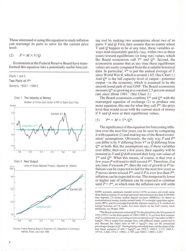
Those interested in using this equation to study inflation                       ing tool by making two assumptions about two of its
can rearrange its parts to solve for the current price                           parts: V and Q. First, they assume that no matter where
level:                                                                           V and Q happen to be at any time, these variables al-
                                                                                 ways tend reasonably quickly (say, within two or three
(2)         P = MX           V/Q.                                                years) toward equilibrium (or long-run) values, which
                                                                                 the Board economists call V* and Q*. Second, the
   Economists at the Federal Reserve Board have trans-                           economists assume that at any time these equilibrium
formed this equation into a potentially useful forecast-                         values are easily computed from the available historical
                                                                                 data. In particular, V* is just the annual average of V
Charts 1 and 2                                                                   since World War II, which is around 1.65. (See Chart 1.)
                                                                                 And Q* is the full capacity level of output—potential
Two Parts of P *                                                                 output—in the economy, which is assumed to be the
Quarterly, 1959:1-1989:3                                                         smooth trend path of real GNP. The Board economists
                                                                                 measure Q* as growing at a constant 2.5 percent annual
                                                                                 rate since about 1981.3 (See Chart 2.)
      Chart 1 The Velocity of Money                                                 The Board economists combine V* and 0 * with the
                 Number of Times Each Dollar of M2 Is Spent Each Year            rearranged equation of exchange (2) to produce one
                                                                                 more equation, this one for what they call P*: the price
                                                                                 level that would occur with the current stock of money
                                                                                 if V and Q were at their equilibrium values,

                                                                                 (3)        P* = MX              V*/Q*.

                                                                                     The significance of this equation for forecasting infla-
                                                                                 tion over the next few years can be seen by comparing
                                                                                 it with equation (2) and making use of the Board econo-
                                                                                 mists' assumptions. Obviously, the only way P and P*
                                                                                 can differ is by V differing from V* or Q differing from
                                                                                 (2* or both. But, the assumptions say, if these variables
                                                                                 ever differ, then over a few years, their equality will be
                                                                                 restored as V and Q drift toward their long-run values of
                                                                                 V* and Q*. What this means, of course, is that over a
      Chart 2 Real Output                                                        few years P will tend to drift toward P*. Therefore, if at
Trii. of         Level    Gross   National Product, Adjusted for Inflation       any time P exceeds P*, then the rate of growth in P (in-
                                                                                 flation) can be expected to fall for the next few years as
                                                                                 P moves down toward P*; and if Pis ever less than P*,
                                                                                 inflation can be expected to rise. This temporarily lower
                                                                                 or higher rate of inflation can be expected to continue
                                                                                 until P = P*, at which time the inflation rate will settle

                                                                                 NOW) accounts, automatic transfer service (ATS) accounts, and credit union
                                                                                 share draft accounts], (2) savings and small-denomination (less than $ 100,000)
                                                                                 time deposits, (3) money market deposit accounts (MMDAs), (4) shares in
                                                                                 noninstitutional money market mutual funds, (5) overnight repurchase agree-
                                                                                 ments (RPs), and (6) overnight Eurodollar deposits issued to U.S. residents by
                                                                                 foreign branches of U.S. banks. For more details on the Fed's money stock
                                                                                 definitions, see Walter 1989.
                                                                                     3
                                                                                       The Board economists estimated Q* for the period from the first quarter of
                                                                                  1952 (1952:1) to the third quarter of 1989 (1989:3). To see how their measure
                                                                                 of Q* is constructed, it is revealing to look not directly at Q*, but rather at 400 X
                                                                                 log(@*). This is simply four straight lines, with different slopes, joined end to
                                                                                 end. Because the slopes refer to 400 X log(£?*), they are the annualized
                                                                                 percentage changes in Q*. The beginning and ending dates and the slopes of the
     Sources: Federal Reserve Board of Governors; U.S. Department of Commerce;   four linear segments of 400 X log(0*) are 1952:1-1965:2, 3.373; 1965:3-
              Hallman, Porter, and Small 1989                                     1973:4,3.466; 1974:1-1980:1, 2.795; and 1980:2-1989:3,2.497.

4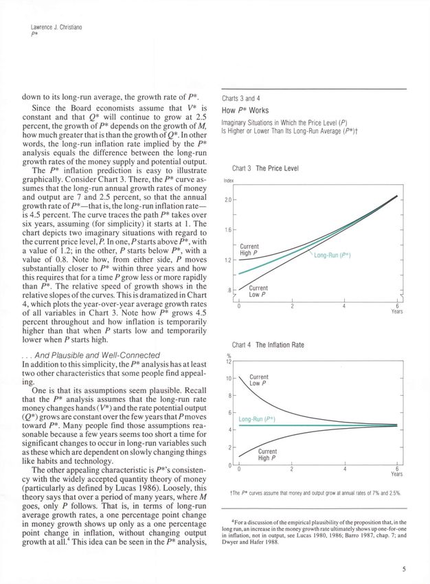
Lawrence J. Christiano
   P*

down to its long-run average, the growth rate of P*.           Charts 3 and 4
    Since the Board economists assume that V* is               How P * Works
constant and that
too: its assumption that Q* grows smoothly is consis-         its growth rate. Before the first oil price shock, in the
tent with the idea that Q*'s growth is not affected by        early 1970s, for example, Q*'s growth rate was around
changes in M. Many people seem to think that consis-          3.4 percent. Just after the oil shock, its growth rate
tency with the quantity theory adds credence to P*.           dropped to 2.8 percent, and with the second oil shock, in
A Closer Look                                                 the late 1970s, it fell again, to 2.5 percent. (See footnote
It doesn't. In fact, neither of the last two reasons people   3 for more details.)
seem to like P* holds up under scrutiny. And at least one         In either of the above two situations, if the Fed were
of these failings has potentially serious implications for    paying close attention to the P* analysis, it might be
the usefulness of P* as a monetary policy tool.               tempted into a needless and potentially harmful credit
    True, P* is consistent with the quantity theory. But      contraction.
that consistency is irrelevant to P*'s forecasting ability.   How Well Does It Forecast?
For the consistency here is between ideas about infla-        Still, the fact that the P* method requires some
tion over the long run—a period of perhaps 10-20              assumptions that may be false does not necessarily
years. As we have seen, P*'s forecasts are for inflation      mean it will not work well. All forecasting methods
over a much shorter period, only 2 - 3 years. The             require assumptions that are false at some level. This
quantity theory says nothing about that period. So the        does not necessarily imply that they will forecast
agreement between P* and the quantity theory says             poorly. The only reasonable basis for evaluating a
nothing about P*'s ability to predict inflation in the        forecasting method is how well it does what it's
shorter run.                                                  supposed to do: forecast. I test P* here, using two
    Also questionable is the plausibility of P*'s assump-     different approaches. And while P* doesn't do badly, it
tions. Recall that these assumptions are, in short, that      doesn't do especially well either.
velocity will eventually return to its historical average
(V*) and that the level of output will return to its          Qualitatively, Not Clear
historical trend (2*). If either of these assumptions is      My first approach is qualitative. How well would P*
wrong, then the P* analysis could seriously mislead           have predicted the direction of the major changes in
anyone using it to make policy decisions. And today           U.S. inflation since World War II? The answer, unfor-
there is ample evidence that both of these assumptions        tunately, is not clear.
may be wrong.                                                    The postwar price experience is dominated by two
    Consider the assumption about velocity. Suppose for       events: the dramatic rise of inflation in the 1970s and its
some reason the average value of V were to drop               fall in the 1980s. I do a graphical analysis to investigate
permanently, but the P* analysis were used with the           whether P* would have helped policymakers anticipate
historical average. Then P in (2) would drop below P*         these events.
as Vfell and V* in (3) continued to be held fixed, and the       Chart 5 shows measures of inflation, the price level,
P* analysis would falsely signal an imminent danger of        and P* over the last 30 years. Look first at inflation's
inflation. Actually, this may have happened after late        unprecedented rise to double digits in the late 1970s.
1982 when financial innovations such as money market          Would the P* analysis have predicted that rise? Maybe,
deposit accounts and Super-NOW accounts were intro-           according to this chart. From 1963 until 1970, P*
duced. Since then, M2 velocity has almost always been         exceeded P} apparently successfully forecasting the
below V* (Chart 1). Those who think this reflects a           accelerating pace in inflation. But twice P* stopped
permanent drop in velocity say it reflects the reduced        signaling the alarm: during 1970 and from the second
opportunity cost of holding M2 due to the fact that these     half of 1974 until the second half of 1976. It did this
new types of accounts pay explicit interest.                  even though the underlying inflation rate clearly had
    Similarly, consider the assumption about the econo-       not yet fallen. Thus, the evidence on whether P* would
my's underlying trend level of output. Suppose that its       have signaled the big rise is somewhat mixed, though on
growth rate were to accelerate, but that this accelera-       balance it seems to be reasonably positive. What about
tion were not taken into account in the P* analysis.5
Then P would be driven below P*, and once again the                5
                                                                     The work of Nelson and Plosser (1982) suggests another sense in which
analysis would falsely warn of inflation. The notion that     this assumption may be wrong: output may not revert to any underlying, stable
                                                              trend. More recently, the academic literature appears to be moving toward a
the growth rate of potential or trend output should shift     consensus that little can reliably be said about the underlying trend properties of
abruptly is actually pretty reasonable. Even the Board's      real GNP. See Cochrane 1988, Christiano and Eichenbaum 1989, and Sims
historical record of Q* displays periodic, abrupt shifts in   1989.

6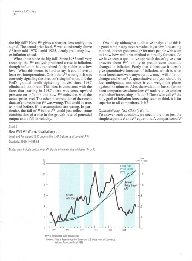
Lawrence J. Christiano
    p*

the big fall? Here P* gives a sharper, less ambiguous                                        Obviously, although a qualitative analysis like this is
signal. The actual price level, P, was consistently above                                 a good, simple way to start evaluating a new forecasting
P* from mid-1978 to mid-1985, clearly predicting low-                                     method, it is not good enough for most people who want
er inflation ahead.                                                                       to know how well that method can really forecast. As
   What about since the big fall? Since 1985 until very                                   we have seen, a qualitative approach doesn't give clear
recently, the P* analysis predicted a rise in inflation,                                  answers about P*'s ability to predict even dramatic
though inflation has remained fairly stable at a low                                      changes in inflation. Partly that is because it doesn't
level. What this means is hard to say. It could have at                                   give quantitative forecasts of inflation, which is what
least two interpretations. One is that P* was right. It was                               most forecasters want anyway: how much will inflation
correctly signaling the threat of rising inflation, and the                               change and when? A quantitative analysis should be
Fed's gradual credit-tightening moves since 1987                                          less ambiguous, too, since it can weigh the pluses
eliminated the threat. This idea is consistent with the                                   against the minuses. Also, the evaluation has so far not
facts that starting in 1987 there was some upward                                         been comparative; where does P* rank relative to other
pressure on inflation and now P* coincides with the                                       methods of forecasting inflation? Those who call P* the
actual price level. The other interpretation of the recent                                holy grail of inflation forecasting seem to think it is far
data, of course, is that P* was wrong. This could be true,                                superior to all competitors. Is it?
as noted before, if its assumptions are wrong. In par-
ticular, the fall of P below P* could just reflect some                                   Quantitatively, Not Clearly Better
combination of a rise in the growth rate of potential                                     To answer such questions, we need more than just the
output and a fall in velocity.                                                            simple separate P and P* equations. A comparison of P

Chart 5
How Well P * Works: Qualitatively . . .
Level and Annualized % Change in the GNP Deflator and Level of P*t
Quarterly, 1959:1-1989:3

Shaded areas indicate periods when P* signals an imminent rise in inflation (P*>P).

                                  f P * is constructed using equation (3).
                                   Sources: Federal Reserve Board ot Governors; U.S. Department of Commerce;
                                            Hallman, Porter, and Small 1989

                                                                                                                                                    7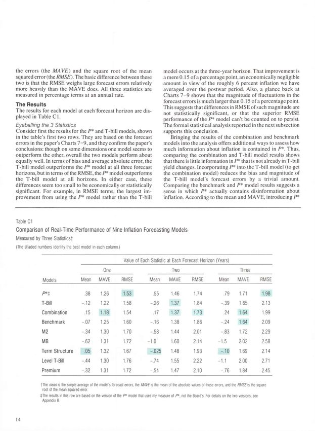
and P* can suggest the direction in which inflation will through the third quarter of 1989. To evaluate the
be moving, but not how much it will move or when. To models' longer-run performance, I also computed sets
determine things like that, we must build P and P* into of two- and three-year-ahead forecasts in the same
an explicit statement of what determines future infla- way. (For technical details of my procedures, see
tion and how, that is, into a mathematical model. Appendix B.)7
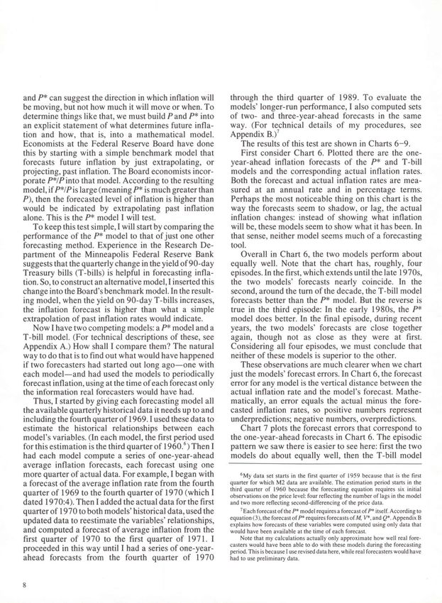
Economists at the Federal Reserve Board have done The results of this test are shown in Charts 6-9.
this by starting with a simple benchmark model that First consider Chart 6. Plotted there are the one-
forecasts future inflation by just extrapolating, or year-ahead inflation forecasts of the P* and T-bill
projecting, past inflation. The Board economists incor- models and the corresponding actual inflation rates.
porate P*/Pinto that model. According to the resulting Both the forecast and actual inflation rates are mea-
model, if P*/Pis large (meaning P* is much greater than sured at an annual rate and in percentage terms.
P), then the forecasted level of inflation is higher than Perhaps the most noticeable thing on this chart is the
would be indicated by extrapolating past inflation way the forecasts seem to shadow, or lag, the actual
alone. This is the P* model I will test. inflation changes: instead of showing what inflation
To keep this test simple, I will start by comparing the will be, these models seem to show what it has been. In
performance of the P* model to that of just one other that sense, neither model seems much of a forecasting
forecasting method. Experience in the Research De- tool.
partment of the Minneapolis Federal Reserve Bank Overall in Chart 6, the two models perform about
suggests that the quarterly change in the yield of 90-day equally well. Note that the chart has, roughly, four
Treasury bills (T-bills) is helpful in forecasting infla- episodes. In the first, which extends until the late 1970s,
tion. So, to construct an alternative model, I inserted this the two models' forecasts nearly coincide. In the
change into the Board's benchmark model. In the result- second, around the turn of the decade, the T-bill model
ing model, when the yield on 90-day T-bills increases, forecasts better than the P* model. But the reverse is
the inflation forecast is higher than what a simple true in the third episode: In the early 1980s, the P*
extrapolation of past inflation rates would indicate. model does better. In the final episode, during recent
Now I have two competing models: a P* model and a years, the two models' forecasts are close together
T-bill model. (For technical descriptions of these, see again, though not as close as they were at first.
Appendix A.) How shall I compare them? The natural Considering all four episodes, we must conclude that
way to do that is to find out what would have happened neither of these models is superior to the other.
if two forecasters had started out long ago—one with These observations are much clearer when we chart
each model—and had used the models to periodically just the models' forecast errors. In Chart 6, the forecast
forecast inflation, using at the time of each forecast only error for any model is the vertical distance between the
the information real forecasters would have had. actual inflation rate and the model's forecast. Mathe-
Thus, I started by giving each forecasting model all matically, an error equals the actual minus the fore-
the available quarterly historical data it needs up to and casted inflation rates, so positive numbers represent
including the fourth quarter of 1969.1 used these data to underpredictions; negative numbers, overpredictions.
estimate the historical relationships between each Chart 7 plots the forecast errors that correspond to
model's variables. (In each model, the first period used the one-year-ahead forecasts in Chart 6. The episodic
for this estimation is the third quarter of 1960.6) Then I pattern we saw there is easier to see here: first the two
had each model compute a series of one-year-ahead models do about equally well, then the T-bill model
average inflation forecasts, each forecast using one
more quarter of actual data. For example, I began with 6
My data set starts in the first quarter of 1959 because that is the first
a forecast of the average inflation rate from the fourth quarter for which M2 data are available. The estimation period starts in the
third quarter of 1960 because the forecasting equation requires six initial
quarter of 1969 to the fourth quarter of 1970 (which I observations on the price level: four reflecting the number of lags in the model
dated 1970:4). Then I added the actual data for the first and two more reflecting second-differencing of the price data.
quarter of 1970 to both models' historical data, used the 7
Each forecast of the P* model requires a forecast of P* itself. According to
equation (3), the forecast of P* requires forecasts of M, V*, and Q*. Appendix B
updated data to reestimate the variables' relationships, explains how forecasts of these variables were computed using only data that
and computed a forecast of average inflation from the would have been available at the time of each forecast.
first quarter of 1970 to the first quarter of 1971. I Note that my calculations actually only approximate how well real fore-
casters would have been able to do with these models during the forecasting
proceeded in this way until I had a series of one-year- period. This is because I use revised data here, while real forecasters would have
ahead forecasts from the fourth quarter of 1970 had to use preliminary data.
8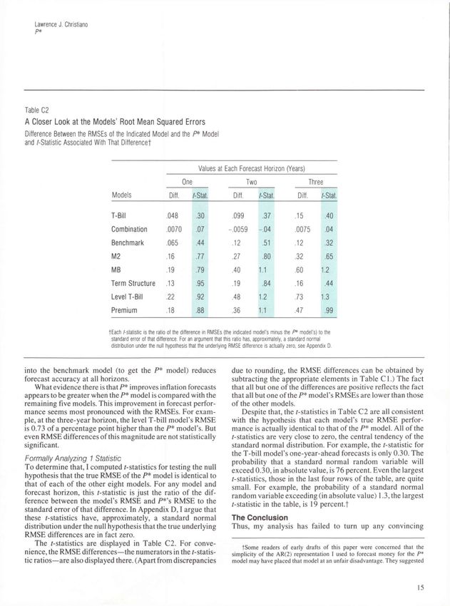
Lawrence J. Christiano
    p*

Charts 6 - 9
. . . A n d Quantitatively
A Comparison of Predicted and Actual Annualized % Changes in the GNP Deflator
Quarterly, 1970:4-1989:3t

                                                    Predicted: _               P * Model               Actual
                                                                  —            T-Bill Model

                       O n e - Y e a r - A h e a d Forecasts                                                               Forecast Errors (Actual - Predicted)

    Chart 6 Inflation Rates                                                                               Chart 8 Two Years Ahead

   1970                 1975                  1980                 1985                                   1970                 1975                  1980   1985

    Chart 7 Inflation Forecast Errors                                                                     Chart 9 Three Years Ahead
            (Actual - Predicted)
% Pts.
 6r

   1970                 1975                  1980                  1985                                  1970                  1975                 1980   1985

   fAII the forecasts begin in 1969:4, but the curves in Charts 8 and 9 start later than the others because these curves are for longer forecast periods
    (two and three years, not just one). Throughout, each forecast is plotted on the last quarter of its period. For example, for the period starting in
    1969:4, the one-year-ahead forecast is plotted at 1970:4; the two-year-ahead forecast, at 1971:4; the three-year-ahead forecast, at 1972:4.
    For technical descriptions of the models, the forecasting procedures, and the forecasts, see Appendixes A, B, and C.
    Sources: Federal Reserve Board of Governors; U.S. Department of Commerce;
               Hallman, Porter, and Small 1989

                                                                                                                                                                   9
does better, then the P* model does better, and finally
the two come together again.
    This same pattern appears in the two- and three-
year-ahead forecast errors, which are plotted in Charts
8 and 9. Overall in these charts, the two models perform
similarly, but there are subperiods in which one domi-
nates the other.
    In sum, neither the P* nor the T-bill model is clearly
much better than the other at forecasting inflation from
one to three years out.8 A comparison of P* and seven
other models (in Appendix C) produces the same result.
If P* is, indeed, the inflation forecaster's holy grail, then
there is little hint of it in the historical data.

                                                                   8
                                                                     For a formal quantitative analysis of the results in Charts 6 - 9 , see
                                                                Appendix C.

10
Lawrence J. Christiano
p*
Appendix A
Describing the P * and T—Bill Models
Here I describe the two competing models in the preceding Board's measure of P* for the calculations reported in the
paper: the P* model and the T-bill model. The P* model is paper. In the table, the coefficients of the P* model seem
relatively insensitive to which measure of P* is used. This is
Att, = a\o g(P?-i/P,-i) + ft A t t ^ + ftA7r,_2 consistent with the results reported in Appendix B, according
to which forecasts from the P* model do not deteriorate when
+ P3A7Tt-3 + j34A7T,_4 + ut my measure of P* is used instead of the Board's.
where Pt is the quarterly price level; nt is the quarterly inflation
rate, defined as irt = log(/J) — log^/J-!); A7i> = n t — 7i>_i;
and u t is the regression error term. The T-bill model is the
same as the above except that \og(P$L\IPt-{) is replaced by
Rt-\ —Rt~2, where Rt is the average of annualized returns for
90-day Treasury bills purchased in quarter t. Both models'
parameters are estimated by the method of ordinary least
squares.
The accompanying table displays estimation results, based
on data covering the period 1960:3-1989:3, for the T-bill
model and two versions of the P* model. The two versions of
the P* model use two different measures of P*: mine and the
Board's. For reasons given in Appendix B, I could not use the
Estimation of Inflation Models
1960:3-1989:3
Values (and Standard Errors) for Each Model
Parameters
and Statistics Board P * My />* T—Bill
a .032 .021 .0012
(.0085) (.0077) (.00042)
ft -.61 -.57 -.59
(.090) (.089) (.092)
ft -.44 -.39 -.40
(.10) (.10) (.10)
ft -.27 -.23 -.27
(.10) (.10) (.10)
ft -.13 -.094 -.13
(.087) (.087) (.090)
Residual S.E. .003960 .003984 .004064
/? 2
.3172 .3087 .2808
11Appendix B
Calculating the Forecasts
Here I describe the calculations underlying Charts 6 - 9 in the
preceding paper. Throughout, forecasts only use data avail- Table B1
able at the date of the forecast. Forecasts computed in this
way are called real-time forecasts. Estimation of Money and Interest Rate Models
Let ^59.4 and P-jq.a denote the price levels in the fourth 1960:3-1989:3
quarters of 1969 and 1970. The actual average inflation rate
between these quarters is log(P 7 o : 4) — log(P69 :4 ). To compute
the forecast of this as of 1969:4, the P* model requires fore- Parameter Values
casts of P*o:i, P*o:2> a n d ^70:3* a n d the T-bill model requires (and Standard Errors)
forecasts of ARt for those periods. Here, A#7 0 : i = R-jo:\ — for Each Modelf
^69:4- Lags on Explanatory
Forecasts of P* require forecasts of V*, the Federal Variable and Statistics M2 AR
Reserve Board's M2 measure of money, and the full capacity
level of output, Q*. Real-time forecasts of V* were computed Zero .012 .0435
using the sample mean of V from 1959:1 until the date of the (.0058) (.082)
forecast. Real-time forecasts of M2 were computed using this
second-order autoregressive [AR(2)] model: One 1.59 .20
(.074) (.089)
(Bl) \og(M2t) = a 0 + «ilo g(M2,_0 Two -.59 -.31
(.074) (.089)
+ a2\og(M2t-2) + et.
Residual S.E. .0064 .88
When estimated over the period 1960:3-1989:3, the param-
eters of this model are as shown in the M2 column of Table R2 .99992 .12
B l . The Box-Pierce Q-statistic and associated significance
0-Stat. at Lag 30 26.82 36.34
level indicate no significant serial correlation in the fitted
residuals. Significance Level .63 .20
Unfortunately, my attempts to construct a real-time ver-
sion of the Federal Reserve Board economists' measure ofLawrence J. Christiano
p*
Table B2 Appendix C
Comparison of Two Versions Analyzing the Forecasts
of the P * Inflation Forecasting Model
Root Mean Squared Errors
Forecast (and Means)
Horizons
(Years) Board P * My P* Here I further analyze the results in Charts 6 - 9 in the pre-
ceding paper, while also describing the results of other tests
One 1.41 1.35 not detailed there. Besides the two models tested in the paper,
(.19) (.020) I also examined the real-time forecasting performance of
seven other models. The results of all the tests are the same:
Two 1.61 1.46 P* is not far superior to other simple methods of forecasting
(.28) (-.0060) inflation.
Three 1.81 1.55
(.45) (.030) 7 More Models and 3 Statistics
Among the seven extra models are two money growth models
Note: The forecast errors underlying these results and one term structure model. In the money growth models,
are out of sample: for each forecast, the I replaced Rt~\ — Rt-2 in the T-bill model (described in
coefficients of the P* model are estimated Appendix A) with log(M2,_ 1 ) — log(M2,_2) and with
using only data available at the time of the
\og(MBt-i) — log(MZ?r_2), where MB is the Federal Reserve
forecast. These forecast errors are not real
time, however, since the forecasts use Board's measure of the monetary base. I used an AR(2) model
actual—not forecasted—values of P*. [equation (B1) in Appendix B] to forecast M2 in the M2 model
and an AR(2) model to forecast MB in the MB model. In the
term structure model, I replaced Rt~\ — Rt-2 in the T-bill
model with R \ 1 — Rt- \, where R\0 is the return on 10-year
Table Bl. Here, too, the Q-statistic and associated signifi- Treasury bonds. To forecast — R in this model, I used an
cance level indicate no significant serial correlation in the AR(2).
residuals. Besides these three models, I also considered four more.
One is the benchmark model mentioned in the paper; it sim-
ply extrapolates inflation from its own past because it sets
a = 0 in the P* model. Another I call combination; it com-
bines the P* and T-bill models in the obvious way, by adding
8(Rt~\ — Rt-2) a s a n explanatory variable to the P* model,
wherethe errors (the MAVE) and the square root of the mean model occurs at the three-year horizon. That improvement is
squared error (the RMSE). The basic difference between these a mere 0.15 of a percentage point, an economically negligible
two is that the RMSE weighs large forecast errors relatively amount in view of the roughly 6 percent inflation we have
more heavily than the MAVE does. All three statistics are averaged over the postwar period. Also, a glance back at
measured in percentage terms at an annual rate. Charts 7 - 9 shows that the magnitude of fluctuations in the
forecast errors is much larger than 0.15 of a percentage point.
The Results This suggests that differences in RMSE of such magnitude are
The results for each model at each forecast horizon are dis-
not statistically significant, or that the superior RMSE
played in Table C1.
performance of the P* model can't be counted on to persist.
Eyeballing the 3 Statistics The formal statistical analysis reported in the next subsection
Consider first the results for the P* and T-bill models, shown supports this conclusion.
in the table's first two rows. They are based on the forecast Bringing the results of the combination and benchmark
errors in the paper's Charts 7 - 9 , and they confirm the paper's models into the analysis offers additional ways to assess how
conclusions: though on some dimensions one model seems to much information about inflation is contained in P*. Thus,
outperform the other, overall the two models perform about comparing the combination and T-bill model results shows
equally well. In terms of bias and average absolute error, the that there is little information in P* that is not already in T-bill
T-bill model outperforms the P* model at all three forecast yield changes. Incorporating P* into the T-bill model (to get
horizons, but in terms of the RMSE, the P* model outperforms the combination model) reduces the bias and magnitude of
the T-bill model at all horizons. In either case, these the T-bill model's forecast errors by a trivial amount.
differences seem too small to be economically or statistically Comparing the benchmark and P* model results suggests a
significant. For example, in RMSE terms, the largest im- sense in which P* actually contains disinformation about
provement from using the P* model rather than the T-bill inflation. According to the mean and MAVE, introducing P*
Table C1
Comparison of Real-Time Performance of Nine Inflation Forecasting Models
Measured by Three Statistics!
(The shaded numbers identify the best model in each column.)
Value of Each Statistic at Each Forecast Horizon (Years)
One Two Three
Models Mean MAVE RMSE Mean MAVE RMSE Mean MAVE RMSE
P*t .38 1.26 1.53 .55 1.46 1.74 .79 1.71 1.98
T-Bill -.12 1.22 1.58 -.26 1.37 1.84 -.39 1.65 2.13
Combination .15 1.18 1.54 .17 1.37 1.73 .24 1.64 1.99
Benchmark -.07 1.25 1.60 -.16 1.38 1.86 -.24 1.64 2.09
M2 -.34 1.30 1.70 -.58 1.44 2.01 -.83 1.72 2.29
MB -.62 1.31 1.72 -1.0 1.60 2.14 -1.5 2.02 2.58
Term Structure .05 1.32 1.67 -.025 1.48 1.93 -.10 1.69 2.14
Level T-Bill -.44 1.30 1.76 -.74 1.55 2.22 -1.1 2.00 2.71
Premium -.32 1.31 1.72 -.54 1.47 2.10 -.76 1.84 2.45
fThe mean is the simple average of the model's forecast errors, the MAVE is the mean of the absolute values of those errors, and the RMSE is the square
root of the mean squared error.
tThe results in this row are based on the version of the P* model that uses my measure of P*, not the Board's. For details on the two versions, see
Appendix B.
14Lawrence J. Christiano
P*
Table C2
A Closer Look at the Models' Root Mean Squared Errors
Difference Between the RMSEs of the Indicated Model and the P* Model
and /-Statistic Associated With That Difference!
Values at Each Forecast Horizon (Years)
One Two Three
Models Diff. /-Stat. Diff. /-Stat. Diff. /-Stat.
T-Bill .048 .30 .099 .37 .15 .40
Combination .0070 .07 -.0059 -.04 .0075 .04
Benchmark .065 .44 .12 .51 .12 .32
M2 .16 .77 .27 .80 .32 .65
MB .19 .79 .40 1.1 .60 1.2
Term Structure .13 .95 .19 .84 .16 .44
Level T-Bill .22 .92 .48 1.2 .73 1.3
Premium .18 .88 .36 1.1 .47 .99
tEach /-statistic is the ratio of the difference in RMSEs (the indicated model's minus the P* model's) to the
standard error of that difference. For an argument that this ratio has, approximately, a standard normal
distribution under the null hypothesis that the underlying RMSE difference is actually zero, see Appendix D.
into the benchmark model (to get the P* model) reduces due to rounding, the RMSE differences can be obtained by
forecast accuracy at all horizons. subtracting the appropriate elements in Table CI.) The fact
What evidence there is that P* improves inflation forecasts that all but one of the differences are positive reflects the fact
appears to be greater when the P* model is compared with the that all but one of the P* model's RMSEs are lower than those
remaining five models. This improvement in forecast perfor- of the other models.
mance seems most pronounced with the RMSEs. For exam- Despite that, the /-statistics in Table C2 are all consistent
ple, at the three-year horizon, the level T-bill model's RMSE with the hypothesis that each model's true RMSE perfor-
is 0.73 of a percentage point higher than the P* model's. But mance is actually identical to that of the P* model. All of the
even RMSE differences of this magnitude are not statistically /-statistics are very close to zero, the central tendency of the
significant. standard normal distribution. For example, the /-statistic for
the T-bill model's one-year-ahead forecasts is only 0.30. The
Formally Analyzing 1 Statistic probability that a standard normal random variable will
To determine that, I computed /-statistics for testing the null exceed 0.30, in absolute value, is 76 percent. Even the largest
hypothesis that the true RMSE of the P* model is identical to /-statistics, those in the last four rows of the table, are quite
that of each of the other eight models. For any model and small. For example, the probability of a standard normal
forecast horizon, this /-statistic is just the ratio of the dif- random variable exceeding (in absolute value) 1.3, the largest
ference between the model's RMSE and P*'s RMSE to the /-statistic in the table, is 19 percent, t
standard error of that difference. In Appendix D, I argue that
these /-statistics have, approximately, a standard normal The Conclusion
distribution under the null hypothesis that the true underlying Thus, my analysis has failed to turn up any convincing
RMSE differences are in fact zero.
The /-statistics are displayed in Table C2. For conve-
fSome readers of early drafts of this paper were concerned that the
nience, the RMSE differences—the numerators in the /-statis- simplicity of the AR(2) representation I used to forecast money for the P*
tic ratios—are also displayed there. (Apart from discrepancies model may have placed that model at an unfair disadvantage. They suggested
15evidence that P* far outperforms other models as an inflation
forecaster. In my tests, P* does worse than its competitors on
some dimensions and better on others. The dimension on
Appendix D
which P* looks best is the estimated RMSE of its forecast Rationalizing the Use
errors. But the superiority of P* on this dimension is so small
that it could just reflect dumb luck.
of the Standard Normal Distribution
Here I explain why the r-statistics in Appendix C's Table C2
can be interpreted as though they were drawn from the
standard normal distribution.
An Approximation
Let 7 denote the estimator underlying the numbers in any of
the differences columns in that table. Thus, 7 is the estimated
RMSE for the forecasts of one of the models in the table minus
the corresponding RMSE for the forecasts of the P* model.
Let 7 denote the underlying true RMSE difference. This is
what 7 would be if it were computed using an unlimited
number of observations instead of the 70-odd data points that
are actually available. I use Hansen's (1982) generalized
method of moments formula to estimate the standard error of
7 . To a first approximation, the ratio of 7 to this standard
error (the r-statistic discussed in Appendix C) has an asymp-
totic standard normal distribution under the null hypothesis
that 7 is zero.
To use Hansen's standard error formula, I must express 7
as the solution to the sample analog of some first-moment
condition. To keep the notation simple, I describe here just the
calculations for the T-bill model's one-year-ahead forecast
errors. The calculations for all the other models and forecast
horizons are analogous.
To start, define this 2 X 1 random variable:
(Dl) ht(y,o) = {7(7 + 2a] - e(AR,t)2 + e(P*,0 2 ,
o2-e(P*,t)2}'
where a is the RMSE for the P* model's forecasts and e(AR,t)
and e(P*,t) are the date t one-year-ahead forecast errors
from the T-bill and P* models. Also, 7 = or — a, where or is
the RMSE for the T-bill model's forecasts, so that 717 + 2o]
= o\ — o2. Therefore, if a is the (unknown) true value of a,
then Eht(7, a) = 0 for each t. This is the first-moment
condition that underlies my estimator of 7 (and a).
an alternative procedure which avoids the need to forecast other variables when The sample analog of this condition is
forecasting inflation: use annual or biennial rather than quarterly observations
to forecast inflation one or two years out. Note that, effectively, this procedure (D2) gT(y,o) = {y[y + 2a]
throws away a large number of observations. Other things the same, one expects
that to result in a deterioration in forecast performance. Still, to investigate this - (l/T)Xj={[e(ARtt)2 - e(P*,t)2],
suggestion, I used annual data to compute a set of real-time, one-year-ahead
forecast errors using annual versions of my P*, T-bill, combination, and a2-(l/r)2f=1e(PV)2}'.
benchmark models. I found that the forecast performance of all these models is
generally inferior to that of their quarterly counterparts. Moreover, the annual
P* model forecasts less well than all of my quarterly models: the quarterly T-bill Here T is the number of observations used in the RMSE
and benchmark models beat it in terms of all three of my statistics, and the other calculations (76, 72, and 68 for the one-, two-, and three-
quarterly models beat it in terms of two of the three, the mean and the MAVE. year-ahead forecast errors). It is easy to confirm that my
16Lawrence J. Christiano
P*
estimators of y and o (the 7 defined above and the estimated about the comparable RMSE performance of the P* and
RMSE of the P* model's forecast errors) uniquely satisfy T-bill models, for example, would require showing that my
gr( yfi) = 0. /-statistics are biased downward by a factor of at least five.
Now define This is because the largest of those /-statistics is 0.4 and
rejecting a null hypothesis at the conventional 5 percent sig-
(D3) DT= dgT(y,o)/d(y,o) nificance level requires a /-statistic roughly equal to 2.
evaluated at 7 = 7 and o = a. Hansen (1982) shows that if
h t (7,a) is strictly stationary and other regularity conditions
are satisfied, then for large T
(D4) ^ \ J is normally distributed with mean £ T J and
variance V
where Vis a positive definite matrix consistently estimated by
(D5) V = (Dj)~1S(Df 1 / T.
Here S is a matrix that I will explain in the next paragraph.
Meanwhile, we can already see by (D4) and (D5) that the
estimated standard error of 7 is the square root of the first
diagonal element of V. (The square root of the second
diagonal element is Hansen's estimator of the standard error
of a.) For the T-bill model's one-year-ahead forecast errors,
the standard error of 7 is 0.16, thus accounting for the 0.30
/-statistic in Table C2. (The standard errors of 0 at the one-,
two-, and three-year-ahead horizons are 0.18, 0.20, and
0.40.)
To return to S in (D5): It is a consistent estimator of 5, the
spectral density at frequency zero of h t (y,5). In particular,
(D6) 5= X~=-ooE{ht(y,8)[ht-k(y,d)Y}.
Both S and S are 2 X 2 matrices, and S is assumed to be
positive definite under the regularity conditions. My estimator
of S, 5, replaces the population second moments on the right
side of (D6) by their sample counterparts and truncates the
summation for \k\ > 6 . In addition, I linearly damp higher-
order covariances according to the formula of Doan (1988,
p. 14-143) with 6 = 1.
A Hitch?
An attractive feature of Hansen's estimator of the variance-
covariance of ( 7 , 5 ) is that it is robust to autocorrelation and
conditional heteroscedasticity in ht(7,a). However, as Chris-
topher Sims has pointed out to me, Hansen's stationarity
requirement may not be satisfied. After all, model parameter
estimates are based on less data at the beginning of a sample
period than at the end. Therefore, forecast errors may have
larger variance at the beginning than at the end.
Charts 7 - 9 in the paper give (slight) support for this
possibility. Thus, it may be worthwhile to investigate whether
failure of Hansen's stationarity assumption substantially af-
fects my standard error estimates. Still, I suspect that it does
not, for my results are very strong. To overturn my conclusion
17References
Barro, Robert J. 1987. Macroeconomics. 2nd ed. New York: Wiley.
Business/Economics focus. 1989. Star gazing. Economist 312 (July 15-21): 65.
Christiano, Lawrence J., and Eichenbaum, Martin. 1989. Unit roots in real
GNP: Do we know, and do we care? Working Paper 3130. National
Bureau of Economic Research. Also, forthcoming in Carnegie-Rochester
Conference Series on Public Policy 32. Amsterdam: North-Holland.
Cochrane, John H. 1988. How big is the random walk in GNP? Journal of
Political Economy 96 (October): 893-920.
Doan, Thomas A. 1988. User's manual: RATS (Regression analysis of time
series). Version 3.00. Evanston, 111.: VAR Econometrics.
Dwyer, Gerald P., Jr., and Hafer, R. W. 1988. Is money irrelevant? Review
(May/June): 3 - 1 7 . Federal Reserve Bank of St. Louis.
Fisher, Irving. 1911. The purchasing power of money. New York: Macmillan.
Hallman, Jeffrey J.; Porter, Richard D.; and Small, David H. 1989. M2 per unit
of potential GNP as an anchor for the price level. Staff Study 157. Board
of Governors of the Federal Reserve System.
Hansen, Lars Peter. 1982. Large sample properties of generalized method of
moments estimators. Econometrica 50 (July): 1029-54.
Heinemann, H. Erich. 1989. Overview/Commentary: Cure for Greenspan's
dilemma is not to be found in formula. American Banker 154 (June 19):
4, 8.
Hunt, Lacy H. 1989. Forecasting inflation: The Fed's new tool just doesn't
work. New York Times 138 (October 22): Business 2.
Kilborn, Peter T. 1989. Federal Reserve sees a way to gauge long-run inflation.
New York Times 138 (June 13): 1.
Lee, L. Douglas. 1989. 'P-Star' can spot inflationary trends. New York Times
138 (October 22): Business 2.
Lucas, Robert E., Jr. 1980. Two illustrations of the quantity theory of money.
American Economic Review 70 (December): 1005-14.
. 1986. Adaptive behavior and economic theory. Journal of
Business 59 (Part 2, October): S401-26.
McNamee, Mike. 1989. Putting 'Keynes's head on Milton Friedman's body.'
Business Week (July 31): 66.
Nelson, Charles R., and Plosser, Charles I. 1982. Trends and random walks in
macroeconomic time series: Some evidence and implications. Journal of
Monetary Economics 10 (September): 139-62.
Sims, Christopher A. 1989. Modeling trends. Discussion Paper 22. Institute for
Empirical Macroeconomics (Federal Reserve Bank of Minneapolis and
University of Minnesota).
Walter, John R. 1989. Monetary aggregates: A user's guide. Economic Review
75 (January/February): 20-28. Federal Reserve Bank of Richmond.
18You can also read