Implementation of a roughness sublayer parameterization in the Weather Research and Forecasting model (WRF version 3.7.1) and its evaluation for ...
←
→
Page content transcription
If your browser does not render page correctly, please read the page content below
Geosci. Model Dev., 13, 521–536, 2020
https://doi.org/10.5194/gmd-13-521-2020
© Author(s) 2020. This work is distributed under
the Creative Commons Attribution 4.0 License.

Implementation of a roughness sublayer parameterization
in the Weather Research and Forecasting model (WRF
version 3.7.1) and its evaluation for regional climate simulations
Junhong Lee1,a , Jinkyu Hong1 , Yign Noh1 , and Pedro A. Jiménez2
1 Department    of Atmospheric Sciences, Yonsei University, Seoul, Republic of Korea
2 Research  Application Laboratory, National Center for Atmospheric Research, Boulder, CO, USA
a current affiliation: Max Planck Institute for Meteorology, Hamburg, Germany

Correspondence: Jinkyu Hong (jhong@yonsei.ac.kr)

Received: 26 August 2019 – Discussion started: 2 October 2019
Revised: 21 December 2019 – Accepted: 13 January 2020 – Published: 11 February 2020

Abstract. The roughness sublayer (RSL) is one compart-           1   Introduction
ment of the surface layer (SL) where turbulence deviates
from Monin–Obukhov similarity theory. As the computing           The planetary boundary layer (PBL) is important for the
power increases, model grid sizes approach the gray zone         proper simulation of weather, climate, wind energy applica-
of turbulence in the energy-containing range and the lowest      tion, and air pollution. Turbulence plays a critical role in the
model layer is located within the RSL. From this perspective,    spatiotemporal variation of the PBL structure through the tur-
the RSL has an important implication in atmospheric model-       bulent exchanges of momentum, energy, and water between
ing research. However, it has not been explicitly simulated in   the atmosphere and Earth’s surface. Because turbulent eddies
atmospheric mesoscale models. This study incorporates the        in the PBL are smaller than the typical grid size in mesoscale
RSL model proposed by Harman and Finnigan (2007, 2008)           and global models, their impacts must be properly parame-
into the Jiménez et al. (2012) SL scheme. A high-resolution      terized for atmospheric models. The surface layer (SL) oc-
simulation performed with the Weather Research and Fore-         cupies the lowest 10 % of the PBL where the shear-driven
casting model (WRF) illustrates the impacts of the RSL pa-       turbulence is dominant. In the SL, Monin–Obukhov similar-
rameterization on the wind, air temperature, and rainfall sim-   ity theory (MOST), which is a zero-order turbulence closure,
ulation in the atmospheric boundary layer. As the roughness      provides the relationships between the vertical distribution
parameters vary with the atmospheric stability and vegeta-       of wind and scalars and the corresponding fluxes in a given
tive phenology in the RSL model, our RSL implementation          stability condition (Obukhov, 1946; Monin and Obukhov,
reproduces the observed surface wind, particularly over tall     1954). The typical numerical weather prediction (NWP) and
canopies in the winter season by reducing the root mean          climate models are applied for the SL parameterization based
square error (RMSE) from 3.1 to 1.8 m s−1 . Moreover, the        on MOST to parameterize the subgrid-scale influences of the
improvement is relevant to air temperature (from 2.74 to         turbulent eddies in the PBL (e.g., Sellers et al., 1986, 1996).
2.67 K of RMSE) and precipitation (from 140 to 135 mm per           The SL has two parts: the inertial sublayer (ISL) and the
month of RMSE). Our findings suggest that the RSL must           roughness sublayer (RSL). The ISL is the upper part of
be properly considered both for better weather and climate       the SL, where MOST is valid and vertical variation of the
simulations and for the application of wind energy and atmo-     turbulent fluxes is negligible. The RSL is the layer near and
spheric dispersion.                                              within the surface roughness elements (e.g., trees and build-
                                                                 ings). The turbulent transport in the RSL has a mixing layer
                                                                 analogy, and the atmospheric flow depends on the rough-
                                                                 ness element properties (Raupach et al., 1996). Accordingly,
                                                                 the flux–gradient relationships in the RSL deviate from the

Published by Copernicus Publications on behalf of the European Geosciences Union.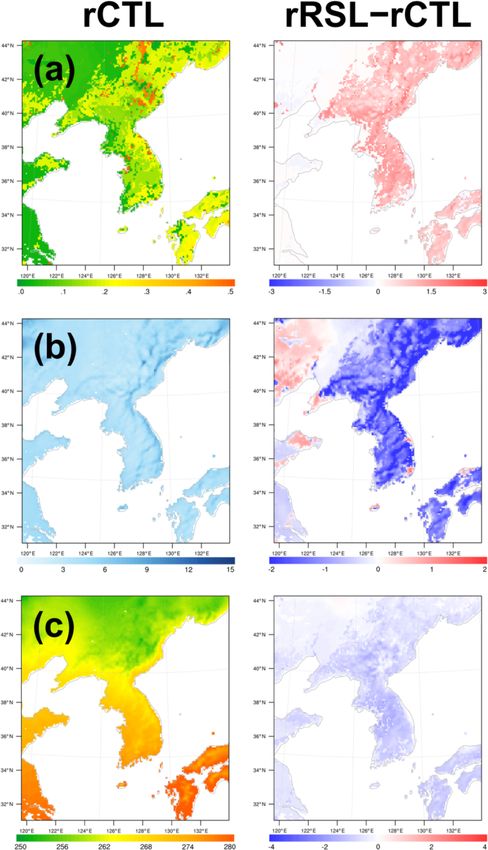
522 J. Lee et al.: Implementation of a roughness sublayer parameterization in the WRF version 3.7.1 model
MOST predictions, and the eddy diffusion coefficients are tion of the HFs into the WRF model (version 3.7.1). For this
larger than the values in the ISL (e.g., Shaw et al., 1988; purpose, we reformulate the HFs’ RSL parameterization to
Kaimal and Finnigan, 1994; Brunet and Irvine, 2000; Finni- implement it in the SL parameterization in the WRF model
gan, 2000; Hong et al., 2002; Dupont and Patton, 2012; Shap- and then discuss the impacts of the RSL parameterization on
kalijevski et al., 2016; Zhan et al., 2016; Basu and Lacser, the regional weather and climate simulations in terms of me-
2017). teorological conditions near the Earth’s surface. To the best
Traditionally, the RSL has not been explicitly considered of the authors’ knowledge, our study is the first extensive at-
in global and mesoscale models because the PBL in the tempt to incorporate the RSL parameterization into the WRF
model is coarsely resolved, and the lowest model layer is model and to validate it for regional climate simulations. Sec-
well above the roughness elements accordingly. As the com- tion 2 presents a brief discussion of the RSL parameteriza-
puting power increases, the grid size of the NWP model de- tion of HFs and the implementation procedures into the WRF
creases and it gets close to the grid size of gray zone for the model. Section 3 explains the experimental and observational
turbulence. Nevertheless, studies on the impact of a fine ver- descriptions. Section 4 presents the impacts of the RSL pa-
tical resolution have not been relatively performed. From this rameterization. Section 5 ends the study with the concluding
perspective, the RSL has an important implication in atmo- remarks.
spheric modeling research. The lowest model layer is typ-
ically approximately 30 m high, and its vertical resolution
continues to be better; hence, the models have more than 2 RSL theory of the HFs
one vertical layer in the RSL, which extends to 2–3 times
The roughness sublayer parameterization by HFs is adopted
the canopy height. Furthermore, model outputs are sensitive
herein along with an explanation of the core of HFs’ model,
to the selection of the lowest model level height (Shin et al.,
and the relevant details on this parameterization can be found
2012), but its relation to the RSL has not yet been clearly in-
in Harman and Finnigan (2007, 2008) and Harman (2012).
vestigated. Accordingly, turbulent transport in the RSL must
Appendix A lists the symbols and variables used in this study
be incorporated particularly in the mesoscale models if the
in alphabetical order.
vertical model levels are inside the RSL with an increase in
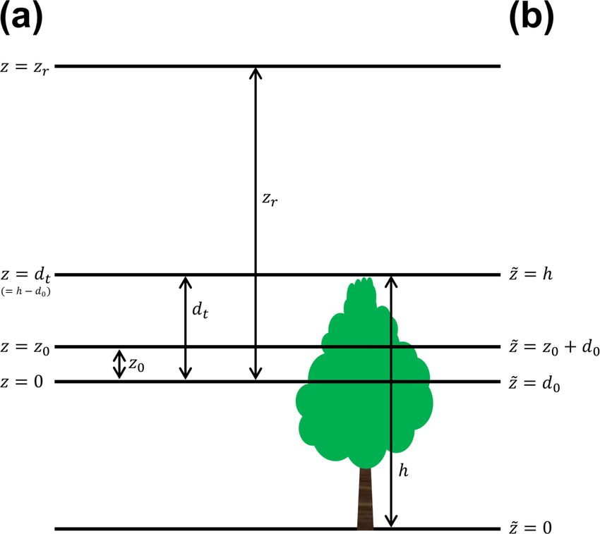
We first define the coordinate alignment for its applica-
the vertical model resolution.
tion to the WRF. The revised MM5 SL scheme in the WRF
The RSL function is a popular and simple method of incor-
model defines the vertical origin by the conventional zero-
porating the effects of the RSL in the observation and model
plane displacement height (d0 ). The same coordinate system
(e.g., Raupach, 1992; Physick and Garratt, 1995; Wenzel et
is also applied herein. The vertical coordinates z and z̃ in this
al., 1997; Mölder et al., 1999; Harman and Finnigan, 2007,
coordinate system are defined as the distance from d0 and
2008; de Ridder, 2010; Arnqvist and Bergström, 2015). The
from the terrain surface, respectively; therefore, their relation
RSL function is defined as the observed relationship between
is z = z̃ − d0 (Fig. 1). Note that a vertical origin in the HFs
the vertical gradient of wind and scalar variables and their
is at the canopy height (h). MOST says that a variable (C),
corresponding fluxes in the RSL. Accordingly, simple rela-
such as wind speed (u) and temperature (T ), has the follow-
tionships are appropriate for the land surface model in the cli-
ing logarithmic vertical profile:
mate model and for the mesoscale model (Physick and Gar-
ratt, 1995; Sellers et al., 1986, 1996). Despite the importance k
z z z
0
of the RSL, the Weather and Research Forecasting (WRF) (C(z) − C0 ) = ln − ψc + ψc , (1)
C∗ z0 L L
model (Skamarock et al., 2008), which is one of the widely
used models in the operation and research fields, does not where k is von Kármán constant; C∗ is a C scale; C0 is C
consider the effects of the RSL for the regional weather and at z0 ; z0 is the roughness length; ψc is the integrated similar-
climate simulations. Harman and Finnigan (2007, 2008) and ity function of C; and L is the Obukhov length. The C profile
Harman (2012) (hereafter, HFs) recently proposed a rela- based on the RSL function of the HFs is divided into two lay-
tively simpler RSL function that can be used in a wide range ers depending on the relative distance between the canopy
of atmospheric models. The RSL function of the HFs is based height and the redefined zero-plane displacement height in
on a theoretical background and applicable to a wide range the HFs (dt = h−d0 ): the upper-canopy layer (z > dt ), where
of atmospheric stabilities by succinctly satisfying the conti- the influence of additional mixing by the canopy exists, and
nuity of the vertical profiles of fluxes, wind, and scalars both the lower-canopy layer (z < dt ), where the canopy is the di-
at the top of the RSL and at the top of a canopy. The pa- rect source and sink for drag and heat (Fig. 1). The vertical
rameterization of HFs has recently been incorporated in a profile in the upper-canopy layer is described as follows:
one-dimensional (1-D) PBL model and a land surface model
(Harman, 2012; Shapkalijevski et al., 2017; Bonan et al.,
2018).
Based on the abovementioned background, this study in-
corporates the RSL parameterization based on the RSL func-
Geosci. Model Dev., 13, 521–536, 2020 www.geosci-model-dev.net/13/521/2020/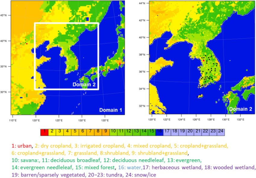
J. Lee et al.: Implementation of a roughness sublayer parameterization in the WRF version 3.7.1 model 523
k z z z
0
(C(z) − C0 ) = ln − ψc + ψc
C∗ z0 L L
Z∞ φc 1 − φ̂c
+ dz0 , (2)
z0
z
where φc is the similarity function of C, and φ̂c is an RSL
function of C. In the z → ∞ limit, φ̂c is equal to 1 and
the wind speed converges to the MOST prediction. The last
term on the right-hand side represents the additional mixing
caused by the roughness element due to the coherent canopy
turbulence and can be replaced by ψ̂c , which is an integrated
RSL function of C. The vertical profile from the HFs for the
RSL deviates from that of MOST because of ψ̂c , thereby ad-
justing the logarithmic profile. The φ̂c is introduced as fol-
lows:
β Figure 1. The schematic diagram to describe the vertical coordi-
φ̂c = 1 − c1 exp −c2 z . (3) nate systems used in this study. (a) The vertical coordinate of the
lm
Yonsei University surface layer (YSL) schemes (z) is defined as the
distance from the conventional zero-plane displacement height (d0 )
c1 and c2 are then determined from the continuity of φ̂c at
and (b) the convectional coordinate (z̃) is defined as the distance
the canopy top, and the RSL function, φ̂c , exponentially con- from terrain surface. Here, z0 , dt , h, and zr are roughness length,
verges to zero above the RSL. In the lower canopy layer, the redefined zero-plane displacement height in Harman and Finni-
C has the following exponential form: gan (2007), canopy height, and the lowest model layer in the con-
ventional coordinate, respectively.
z − dt
C(z) − C0 = (Ch − C0 ) exp f . (4)
2dt
3 Incorporation of the roughness sublayer
The RSL functions vary with atmospheric stability parameterization into the WRF model
through β:
The RSL parameterization of the HFs described above is im-
βN Lc
> −0.15 plemented in the Jiménez et al. (2012) revised MM5 sur-
φm (z=dt ) L
β=
βN k
, (5) face layer scheme and Noah land surface model in the WRF
k φm (z=dt ) − 2φm (z=dt ) Lc
2φm (z=dt ) + 1.5 L ≤ −0.15 (hereafter called the Yonsei University surface layer (YSL)
1+2 LLc +0.15
scheme) because of theoretical consistency between the HFs
and PBL parameterization. To incorporate the RSL parame-
where Lc is a canopy penetration depth defined as
terization, it is necessary to modify the SL scheme as follows
4h (Fig. 2): the first step is to compute the bulk Richardson num-
Lc = (cd a)−1 = , (6) ber at the lowest model layer, Bib , by the original equation
LAI
of Jiménez et al. (2012) (Eq. 9 in their study):
where cd is a drag coefficient at the leaf scale and a is the
g θva − θvg
leaf area density. The parameters dt and z0 also depend on Bib = z. (9)
the stability because of their dependence on β: θa [u (zr )]2
The second step is to iteratively calculate the atmospheric
lm
dt = h − d0 = = β 2 Lc , (7) stability (zr /L) as follows with an accuracy of 0.01:
2β
z h i2
k dt 0 ln zz0r − ψm zLr + ψm zL0 + ψ̂m
z0 =dt exp − exp −ψm + ψm zr
β L L = Bib , (10)
L ρcp kun−1
∗ zr zr zr zl
ln cs + zl − ψ h L + ψh L + ψ̂h
Z∞ φm 1 − φ̂m
exp dz0 . (8)
z0 where un−1
∗ is the friction velocity (u∗ ) at the previous time
dt step. Equation (10) is different from Eq. (23) of Jiménez et
al. (2012) by the RSL functions (i.e., ψ̂m and ψ̂h ). After zr /L
www.geosci-model-dev.net/13/521/2020/ Geosci. Model Dev., 13, 521–536, 2020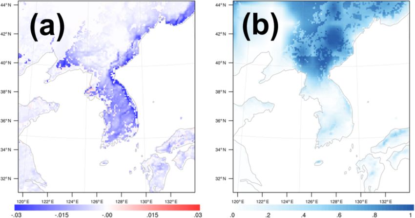
524                   J. Lee et al.: Implementation of a roughness sublayer parameterization in the WRF version 3.7.1 model

is determined, the third step is to iteratively update dt and β
using Eqs. (5) and (7) with an accuracy of 0.0001 because
they are intercorrelated with each other. Subsequently, z0 is
iteratively achieved with an accuracy of 0.0001 using Eq. (8)
at the given zr /L, β, and dt . The u profile is determined using
Eqs. (2) and (4). Following Jiménez et al. (2012), the profile
of a scalar, such as T , is determined by
                                              !
  k                       ρcp kun−1
                                 ∗ zr      zr         z
     (C(z) − C0 ) = ln                  +       − ψc
C∗                              cs         zl            L

                         z  Z∞ φc 1 − φ̂c
                            0
                  + ψc          +                  dz0 ,     (11)
                           L              z0
                                              z
for the upper-canopy layer. Equation (4) is used for the lower-
canopy layer. Finally, u∗ is given to
                             ku (zr )
u∗ = h                                                    i,         (12)
                                                  z0
      ln zz0r − ψm            zr
                              L + ψm              L + ψ̂m

and the aerodynamic conductance from z = 0 to z = zr (ga )
in the RSL is given to
         Zzr
                dz
1/ga =                ≡ 1/ga1 + 1/ga2 + 1/ga3                          (13)
               Kh (z)                                                          Figure 2. Flow diagram of the RSL parameterization. The gray
         0                                                                     boxes indicate the iteration module.
          Zzl          Zzl
             dz                 dz
1/ga1 ≡             =               cs
            Kh (z)         ku∗ z + ρc                                          Table 1. Idealized boundary condition for the one-dimensional of-
                                      p
        0              0                                                       fline simulation. Constant z0 is used only in the CTL experiment.

          1        ku∗ zl
      =      ln            +1                                          (14)     Variable             Value              Variable   Value
        ku∗       cs /ρcp
          Zdt                                                               h                    18 m               Sm         0.25 m3 m−3
                 dz     Sc         dt − zl                                      LAI                  4 m2 m−2           T (zr )    300 K
1/ga2 =               = 2    exp β           −1 ,                      (15)
                Kh (z) β uh           lm                                        Land-use category    Mixed forest       Tsk        303 K
          zl                                                                    Lc                   18 m               u(zr )     3 m s−1
          Zzr                Zzr                                             p(zr )               1000 hPa           u∗         0.5 m s−1
                 dz                 8h         1      zr                        q(zr )               9.3 × 10 kg kg−3   z/L        −10 to 10
1/ga3 =                =                 dz =      ln
                Kh (z)             ku∗ z      ku∗     dt                        SW                   800 W m−2          z0         0.25 m
          dt                 dt
               z
                 r                dt               zr           dt
      −ψh             + ψh                 + ψ̂h β      − ψ̂h β       . (16)
                L                 L                lm           lm
                                                                               without the RSL parameterization, respectively, and were
Computing time increased only 8 % with 61 vertical layers in
                                                                               driven by the idealized forcing data described in Table 1.
the YSL scheme despite more iterations in the YSL scheme
                                                                               The real case simulation consisted of two experiments: re-
compared to the revised MM5 SL scheme.
                                                                               producing 1 month of winter (January 2016) with the revised
                                                                               MM5 SL scheme and the YSL scheme (hereafter referred
4   Numerical experimental design                                              to as the rCTL and rRSL experiments). The rCTL and the
                                                                               rRSL employed the same physics package, except for the
This study evaluated the YSL scheme by making a 1-D of-                        SL scheme and the land surface model (Lee and Hong, 2016
fline and real case simulations. The 1-D offline simulations                   and references therein). One-way nesting was applied herein
were done to test the YSL scheme performance without feed-                     in a single-nested domain with a Lambert conformal map
back with the atmosphere. The 1-D offline simulation con-                      projection to east Asia (Fig. 3). A 9 km horizontal resolu-
sisted of the YSL and the revised MM5 SL schemes cou-                          tion domain 2 was then embedded in the 27 km resolution
pled with the Noah land surface model (i.e., offCTL and of-                    domain 1 with 61 vertical layers. The initial and boundary
fRSL experiments) (Table 1). In the offline simulations, of-                   conditions were produced using the National Center for En-
fCTL and offRSL indicate numerical experiments with and                        vironmental Prediction Final Analysis data (1◦ × 1◦ ).

Geosci. Model Dev., 13, 521–536, 2020                                                               www.geosci-model-dev.net/13/521/2020/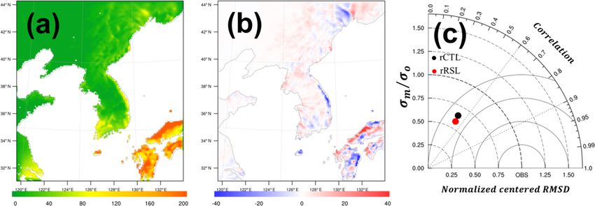
J. Lee et al.: Implementation of a roughness sublayer parameterization in the WRF version 3.7.1 model                              525

Figure 3. Domains and land-use category (USGS) of the real case simulation. Black circles denote the automatic synoptic observing system
in South Korea used for the model evaluation.

5   Observation data for the model evaluation                         6     Results

The model performance was examined against the surface                6.1    Offline simulations
wind speed, surface temperature and precipitation observed
at 46 Automated Synoptic Observing System (ASOS) sites in
                                                                      Figure 4 shows the roughness parameters (i.e., z0 , dt , and β)
South Korea (Fig. 3). Quality control of the data includes gap
                                                                      as a function of the normalized atmospheric stability (Lc /L)
detection, a limit test, and a step test based on the standard of
                                                                      from the 1-D offline simulation of the YSL scheme (of-
the World Meteorological Administration and Korea Meteo-
                                                                      fRSL). The offline YSL simulations reproduced the results
rological Administration (KMA) (Zahumenský, 2004; Hong
                                                                      of HFs. The roughness parameters varied with the atmo-
et al., 2019). For the model evaluation of the real case simu-
                                                                      spheric stability, Lc /L, and had peaks at weakly unstable
lation, the three different measures of the correlation coeffi-
                                                                      conditions. These dependencies of the roughness parameters
cients, centered root mean square differences (RSMDs), and
                                                                      on the atmospheric stability are distinct from typical manner
standard deviations of the model (σm ) normalized by that of
                                                                      of dealing with the roughness parameters as a constant in at-
the observation (σo ) are together shown in a Taylor diagram
                                                                      mospheric models. The roughness length is indeed constant
(Taylor, 2001). In the Taylor diagram, a point nearer the ob-
                                                                      based on the land cover in all the SL schemes in the WRF.
servation at a reference point (OBS) can be considered to
                                                                         Figure 5 indicates that the impacts of the RSL are
give a better agreement with the observation. We also pro-
                                                                      also a function of Lc , which is a function of LAI and h
vide the root mean square error (RMSE) and the mean bias
                                                                      (Eq. 6), thus leading to both diurnal and seasonal variation
(MB) with the pattern correlation for the rainfall simulation
                                                                      of canopy roughness. Consequently, the roughness parame-
evaluation.
                                                                      ters showed daily and seasonal variations. Overall, the rough-
                                                                      ness length in the YSL was larger than that in the revised
                                                                      MM5 SL scheme, particularly in a smaller z/L (i.e., neu-
                                                                      tral and unstable conditions) and a larger Lc (i.e., small LAI
                                                                      and/or large h). The roughness length in a stable condition
                                                                      showed relatively smaller changes with z/L and Lc com-
                                                                      pared to those in the unstable condition. Our findings suggest
                                                                      that a small LAI in the winter season makes a larger Lc be-

www.geosci-model-dev.net/13/521/2020/                                                       Geosci. Model Dev., 13, 521–536, 2020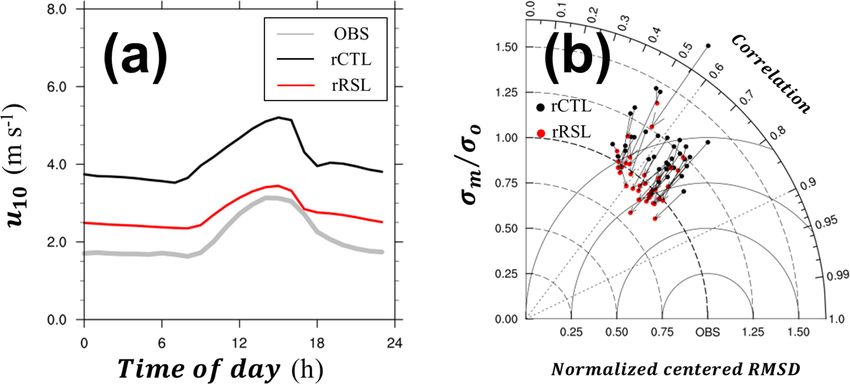
526              J. Lee et al.: Implementation of a roughness sublayer parameterization in the WRF version 3.7.1 model

Figure 4. Roughness length (a), redefined displacement height (b) and β (c) at a given normalized stability (Lc /L) from the offRSL simu-
lation with the YSL scheme. Roughness length and redefined displacement height are normalized by their values in a neutral condition (z0N
and dtN ), respectively.

                                                                       file (i.e., φ̂c → 1) as z increases with the continuous vertical
                                                                       profiles of the wind and the temperature. The YSL scheme
                                                                       reproduced these properties of φ̂c and matched with the ob-
                                                                       served profiles inside canopies: the YSL scheme showed ex-
                                                                       ponential profiles under the canopy top and logarithmic pro-
                                                                       files above the canopy top (Fig. 6). The wind speed and the
                                                                       air temperature above the canopy top were smaller than pre-
                                                                       dicted by MOST because φ̂c < 1 in the offRSL experiments.
                                                                       Furthermore, the YSL scheme produced wind and tempera-
                                                                       ture within the canopy (i.e., z̃ < z0 + d0 ), thereby providing
                                                                       additional useful information on the atmospheric dispersion
                                                                       inside the canopy.
                                                                          The roughness length changes in the YSL scheme eventu-
                                                                       ally produced changes in the surface energy balance with the
                                                                       atmospheric stability (Fig. 7). In the 1-D offline simulations
                                                                       based on the conditions in Table 1, the YSL scheme produced
Figure 5. Roughness length difference (m) between offCTL and
                                                                       a larger z0 in the unstable and near-neutral conditions but a
offRSL (offRSL–offCTL) at given atmospheric stability (z/L) and
penetration depth (Lc ).                                               smaller z0 in z/L > 3 compared to the offCTL. The aerody-
                                                                       namic conductance (ga ) in the YSL scheme was larger in all
                                                                       the stability conditions, even in the stable conditions in which
cause of the smaller LAI, thereby leading to relatively larger         the YSL provided a smaller z0 because the additional term in
differences of z0 between the YSL scheme and the default               Eq. (13), ga2 , dominated over the other effects in the ga cal-
WRF scheme. On the contrary, a similar value of z0 was ob-             culation. Accordingly, H and λE in the YSL scheme were
served in summer because of the larger LAI. Note that the              larger than those in the revised MM5 SL scheme. Our find-
revised MM5 SL scheme does not consider dt and β.                      ing implies stronger fluxes from the YSL scheme when the
   The RSL function, φ̂c , was introduced to consider the ad-          gradient of quantity is the same. However, the impact of the
ditional mixing caused by the roughness element. Accord-               increased ga was asymmetrical in H and λE depending on
ingly, φ̂c should asymptotically converge to the MOST pro-             the soil moisture content. In this case simulation, an increase

Geosci. Model Dev., 13, 521–536, 2020                                                      www.geosci-model-dev.net/13/521/2020/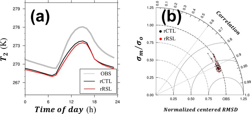
J. Lee et al.: Implementation of a roughness sublayer parameterization in the WRF version 3.7.1 model                                    527

Figure 6. (a) Profiles of the RSL function for momentum (φ̂m , solid line) and heat (φ̂h , dashed line), (b) wind speed (m s−1 ), and (c) tem-
perature (K) at a neutral condition from offCTL (black) and offRSL (gray). The height of conventional coordinate system (z̃) is normalized
by the canopy height (h).

in λE was dominant because the wet condition made more                   the better observed diurnal variation by reducing the positive
partitioning of the available energy into the latent heat flux           bias of the wind speed (Table 2, Fig. 9). Over the tall for-
first in the model. However, in the dry condition (i.e., less            est canopies, u10 in the rRSL was reduced by approximately
soil water content), the YSL produced a larger H without a               30 %; however, the region of the increased wind speed cor-
substantial increase of λE (Fig. S1 in the Supplement). A                responded to the short canopies, where the roughness length
significant increase in λE was found along with a decrease               increased (Fig. 8a and b). The YSL scheme particularly pro-
in H in the strong unstable conditions (Fig. 7) because of               vided a better RMSD and correlation coefficient but less di-
the wet soil moisture of 0.25 m3 m−3 in the offRSL simula-               urnal variability of wind speed because of a relatively larger
tion in Table 1. The slight increase in the net radiation was            reduction of the daytime wind speed (Fig. 9). MB and RMSE
mainly associated with the reduced outgoing longwave radia-              decreased from 2.4 to 1.0 m −1 and from 3.1 and 1.8 m s−1 .
tion caused by the smaller surface temperature in the offRSL.            The Taylor diagram shows that the overall performance of
                                                                         the YSL scheme is better than the default WRF simulation at
6.2   Real case simulations                                              all the 46 sites. In the Taylor diagram, the statistics moved to-
                                                                         ward the observation, except for one site, indicating an over-
Figure 8 shows the real case simulation of the roughness                 all improvement of 2 m air temperature in the YSL scheme;
length, 10 m wind speed (u10 ), and 2 m air temperature (T2 ).           however, the impact of the RSL was not as large as the wind
We discuss herein the real cases in the winter season be-                speed (Table 2, Fig. 10).
cause of stronger effect of the roughness sublayer. The re-                 Similar to the increases of the aerodynamic conductance in
sults for the summer season can be found in the Supple-                  the offline simulations, the YSL scheme in the real case simu-
ment. The roughness length in the rCTL experiment was pre-               lation (i.e., the rRSL simulation) simulated a larger ga , partic-
scribed from the vegetation data table (i.e., VEGPARM table              ularly in the forest canopies and mountain regions (Fig. 11a).
in the WRF model) and modified by the vegetation fraction                This larger ga in the YSL scheme led to the increases of the
(Fig. 8a).                                                               latent heat fluxes by approximately 20 W m−2 , with an even-
   Overall, the YSL scheme (rRSL experiment) produced                    tual reduction of the soil water content (Fig. 12a). The sen-
0.2–2.0 m larger z0 than the default values in the rCTL ex-              sible heat fluxes in the rCTL experiments were generally ap-
periment over the tall canopies, where Lc was large. In con-             proximately 80 W m−2 , except over the snow-covered region
trast, the YSL scheme produced a similar or even slightly                where H was approximately 40 W m−2 . As described in the
smaller z0 over the short canopies compared to the rCTL                  offline simulation, the changing sign of H in the rRSL de-
experiment. Importantly, the changes of z0 made direct im-               pended on the soil moisture content because evapotranspira-
pacts on the momentum fluxes and thus surface wind speed                 tion is limited in dry soils at given available energy (Figs. 11b
(Fig. 8b). The typical u10 in the rCTL was larger than ap-               and 12b). Consequently, the available energy (= H +λE) in-
proximately 3 m s−1 , and a much stronger wind (> 6 m s−1 )              creased in the YSL scheme, and a larger λE in the rRSL
was observed along the mountains, making a positive bias                 led to a cooler temperature than that in the rCTL experiment
against the observation. Overall, the YSL scheme reproduced              (Fig. 8c).

www.geosci-model-dev.net/13/521/2020/                                                           Geosci. Model Dev., 13, 521–536, 2020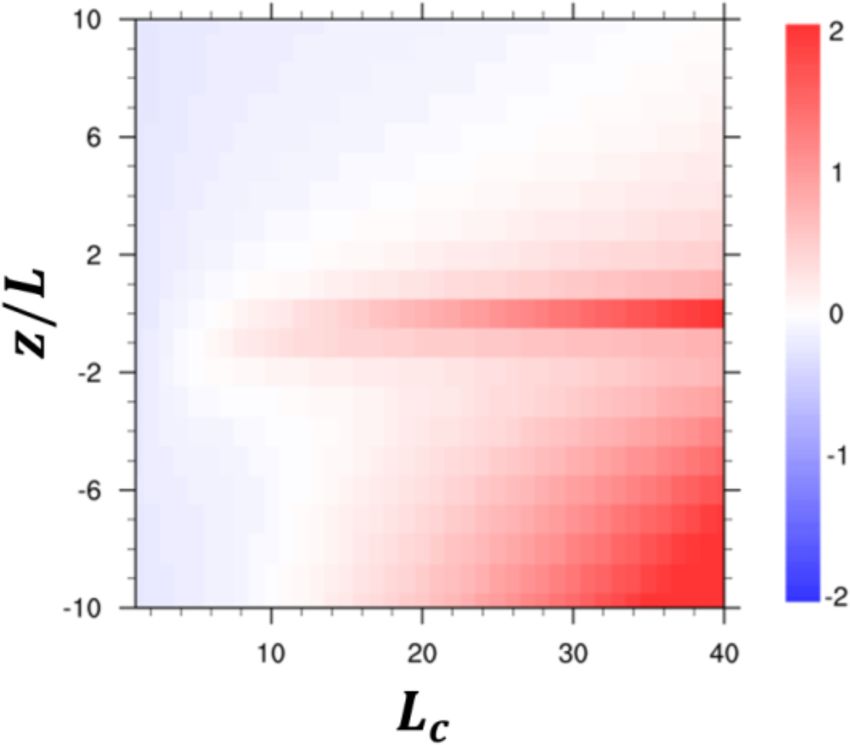
528              J. Lee et al.: Implementation of a roughness sublayer parameterization in the WRF version 3.7.1 model

Figure 7. (a) Roughness length (m), (b) aerodynamic conductance (m s−1 ), (c) sensible heat flux (W m−2 ), (d) latent heat flux (W m−2 ),
and (e) net radiation (W m−2 ) at a given atmospheric stability (z/L). The black lines denote offCTL, while the gray lines denote offRSL.

   During the winter simulation period, precipitation was ob-          Despite the increase in λE, precipitation decreased in several
served over an extensive area in the domain, and snow was              regions (Figs. 11b and 13b). The differences were not signif-
dominant over the northeastern side of the domain (Figs. 12b           icant in the summer season, and the skill scores in the YSL
and 13). The overall total precipitation in the YSL scheme             scheme were similar to the default WRF simulation because
increased, and the skill score indicated a better simulation           our implemented RSL parameterization started to converge
of the total amount of precipitation (Table 2, Fig. 13). The           to the default WRF in a smaller Lc (i.e., larger LAI and/or
pattern correlation of precipitation also increased from 0.972         smaller h) and strong synoptic influences by the summer
to 0.978 in the YSL scheme based on 656 rain gauge sta-                heavy rainy period (Table S1 in the Supplement, Figs. S2–
tions, indicating a better match of the precipitation bands.           S6).

Geosci. Model Dev., 13, 521–536, 2020                                                      www.geosci-model-dev.net/13/521/2020/
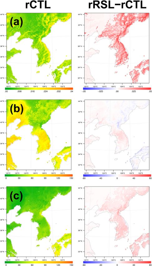
J. Lee et al.: Implementation of a roughness sublayer parameterization in the WRF version 3.7.1 model                             529

Figure 8. (a) Roughness length (m), (b) 10 m wind speed (m s−1 ), and (c) daytime 2 m temperature (K) of the (left) rCTL experiment and
(right) the difference (rRSL–rCTL). The results are averaged over a period of 1 month and masked out over the ocean.

www.geosci-model-dev.net/13/521/2020/                                                      Geosci. Model Dev., 13, 521–536, 2020
530              J. Lee et al.: Implementation of a roughness sublayer parameterization in the WRF version 3.7.1 model

Figure 9. (a) A 1-month mean diurnal variation of 10 m wind speed and (b) the Taylor diagram showing the correlation coefficient, normal-
ized centered root mean square differences (RMSDs), and standard deviations of the models (σm ) normalized by that of observation (σo )
from observation (gray), rCTL experiment (black), and rRSL experiment (red). The vectors indicate the changes of the statistics from rCTL
to rRSL. The arrows indicate those from rCTL to rRSL. Every vector shows the movement toward the observation, thereby suggesting the
model improvement.

Figure 10. Same as in Fig. 9 but for the 2 m temperature.

Table 2. Statistics of the 10 m wind speed, 2 m temperature, and       7   Summary and concluding remarks
rain rate. The top statistics are presented in bold.

                                      rCTL       rRSL                  Turbulent fluxes regulate the planetary boundary layer; thus,
                                                                       they are a crucial process for weather, climate, and air pol-
            10 m wind speed                                            lution simulations. Most of the NWP and climate models are
            Mean bias (m s−1 )           2.4       1.0                 commonly applied for MOST to compute the turbulent fluxes
            RMSE (m s−1 )                3.1       1.8                 near the Earth’s surface. MOST can be only applicable in
                                                                       the inertial layer and turbulence deviates from MOST in the
            2 m temperature                                            roughness sublayer. Importantly, the roughness sublayer, the
            Mean bias (K)             –0.92     −1.16                  important compartment of the SL, has not been properly pa-
            RMSE (K)                   2.74      2.67                  rameterized in the model. Increasing the computing power
            Rain rate
                                                                       enables us to use more vertical layers in the atmospheric
                                                                       models. Accordingly, the RSL must be incorporated into the
            Mean bias (mm h−1 )     −0.018     –0.018                  model properly to simulate the atmospheric processes in the
            RMSE (mm h−1 )           0.194      0.187                  gray zone. This study proposed the YSL scheme, which in-
            Pattern correlation      0.972      0.978                  corporated the RSL into the WRF model, based on the RSL
                                                                       model proposed by Harman and Finnigan (2007, 2008) and
                                                                       Harman (2012). We also investigated the impacts of the RSL

Geosci. Model Dev., 13, 521–536, 2020                                                      www.geosci-model-dev.net/13/521/2020/
J. Lee et al.: Implementation of a roughness sublayer parameterization in the WRF version 3.7.1 model 531 Figure 11. (a) Aerodynamic conductance (m s−1 ), (b) daytime sensible heat flux (W m−2 ), and (c) daytime latent heat flux (W m−2 ) of the (left) rCTL experiment and (right) the difference (rRSL–rCTL). The results are averaged over a period of 1 month and masked out over the ocean. www.geosci-model-dev.net/13/521/2020/ Geosci. Model Dev., 13, 521–536, 2020
532              J. Lee et al.: Implementation of a roughness sublayer parameterization in the WRF version 3.7.1 model

Figure 12. (a) Difference of the soil moisture (m3 m−3 ) (rRSL–rCTL) and (b) snow cover (%) of rCTL. The results are averaged over a
period of 1 month and masked out over the ocean.

Figure 13. (a) The 1-month accumulated precipitation of the rCTL experiment (mm) and (b) difference (rRSL–rCTL). (c) Taylor diagram
showing the correlation coefficient, normalized centered RMSD, and the standard deviations of models (σm ) normalized by that of the
observation (σo ) and from the rain rate (mm h−1 ) of the rCTL experiment (black) and the rRSL experiment (red) during 1 month at 656 rain
gauges.

parameterization on the weather and climate simulations. For           ters had a maximum in the weakly unstable condition and
these purposes, we designed a series of offline simulations            in larger Lc (i.e., large h or small LAI). In most condi-
with an idealized boundary condition and real case simula-             tions, the YSL scheme provided a larger roughness length,
tions to evaluate the performance of the YSL scheme against            thereby producing a wind speed slower than that of the re-
the observation data.                                                  vised MM5 SL scheme. The YSL scheme simulated a colder
   The 1-D offline simulation revealed that the YSL scheme             surface temperature in the unstable conditions.
successfully reproduced the features reported in various                  Meanwhile, the real case simulation showed that the RSL-
canopies. The RSL function, φ̂c , asymptotically increased             incorporated WRF produced a larger z0 than the default
to 1, and the vertical gradients of the wind speed and the tem-        WRF. This increase in z0 and its change with atmospheric
perature decreased in the RSL as z increased, thereby con-             stability eventually made substantial impacts on wind, and
verging to the MOST prediction. Notably, unlike the typical            temperature near the surface, momentum transfer, surface
assignment of the roughness parameters (i.e., z0 , dt , and β)         energy balance, and precipitation. First, an increase of z0
as a constant, the roughness parameters are functions of the           produced larger momentum fluxes and a smaller 10 m wind
atmospheric stability (z/L) and Lc . The roughness parame-             speed when the YSL scheme was applied, leading to the

Geosci. Model Dev., 13, 521–536, 2020                                                      www.geosci-model-dev.net/13/521/2020/
J. Lee et al.: Implementation of a roughness sublayer parameterization in the WRF version 3.7.1 model                        533

mitigation of positive bias in the wind speed in the revised          Our results indicate that the RSL parameterization can be
MM5 SL scheme. The larger z0 also made increases in the            a promising option for resolving the typical overestimation
available energy. This increased available energy is related to    of the surface wind speed of the WRF model, particularly in
the surface cooling caused by the increases in the latent heat     the tall vegetation and low LAI, with slight increase of com-
fluxes in the wet surface conditions when the RSL parame-          puting time (e.g., Hu et al., 2010, 2013; Shimada and Oh-
terization is applied. As a result, these changes in the climate   sawa, 2011; Shimada et al., 2011; Wyszogrodzki et al., 2013;
near the surface and the surface energy balance resulted in        Lee and Hong, 2016). The improvement caused by the RSL
more precipitation, thereby giving a better simulation of the      parameterization is useful in air quality modeling and wind
amount of precipitation and its spatial pattern.                   energy estimation by better weather and climate in the plan-
                                                                   etary boundary layer. A further study is necessary to evaluate
                                                                   the characteristics of the YSL scheme in various cases par-
                                                                   ticularly at gray-zone resolutions.

www.geosci-model-dev.net/13/521/2020/                                                  Geosci. Model Dev., 13, 521–536, 2020
534 J. Lee et al.: Implementation of a roughness sublayer parameterization in the WRF version 3.7.1 model
Appendix A: List of symbols and definitions
Symbols Definitions
a Leaf area density
Bib Bulk Richardson number, at the lowest model layer
cd Drag coefficient at the leaf level
cp Specific heat for air
cs Effective heat transfer coefficient for nonturbulent processes (Carlson and Boland, 1978; Jiménez et al., 2012)
C Variable at z, such as u and T
C0 C at z = z0
Ch C at h
C∗ Scale of C
d0 Conventionally defined zero-plane displacement height
dt Redefined zero-plane displacement height in Harman and Finnigan (2007)
√
f Parameter related the depth scale of the scalar profile (≡ 21 ( 1 + 4rc Sc − 1))
g Gravitational acceleration
ga Aerodynamic conductance
h Canopy height
k von Kármán constant
lm Mixing length for momentum
L Obukhov length
4h
Lc Canopy penetration depth (≡ (cd a)−1 = LAI )
LAI Leaf area index
p Pressure at z
q Water vapor mixing ratio at z
rc Canopy Stanton number
SW Downward shortwave radiation
Sc Turbulent Schmidt number at canopy top
Sm Soil moisture
T Air temperature at z
T2 Air temperature at 2 m
Tsk Skin temperature
u Wind speed at z
u10 Wind speed at 10 m
uh Wind speed at h
u∗ Friction velocity
un−1
∗ Previous time step value of u∗
z Height from d0
z̃ Height from terrain surface
z0 Roughness length
zl Viscous sublayer depth = 0.001 (Carlson and Boland, 1978; Jiménez et al., 2012)
zr Height of the lowest model layer
zr /L Atmospheric stability
β u∗ /uh
βN β at neutral condition (= 0.374)
θa Potential temperature of the air at zr
θva Virtual potential temperature of the air at zr
θvg Virtual potential temperature of the air at ground
ρ Density of air
φC Similarity function of C
φ̂C RSL function of C
ψC Integrated similarity function of C
ψh Integrated similarity function of heat
ψm Integrated similarity function of momentum
ψ̂C Integrated RSL function of C
ψ̂h Integrated RSL function of heat
ψ̂m Integrated RSL function of momentum
Geosci. Model Dev., 13, 521–536, 2020 www.geosci-model-dev.net/13/521/2020/J. Lee et al.: Implementation of a roughness sublayer parameterization in the WRF version 3.7.1 model 535
Code and data availability. The source code of the Weather Re- Bonan, G. B., Patton, E. G., Harman, I. N., Oleson, K. W., Finni-
search and Forecasting model (WRF) (Skamarock et al., 2008) is gan, J. J., Lu, Y., and Burakowski, E. A.: Modeling canopy-
available at http://www2.mmm.ucar.edu/wrf/users/downloads.html induced turbulence in the Earth system: a unified parameteriza-
(last access: 4 February 2020). The source code of the YSL tion of turbulent exchange within plant canopies and the rough-
scheme and the modeling output presented in this study are avail- ness sublayer (CLM-ml v0), Geosci. Model Dev., 11, 1467–
able at Zenodo (https://doi.org/10.5281/zenodo.3555537) (last ac- 1496, https://doi.org/10.5194/gmd-11-1467-2018, 2018.
cess: 4 February 2020). The National Centers for Environmen- Brunet, Y. and Irvine, M. R.: The control of coherent eddies in vege-
tal Prediction Final Analysis data that were used as initial and tation canopies: streamwise structure spacing, canopy shear scale
boundary conditions are available at https://rda.ucar.edu/datasets/ and atmospheric stability, Bound.-Lay. Meteorol., 94, 139–163,
ds083.2 (last access: 4 February 2020) (National Centers for En- 2000.
vironmental Prediction, National Weather Service, NOAA, US De- Carlson, T. N. and Boland, F. E.: Analysis of urban-rural canopy
partment of Commerce, 2000). The observation data used for using a surface heat flux/temperature model, Bound.-Lay. Mete-
the model evaluation can be downloaded at the Korea Meteo- orol., 17, 998–1013, 1978.
rological Administration data portal (https://data.kma.go.kr/data/ de Ridder, K.: Bulk transfer relations for the roughness sublayer,
grnd/selectAsosRltmList.do?pgmNo=36) (last access: 4 Febru- Bound.-Lay. Meteorol., 134, 257–267, 2010.
ary 2010) or are available upon request to the corresponding author Dupont, S. and Patton, E. G.: Momentum and scalar trans-
(jhong@yonsei.ac.kr/http://eapl.yonsei.ac.kr, last access: 10 Febru- port within a vegetation canopy following atmospheric stabil-
ary 2020). ity and seasonal canopy changes: the CHATS experiment, At-
mos. Chem. Phys., 12, 5913–5935, https://doi.org/10.5194/acp-
12-5913-2012, 2012.
Supplement. The supplement related to this article is available on- Finnigan, J. J.: Turbulence in plant canopies, Annu. Rev. Fluid
line at: https://doi.org/10.5194/gmd-13-521-2020-supplement. Mech., 32, 519–571, 2000.
Harman, I. N.: The role of roughness sublayer dynamics within
surface exchange schemes, Bound.-Lay. Meteorol., 142, 1–20,
Author contributions. JL and JH contributed to the code develop- 2012.
ment for the YSL scheme, data analysis, and manuscript prepara- Harman, I. N. and Finnigan, J. J.: A simple unified theory for flow in
tion. YN and PAJ contributed to the writing and editing of the paper the canopy and roughness sublayer, Bound.-Lay. Meteorol., 123,
and data analysis. 339–363, 2007.
Harman, I. N. and Finnigan, J. J.: Scalar concentration profiles in
the canopy and roughness sublayer, Bound.-Lay. Meteorol., 129,
323–351, 2008.
Competing interests. The authors declare that they have no conflict
Hong, J., Kim, J., Miyata, A., and Harazono, Y.: Basic characteris-
of interest.
tics of canopy turbulence in a homogeneous rice paddy, J. Geo-
phys. Res., 107, 4623, https://doi.org/10.1029/2002JD002223,
2002.
Acknowledgements. Our thanks go to the editor and anonymous re- Hong, J.-W., Hong, J., Kwon, E., and Yoon, D.: Temporal dynamics
viewers for their constructive comments. of urban heat island correlated with the socio-economic develop-
ment over the past half-century in Seoul, Korea, Environ. Pollut.,
https://doi.org/10.1016/j.envpol.2019.07.102, in press, 2019.
Financial support. This research has been supported by the Na- Hu, X. M., Nielsen-Gammon, J. W., and Zhang, F.: Evaluation of
tional Research Foundation of Korea grant funded by the South three planetary boundary layer schemes in the WRF model, J.
Korean government (MSIT) (grant no. NRF-2018R1A5A1024958), Appl. Meteorol. Clim., 49, 1831–1844, 2010.
the Korea Meteorological Administration Research and Develop- Hu, X. M., Klein, P. M., and Xue, M.: Evaluation of the updated
ment Program (grant no. KMI2018-03512), and the Korea Polar YSU planetary boundary layer scheme within WRF for wind
Research Institute (grant no. PN20081). resource and air quality assessments, J. Geophys. Res.-Atmos.,
118, 10490–10505, https://doi.org/10.1002/jgrd.50823, 2013.
Jiménez, P. A., Dudhia, J., González-Rouco, J. F., Navarro, J., Mon-
Review statement. This paper was edited by Jatin Kala and re- távez, J. P., and García-Bustamante, E.: A revised scheme for the
viewed by two anonymous referees. WRF surface layer formulation, Mon. Weather Rev., 140, 898–
918, 2012.
Kaimal, J. C. and Finnigan, J. J.: Atmospheric boundary layer flows:
their structure and measurement, Oxford University Press, Ox-
References ford, UK, 1994.
Lee, J. and Hong, J.: Implementation of spaceborne lidar-retrieved
Arnqvist, J. and Bergström, H.: Flux-profile relation with roughness canopy height in the WRF model, J. Geophys. Res., 121, 6863–
sublayer correction, Q. J. Roy. Meteorol. Soc., 141, 1191–1197, 6876, 2016.
2015. Mölder, M., Grelle, A., Lindroth, A., and Halldin, S.: Flux-profile
Basu, S. and Lacser, A.: A Cautionary Note on the Use of Monin– relationships over a boreal forest – roughness sublayer correc-
Obukhov Similarity Theory in Very High-Resolution Large- tions, Agr. Forest Meteorol., 98, 645–658, 1999.
Eddy Simulations, Bound.-Lay. Meteorol., 163, 351–355, 2017.
www.geosci-model-dev.net/13/521/2020/ Geosci. Model Dev., 13, 521–536, 2020536 J. Lee et al.: Implementation of a roughness sublayer parameterization in the WRF version 3.7.1 model Monin, A. S. and Obukhov, A. M. F.: Basic laws of turbulent mixing Shimada, S. and Ohsawa, T.: Accuracy and characteristics of off- in the surface layer of the atmosphere, Contrib. Geophys. Slovak shore wind speeds simulated by WRF, Scient. Online Lett. At- Acad. Sci., 151, 163–187, 1954. mos., 7, 21–24, 2011. Obukhov, A. M.: Turbulence in an atmosphere with a nonuniform Shimada, S., Ohsawa, T., Chikaoka, S., and Kozai, K.: Accuracy of temperature, Trudy Inst. Theor. Geofiz. AN SSSR 1, 95–115, the wind speed profile in the lower PBL as simulated by the WRF 1946. model, Scient. Online Lett. Atmos., 7, 109–112, 2011. Physick, W. L. and Garratt, J. R.: Incorporation of a high-roughness Shin, H. H., Hong, S. Y., and Dudhia, J.: Impacts of the low- lower boundary into a mesoscale model for studies of dry depo- est model level height on the performance of planetary bound- sition over complex terrain, Bound.-Lay. Meteorol., 74, 55–71, ary layer parameterizations, Mon. Weather Rev., 140, 664–682, 1995. 2012. Raupach, M.: Drag and drag partition on rough surfaces, Bound.- Skamarock, W. C., Klemp, J. B., Dudhia, J., Gill, D. O., Barker, D. Lay. Meteorol., 60, 375–395, 1992. M., Wang, W., and Powers, J. G.: A description of the Advanced Raupach, M., Finnigan, J. J., and Brunet, Y.: Coherent eddies Research WRF version 3, Tech. Rep. Note NCAR/TN-4751STR, and turbulence in vegetation canopies: the mixing-layer analogy, National Center for Atmospheric Research, Boulder, CO, USA, Springer, Netherlands, 1996. 113 pp., https://doi.org/10.5065/D68S4MVH, 2008. Sellers, P. J., Mintz, Y. C. S. Y., Sud, Y. E. A., and Dalcher, A.: A Taylor, K. E.: Summarizing multiple aspects of model performance simple biosphere model (SiB) for use within general circulation in a single diagram, J. Geophys. Res., 106, 7183–7192, 2001. models, J. Atmos. Sci., 43, 505–531, 1986. Wenzel, A., Kalthoff, N., and Horlacher, V.: On the profiles of wind Sellers, P. J., Randall, D. A., Collatz, G. J., Berry, J. A., Field, C. velocity in the roughness sublayer above a coniferous forest, B., Dazlich, D. A., Zhang, C., Collelo, G. D., and Bounoua, L.: Bound.-Lay. Meteorol., 84, 219–230, 1997. A revised land surface parameterization (SiB2 ) for atmospheric Wyszogrodzki, A. A., Liu, Y., Jacobs, N., Childs, P., Zhang, Y., GCMs. Part I: Model formulation, J. Climate, 9, 676–705, 1996. Roux, G., and Warner, T. T.: Analysis of the surface tempera- Shapkalijevski, M. M., Moene, A. F., Ouwersloot, H. G., Patton, ture and wind forecast errors of the NCAR-AirDat operational E. G., and Vilà-Guerau de Arellano, J.: Influence of Canopy CONUS 4-km WRF forecasting system, Meteorol. Atmos. Phys., Seasonal Changes on Turbulence Parameterization within the 122, 125–143, 2013. Roughness Sublayer over an Orchard Canopy, J. Appl. Meteo- Zahumenský, I.: Guidelines on quality control procedures for data rol. Clim., 55, 1391–1407, 2016. from automatic weather stations, World Meteorological Organi- Shapkalijevski, M. M., Ouwersloot, H. G., Moene, A. F., and zation, Switzerland, 2004. de Arrellano, J. V.-G.: Integrating canopy and large-scale ef- Zahn, E., Dias, N. L., Araújo, A., Sá, L. D. A., Sörgel, M., fects in the convective boundary-layer dynamics during the Trebs, I., Wolff, S., and Manzi, A.: Scalar turbulent behavior in CHATS experiment, Atmos. Chem. Phys., 17, 1623–1640, the roughness sublayer of an Amazonian forest, Atmos. Chem. https://doi.org/10.5194/acp-17-1623-2017, 2017. Phys., 16, 11349–11366, https://doi.org/10.5194/acp-16-11349- Shaw, R. H., Den Hartog, G., and Neumann, H. H.: Influence of fo- 2016, 2016. liar density and thermal stability on profiles of Reynolds stress and turbulence intensity in a deciduous forest, Bound.-Lay. Me- teorol., 45, 391–409, 1988. Geosci. Model Dev., 13, 521–536, 2020 www.geosci-model-dev.net/13/521/2020/
You can also read