Learning models for visual 3D localization with implicit mapping
←
→
Page content transcription
If your browser does not render page correctly, please read the page content below
Learning models for visual 3D localization
                                                             with implicit mapping

                                               Dan Rosenbaum, Frederic Besse, Fabio Viola, Danilo J. Rezende, S. M. Ali Eslami
                                                                         DeepMind, London, UK
                                                     {danro,fbesse,fviola,danilor,aeslami}@google.com
arXiv:1807.03149v2 [cs.CV] 12 Dec 2018

                                                                                       Abstract

                                                  We consider learning based methods for visual localization that do not require
                                                  the construction of explicit maps in the form of point clouds or voxels. The
                                                  goal is to learn an implicit representation of the environment at a higher, more
                                                  abstract level. We propose to use a generative approach based on Generative
                                                  Query Networks (GQNs, [8]), asking the following questions: 1) Can GQN capture
                                                  more complex scenes than those it was originally demonstrated on? 2) Can GQN
                                                  be used for localization in those scenes? To study this approach we consider
                                                  procedurally generated Minecraft worlds, for which we can generate images of
                                                  complex 3D scenes along with camera pose coordinates. We first show that
                                                  GQNs, enhanced with a novel attention mechanism can capture the structure of 3D
                                                  scenes in Minecraft, as evidenced by their samples. We then apply the models to
                                                  the localization problem, comparing the results to a discriminative baseline, and
                                                  comparing the ways each approach captures the task uncertainty.

                                         1   Introduction

                                         The problem of identifying the position of the camera that captured an image of a scene has been
                                         studied extensively for decades [34, 33, 4]. With applications in domains such as robotics and
                                         autonomous driving, a considerable amount of engineering effort has been dedicated to developing
                                         systems for different versions of the problem. One formulation, often referred to as simply ‘localiza-
                                         tion’, assumes that a map of the 3D scene is provided in advance and the goal is to localize any new
                                         image of the scene relative to this map. A second formulation, commonly referred to as ‘Simultaneous
                                         Localization and Mapping’ (SLAM), assumes that there is no prespecified map of the scene, and
                                         that it should be estimated concurrently with the locations of each observed image. Research on
                                         this topic has focused on different aspects and challenges including: estimating the displacement
                                         between frames in small time scales, correcting accumulated drifts in large time scales (also known
                                         as ‘loop closure’), extracting and tracking features from the observed images (e.g. [17, 20]), reducing
                                         computational costs of inference (graph-based SLAM [9]) and more.
                                         Although this field has seen huge progress, performance is still limited by several factors [4].
                                         One key limitation stems from reliance on hand-engineered representations of various components
                                         of the problem (e.g. key-point descriptors as representations of images and occupancy grids as
                                         representations of the map), and it has been argued that moving towards systems that operate using
                                         more abstract representations is likely to be beneficial [25, 18]. Considering the map, it is typically
                                         specified as either part of the input provided to the system (in localization) or part of its expected
                                         output (in SLAM). This forces algorithm designers to define its structure explicitly in advance, e.g.
                                         either as 3D positions of key-points, or an occupancy grid of a pre-specified resolution. It is not
                                         always clear what the optimal representation is, and the need to pre-define this structure is restricting
                                         and can lead to sub-optimal performance.

                                         Third workshop on Bayesian Deep Learning (NeurIPS 2018), Montréal, Canada.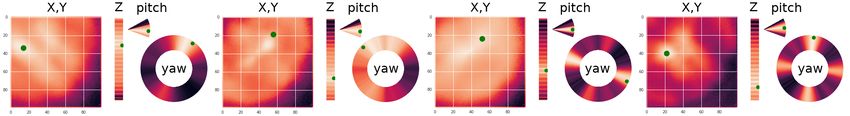
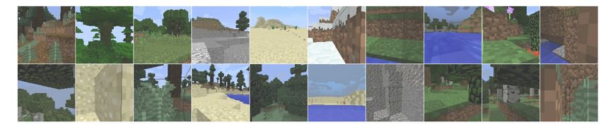
Figure 1: The Minecraft random walk dataset for localization in 3D scenes. We generate random
trajectories in the Minecraft environment, and collect images along the trajectory labelled by camera
pose coordinates (x,y,z yaw and pitch). Bottom: Images from random scenes. Top: The localization
problem setting - for a new trajectory in a new scene, given a set of images and corresponding camera
poses (the ‘context’), predict the camera pose of an additional observed image (the ‘target’, in green).

 In this work, we investigate the problem of localization with implicit mapping, by considering the
‘re-localization’ task, using learned models with no explicit form of map. Given a collection of
‘context’ images with known camera poses, ‘re-localization’ is defined as finding the relative camera
 pose of a new image which we call the ‘target’. This task can also be viewed as loop closure without
 an explicit map. We consider deep models that learn implicit representations of the map, where at
 the price of making the map less interpretable, the models can capture abstract descriptions of the
 environment and exploit abstract cues for the localization problem.
In recent years, several methods for localization that are based on machine learning have been
proposed. Those methods include models that are trained for navigation tasks that require localiza-
tion. In some cases the models do not deal with the localization explicitly, and show that implicit
localization and mapping can emerge using learning approaches [19, 7, 2, 39]. In other cases, the
models are equipped with specially designed spatial memories, that can be thought of as explicit
maps [42, 10, 22]. Other types of methods tackle the localization problem more directly using
models that are either trained to output the relative pose between two images [40, 36], or models like
PoseNet [14], trained for re-localization, where the model outputs the camera pose of a new image,
given a context of images with known poses. Models like PoseNet do not have an explicit map, and
therefore have an opportunity to learn more abstract mapping cues that can lead to better performance.
However, while machine learning approaches outperform hand-crafted methods in many computer
vision tasks, they are still far behind in visual localization. A recent study [38] shows that a method
based on traditional structure-from-motion approaches [26] significantly outperforms PoseNet. One
potential reason for this, is that most machine learning methods for localization, like PoseNet, are
discriminative, i.e. they are trained to directly output the camera pose. In contrast, hand-crafted
methods are usually constructed in a generative approach, where the model encodes geometrical
assumptions in the causal direction, concerning the reconstruction of the images given the poses of
the camera and some key-points. Since localization relies heavily on reasoning with uncertainty,
modeling the data in the generative direction could be key in capturing the true uncertainty in the
task. Therefore, we investigate here the use of a generative learning approach, where on one hand
the data is modeled in the same direction as hand-crafted methods, and on the other hand there is no
explicit map structure, and the model can learn implicit and abstract representations.
A recent generative model that has shown promise in learning representations for 3D scene structure is
the Generative Query Network (GQN) [8]. The GQN is conditioned on different views of a 3D scene,
and trained to generate images from new views of the same scene. Although the model demonstrates
generalization of the representation and rendering capabilities to held-out 3D scenes, the experiments
are in simple environments that only exhibit relatively well-defined, small-scale structure, e.g. a few
objects in a room, or small mazes with a few rooms. In this paper, we ask two questions: 1) Can the
GQN scale to more complex, visually rich environments? 2) Can the model be used for localization?
To this end, we propose a dataset of random walks in the game Minecraft (figure 1), using the Malmo
platform [13]. We show that coupled with a novel attention mechanism, the GQN can capture the 3D
structure of complex Minecraft scenes, and can use this for accurate localization. In order to analyze

                                                   2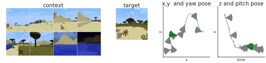
the advantages and shortcomings of the model, we compare to a discriminative version of it, similar
to previously proposed methods.
In summary, our contributions are the following: 1) We suggest a generative approach to localization
with implicit mapping and propose a dataset for it. 2) We enhance the GQN using a novel sequential
attention model, showing it can capture the complexity of 3D scenes in Minecraft. 3) We show that
GQN can be used for localization, finding that it performs comparably to our discriminative baseline
when used for point estimates, and investigate how the uncertainty is captured in each approach.

2   Data for localization with implicit mapping
In order to study machine learning approaches to visual localization with implicit mapping, we
create a dataset of random walks in a visually rich simulated environment. We use the Minecraft
environment through the open source Malmo platform [13]. Minecraft is a popular computer game
where a player can wander in a virtual world, and the Malmo platform allows us to connect to the
game engine, control the player and record data. Since the environment is procedurally generated,
we can generate sequences of images in an unlimited number of different scenes. Figure 1 shows
the visual richness of the environment and the diversity of the scene types including forests, lakes,
deserts, mountains etc. The images are not realistic but nevertheless contain many details such as
trees, leaves, grass, clouds, and also different lighting conditions.
Our dataset consists of 6000 sequences of 100 images each generated by a blind exploration policy
based on simple heuristics (see appendix A for details). We record images at a resolution of 128 × 128
although for all the experiments in this paper we downscale to 32 × 32. Each image is recorded along
with a 5 dimensional vector of camera pose coordinates consisting of the x, y, z position and yaw and
pitch angles (omitting the roll as it is constant). Figure 1 also demonstrates the localization task: For
every sequence we are given a context of images along with their camera poses, and an additional
target image with unknown pose. The task is to find the camera pose of the target image.
While other datasets for localization with more realistic images have been recently proposed [1, 29,
5, 30], we choose to use Minecraft data for several reasons. First, in terms of the visual complexity,
it is a smaller step to take from the original GQN data, which still poses interesting questions on
the model’s ability to scale. The generative approach is known to be hard to scale but nevertheless
has advantages and this intermediate dataset allows us to demonstrate them. The second reason, is
that Minecraft consists of outdoors scenes which compared to indoor environments, contain a 3D
structure that is larger in scale, and where localization should rely on more diverse clues such as
using both distant key-points (e.g. mountains in the horizon) and closer structure (e.g. trees and
bushes). Indoor datasets also tend to be oriented towards sequential navigation tasks relying much on
strong priors of motion. Although in practice, agents moving in an environment usually have access
to dense observations, and can exploit the fact that the motion between subsequent observations is
very small, we focus here on localization with a sparse observation set, since we are interested in
testing the model’s ability to capture the underlying structure of the scene only from observations and
without any prior on the camera’s motion. One example for this setting is when multiple agents can
broadcast observations to help each other localize. In this case there are usually constraints on the
network bandwidth and therefore on the number of observations, and there is also no strong prior on
the camera poses which all come from different cameras.

3   Model
The localization problem can be cast as an inference task in the probabilistic graphical model
presented in figure 2a. Given an unobserved environment E (which can also be thought of as the
map), any observed image X depends on the environment E and on the pose P of the camera that
captured the image P r(X|P, E). The camera pose P depends on the environment and perhaps some
prior, e.g. a noisy odometry sensor. In this framing, localization is an inference task involving the
posterior probability of the camera pose which can be computed using Bayes’ rule:
                                               1
                              P r(P |X, E) = P r(X|P, E)P r(P |E)                                 (1)
                                               Z
In our case, the environment is only implicitly observed through the context, a set of image and
camera pose pairs, which we denote by C = {xi , pi }. We can use the context to estimate the

                                                   3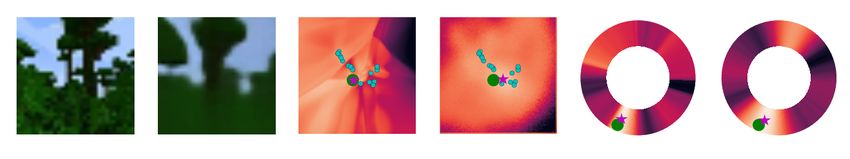
context          representation network             generation network
       camera-pose         environment
                                         camera                                        target
   prior     P                     E     pose image                                    camera pose

                                         camera
                                         pose image                     +                                 predicted
                                                                               r
                       X                                                +                                 image
                                                                                        1    2       L
                                         camera                           scene
                           observed
      generative                         pose image                   representation
                           image
      discriminative

(a) Localization as inference                                     (b) The GQN model
Figure 2: Localization as probabilistic inference (a). The observed images X depend on the environ-
ment E and the camera pose P . To predict P r(P |X), in the generative approach, we use a model of
P r(X|P ) (green) and apply Bayes’ rule. In the discriminative approach we directly train a model
of P r(P |X) (red). In both cases the environment is implicitly modeled given a context of (image,
camera pose) pairs C = {xi , pi }. In the GQN model (b), the context is processed by a representation
network and the resulting scene representation is fed to a recurrent generation network with L layers,
predicting an image given a camera pose.

environment Ê(C) and use the estimate for inference:
                                              1
                           P r(P |X, C) = P r(X|P, Ê(C))P r(P |Ê(C))                                  (2)
                                             Z
Relying on the context to estimate the environment E can be seen as an empirical Bayes approach,
where the prior for the data is estimated (in a point-wise manner) at test time from a set of observations.
In order to model the empirical Bayes likelihood function P r(X|P, Ê(C)) we consider the Generative
Query Network (GQN) model [8] (figure 2b). We use the same model as described in the GQN paper,
which has two components: a representation network, and a generation network. The representation
network processes each context image along with its corresponding camera pose coordinates using a
6-layer convolutional neural network. The camera pose coordinates are combined to each image by
concatenating a 7 dimensional vector of x, y, z, sin(yaw), cos(yaw), sin(pitch), cos(pitch) to the
features of the neural network in the middle layer. The output of the network for each image is then
added up resulting in a single scene representation. Conditioned on this scene representation and
the camera pose of a new target view, the generation network which consists of a conditional latent-
variable model DRAW [8] with 8 recurrent layers, generates a probability distribution of the target
image P rGQN (X|P, C). We use this to model P r(X|P, Ê(C)), where the scene representation r
serves as the point-wise estimate of the environment Ê(C).
Given a pre-trained GQN model as a likelihood function, and a prior over the camera pose P r(P |C),
localization can be done by maximizing the posterior probability of equation 2 (MAP inference):
                       arg max P r(P |X, C) = arg max log P rGQN (X|P, C) + log P (P |C)                          (3)
                               P                      P
With no prior, we can simply resort to maximum likelihood, omitting the second term above. The
optimization problem can be a hard problem in itself, and although we show some results for simple
cases, this is usually the main limitation of this generative approach.

3.1    Attention

One limitation of the GQN model is the fact that the representation network compresses all the
information from the context images and poses to a single global representation vector r. Although
the GQN has shown the ability to capture the 3D structure of scenes and generate samples of new
views that are almost indistinguishable from ground truth, it has done so in fairly simple scenes
with only a few objects in each scene and limited variability. In more complex scenes with much
more visual variability, it is unlikely for a simple representation network with a fixed size scene
representation to be able to retain all the important information of the scene. Following previous
work on using attention for making conditional predictions [37, 23, 21], we propose a variation of the
GQN model that relies on attention rather than a parametric representation of the scene.
We enhance the GQN model using an attention mechanism on patches inspired by [23] (figure 3),
where instead of passing the context images through a representation network, we extract from each

                                                           4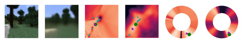
context    extract all                      generation network
 camera        image          target                                             for layer 1 to L:
 pose image    patches        camera pose                                         key = f(state)
 camera                                                              predicted
                                                                                  scores = key ·
 pose image                  attention                               image        weights
                                                                                       P = softmax(scores)
                                            1    2      L                         v=      weights ·
 camera                                                                           state = g(state, v)
 pose image

                         patch dictionary
                     (a) A GQN model with attention.                                (b) Attention computation

Figure 3: (a) Instead of conditioning on a parametric representation of the scene, all patches from
context images are stored in a dictionary, and each layer of the generation network can access them
through an attention mechanism. In each layer, the key is computed as a function of the generation
network’s recurrent state, and the result v is fed back to the layer (b).

of the images all the 8 by 8 patches and concatenate to each the camera poses and the 2D coordinates
of the patch within the image. For each patch we also compute a key using a convolutional neural
network, and place all patches and their corresponding keys in a large dictionary, which is passed
to the generation network. In the generation network, which is based on the DRAW model with 8
recurrent layers, a key is computed at every layer from the current state, and used to perform soft
attention on the patch dictionary. The attention is performed using a dot-product with all the patches’
keys, normalizing the results to one using a softmax, and using them as the weights in a weighted
sum of all patches. The resulting vector is then used by the generation network in the same way as the
global representation vector is used in the parametric GQN model. See appendix B for more details.
In this sequential attention mechanism, the key in each layer depends on the result of the attention at
the previous layer, which allows the model to use a more sophisticated attention strategy, depending
both on the initial query and on patches and coordinates that previous layers attended to.

3.2   A discriminative approach

As a baseline for the proposed generative approach based on GQN, we use a discriminative model
which we base on a ‘reversed-GQN’. This makes the baseline similar to previously proposed methods
(see section 4), but also similar to the proposed GQN model in terms of architecture and the
information it has access to, allowing us to make more informative comparisons.
While the generative approach is to learn models in the P → X direction and invert them using
Bayes’ rule as described above, a discriminative approach would be to directly learn models in the
X → P direction. In order to model P r(P |X, C) directly, we construct a ‘reversed-GQN’ model,
by using the same GQN model described above, but ‘reversing’ the generation network, i.e. using
a model that is conditioned on the target image, and outputs a distribution over the camera pose.
The output of the model is a set of categorical distributions over the camera pose space, allowing
multi-modal distributions to be captured. In order to keep the output dimension manageable, we
split the camera pose coordinate space to four components: 1) the x, y positions, 2) the z position,
3) the yaw angle, and 4) the pitch angle. To implement this we process the target image using a
convolutional neural network, where the scene representation is concatenated to the middle layer, and
compute each probability map using an MLP.
We also implement an attention based version of this model, where the decoder’s MLP is preceded by
a sequential attention mechanism with 10 layers, comparable to the attention in the generative model.
For more details on all models see appendix B.
Although the discriminative approach is a more direct way to solve the problem and will typically
result in much faster inference at test time, the generative approach has some aspects that can prove
advantageous: it learns a model in the causal direction, which might be easier to capture, easier to
interpret and easier to break into modular components; and it learns a more general problem not
specific to any particular task and free from any prior on the solution, such as the statistics that
generated the trajectories. In this way it can be used for tasks which it was not trained for, for example
different types of trajectories, or for predicting the x,y location in a different spatial resolution.

                                                        5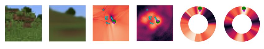
generative loss             pixel MSE             discriminative loss           pose MSE

Figure 4: The loss and predictive MSE for both the generative direction and the discriminative
direction. The attention model results in lower loss and lower MSE in both directions.

4   Related work
In recent years, machine learning has been increasingly used in localization and SLAM methods. In
one type of methods, a model is trained to perform some navigation task that requires localization,
and constructed using some specially designed spatial memory that encourages the model to encode
the camera location explicitly [42, 22, 10, 11, 12, 28, 21]. The spatial memory can then be used to
extract the location. Other models are directly trained to estimate either relative pose between image
pairs [40, 36], or camera re-localization in a given scene [14, 38, 6].
All these methods are discriminative, i.e. they are trained to estimate the location (or a task that
requires a location estimate) in an end-to-end fashion, essentially modeling P r(P |X) in the graphical
model of figure 2. In that sense, our baseline model using a reversed-GQN, is similiar to the learned
camera re-localization methods like PoseNet [14], and in fact can be thought of as an adaptive (or
meta-learned) PoseNet, where the model is not trained on one specific scene, but rather inferred at
test time, thus adapting to different scenes. The reason we implement an adaptive PoseNet rather
than comparing to the original version is that in our setting it is unlikely for PoseNet to successfully
learn the network’s weights from scratch for every scene, which contains only a small number of
images. In addition, having a baseline which is as close as possible to the proposed model makes the
direct comparison of the approaches easier.
In contrast to the more standard discriminative approach, the model that we propose using GQN, is a
generative approach that captures P r(X|P ), making it closer to traditional hand-crafted localization
methods that are usually constructed with geometric rules in the generative direction. For example,
typical methods based on structure-from-motion (SfM) [16, 41, 31, 26] optimize a loss involving
reconstruction in image space given pose estimates (the same way GQN is trained).
The question of explicit vs. implicit mapping in hand-crafted localization methods, has been studied
in [27], where it was shown that re-localization relying on image matching can outperform methods
that need to build complete 3D models of a scene. With learned models, the hope is that we can get
even more benefit from implicit mapping since it allows the model to learn abstract mapping cues that
are hard to define in advance. Two recent papers, [3, 32], take a somewhat similar approach to ours
by encoding depth information into an implicit encoding, and training the models based on image
reprojection error. Other recent related work [43, 35] take a generative approach to pose estimation
but explicitly model depth maps or 3D shapes.

5   Training results
We train the models on the Minecraft random walk data, where each sample consists of 20 context
images and 1 target image, from a random scene. The images are drawn randomly from the sequence
(containing 100 images) in order to reduce the effect of the prior on the target camera pose due to
the sequential nature of the captured images. The loss we optimize in the generative direction is the
negative variational lower bound on the log-likelihood over the target image, since the GQN contains
a DRAW model with latent variables. For the discriminative direction with the reversed GQN which
is fully deterministic, we minimize the negative log-likelihood over the target camera pose.
Figure 4 shows the training curves for the generative and discriminative directions. In both cases we
compare between the standard parametric model and the attention model. We also compare the MSE
of the trained models, computed in the generative direction by the L2 distance between the predicted

                                                   6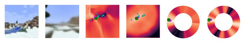
ground
truth

samples

camera pose
probability
maps

Figure 5: Generated samples from the generative model (middle), and the whole output distribution
for the discriminative model (bottom). Both were computed using the attention models, and each
image and pose map is from a different scene conditioned on 20 context images. The samples capture
much of the structure of the scenes including the shape of mountains, the location of lakes, the
presence of large trees etc. The distribution of camera pose computed with the reversed GQN shows
the model’s uncertainty, and the distribution’s mode is usually close to the ground truth (green dot).

image and the ground-truth image, and in the discriminative direction by the L2 distance between
the most likely camera pose and the ground truth one. All results are computed on a held out test
set containing scenes that were not used in training, and are similar to results on the training set. A
notable result is that the attention models improve the performance significantly. This is true for both
the loss and the predictive MSE, and for both the discriminative and generative directions.
Figure 5 shows generated image samples from the generative model, and the predicted distribution
over the camera pose space from the reversed GQN model. All results are from attention based
models, and each image and camera pose map comes from a different scene from a held out test
set, conditioned on 20 context images. Image samples are blurrier than the ground truth but they
capture the underlying structure of the scene, including the shape of mountains, the location of lakes,
the presence of big trees etc. For the reversed GQN model, the predicted distribution shows the
uncertainty of the model, however the mode of the distribution is usually close to the ground truth
camera pose. The results show that some aspects of the camera pose are easier than others. Namely,
predicting the height z and the pitch angle are much easier than the x, y location and yaw angle. At
least for the pitch angle this can be explained by the fact that it can be estimated from the target
image alone, not relying on the context. As for the yaw angle, we see a frequent pattern of high
probability areas around multiples of 90 degrees. This is due to the cubic nature of the Minecraft
graphics, allowing the estimate of the yaw angle up to any 90 degrees rotation given the target image
only. This last phenomena is a typical one when comparing discriminative methods to generative
ones, where the former is capable of exploiting shortcuts in the data.
One interesting feature of models with attention, is that they can be analyzed by observing where they
are attending, shedding light on some aspects of the way they work. Figure 6 shows the attention in
three different scenes. Each row shows 1) the target image, 2) the x,y trajectory containing the poses
of all context images (in black) and the pose of the target image (in green), and 3) the context images
with a red overlay showing the patches with high attention weights. In each row we show the context
images twice, once with the attention weights of the generative model, and once with the attention
weights of the discriminative model. In both cases we show the total attention weights summed over
all recurrent layers. A first point to note is that the attention weights are sparse, focusing on a small
number of patches in a small number of images. The attention focuses on patches with high contrast
like the edges between the sky and the ground. In these aspects, the model has learned to behave
similarly to the typical components of hand crafted localization methods - detecting informative
feature points (e.g. Harris corner detection), and constructing a sparse computation graph by pruning
out the irrelevant images (e.g. graph-SLAM). A second point to note is the difference between the
generative and discriminative attention, where the first concentrates on fewer images, covering more
space within them, and the second is distributed between more images. Since the generative model is
queried using a camera pose, and the discriminative model using an image, it is perhaps not surprising
that the resulting attention strategies tend to be position-based and appearance-based respectively.
For more examples see the video available at https://youtu.be/iHEXX5wXbCI.

                                                   7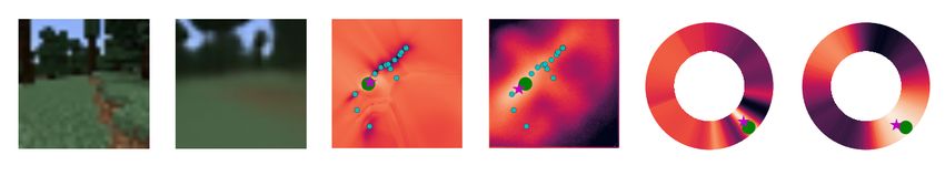
target      x,y
                                generative attention                   discriminative attention
    image    trajectory

Figure 6: Attention over the context images in the generative and discriminative directions. The
total attention weights are shown as a red overlay, using the same context images for both directions.
Similar to hand-crafted feature point extraction and graph-SLAM, the learned attention is sparse and
prunes out irrelevant images. While the generative attention is mainly position based, focusing on
one or two of the nearest context images, the discriminative attention is based more on appearance,
searching all context images for patches resembling the target. See also supplementary video.

6     Localization

We compare the generative and discriminative models ability to perform localization, i.e. find the
camera pose of a target image, given a context of image and camera pose pairs. For the discriminative
models we simply run a forward pass and get the probability map of the target’s camera pose. For the
generative model, we fix the target image and optimize the likelihood by searching over the camera
pose used to query the model. We do this for both the x,y position, and the yaw, using grid search
with the same grid values as the probability maps that are predicted by the discriminative model. The
optimization of the x,y values, and the yaw values is done separately while fixing all other dimensions
of the camera pose to the ground truth values. We do this without using a prior on the camera pose,
essentially implementing maximum likelihood inference rather than MAP.
Figure 7 shows the results for a few held-out scenes comparing the output of the discriminative
model, with the probability map computed with the generative model. For both directions we use
the best trained models which are the ones with attention. We see that in most cases the maximum
likelihood estimate (magenta star) is a good predictor of the ground truth value (green circle) for both
models. However it is interesting to see the difference in the probability maps of the generative and
discriminative directions. One aspect of this difference is that while in the discriminative direction
the x,y values near the context points tend to have high probability, for the generative model it is the
opposite. This can be explained by the fact that the discriminative model captures the posterior of
the camera pose, which also includes the prior, consisting of the assumption that the target image
was taken near context images. The generative model only captures the likelihood P r(X|P ), and
therefore is free from this prior, resulting in an opposite effect where the area near context images
tend to have very low probability and a new image is more likely to be taken from an unexplored
location. See appendix figure 9 for more examples.
Table 1 shows a quantitative comparison of models with and without attention, with varying number
of context points. The first table compares the MSE of the maximum likelihood estimate of the x,y
position and the yaw angle, by computing the square distance from the ground truth values. The table
shows the improvement due to attention, and that as expected, more context images result in better
estimates. We also see that the generative models estimates have a lower MSE for all context sizes.
This is true even though the generative model does not capture the prior on camera poses and can
therefore make very big mistakes by estimating the target pose far from the context poses. The second
table compares the log probability of the ground truth location for the x,y position and yaw angles
(by using the value in the probability map cell which is closest to the ground truth). Here we see that
the discriminative model results in higher probability. This can be caused again by the fact that the
generative model does not capture the prior of the data and therefore distributes a lot of probability

                                                   8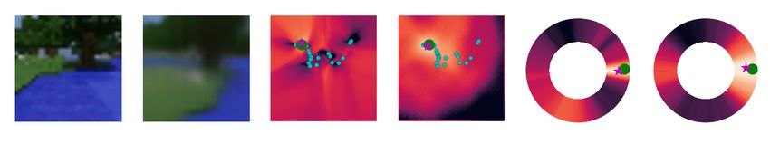
Table 1: Localization with a varying number of context images. Using attention (‘+att’) and more
context images leads to better results. Even with no prior on poses, the generative+attention model
results in better MSE. However the discriminative+attention model assigns higher probability to the
ground-truth pose since the prior allows it to concentrate more mass near context poses.
                      x,y position         yaw angle                                  x,y position            yaw angle

                                                               log-probability
       context      5      10     20     5    10     20                             5      10      20      5     10     20
 MSE

         disc     0.27 0.25 0.27       0.25 0.21 0.17                             -8.14 -7.24 -7.08      -3.27 -3.08 -3.02
         gen      0.41 0.36 0.35       0.16 0.14 0.15                            -10.19 -9.08 -8.55      -5.95 -5.16 -4.74
       disc+att   0.17 0.12 0.09       0.21 0.15 0.11                             -7.65 -6.47 -5.74      -3.56 -3.29 -3.08
       gen+att    0.11 0.08 0.07       0.06 0.06 0.05                             -7.56 -6.62 -6.00      -4.48 -4.06 -3.66

                           sample at          x,y                   x,y                        yaw              yaw
        target image     target position   generative         discriminative                generative     discriminative

Figure 7: Localization with the generative and discriminative models - target image, a sample drawn
using the ground-truth pose, and probability maps for x,y position and yaw angle (bright=high prob.).
The generative maps are computed by querying the model with all possible pose coordinates, and the
discriminative maps are simply the model’s output. The poses of the context images are shown in
cyan, target image in green and maximum likelihood estimates in magenta. The generative maps are
free from the prior on poses in the training data giving higher probability to unexplored areas.

mass across all of the grid. We validate this claim by computing the log probability in the vicinity of
all context poses (summing the probability of a 3 by 3 grid around each context point) and indeed
get a log probability of -4.1 for the generative direction compared to -1.9 for the discriminative one
(using attention and 20 context images). Another support for the claim that the discriminative model
relies more on the prior of poses rather than the context images is that in both tables, the difference
due to attention is bigger for the generative model compared to the discriminative model.

7      Discussion
We have proposed a formulation of the localization problem that does not involve an explicit map,
where we can learn models with implicit mapping in order to capture higher level abstractions. We
have enhanced the GQN model with a novel attention mechanism, and showed its ability to capture
the underlying structure of complex 3D scenes demonstrated by generating samples of new views
of the scene. We showed that GQN-like models can be used for localization in a generative and
discriminative approach, and described the advantages and disadvantages of each.
When comparing the approaches for localization we have seen that the generative model is better
in capturing the underlying uncertainty of the problem and is free from the prior on the pose that
is induced by the training data. However, its clear disadvantage is that it requires performing
optimization at test time, while the discriminative model can be used by running one forward pass.
We believe that future research should focus on combining the approaches which can be done in
many different ways, e.g. using the discriminative model as a proposal distribution for importance
sampling, or accelerating the optimization using amortized inference by training an inference model
on top of the generative model [24]. While learning based methods, as presented here and in prior
work, have shown the ability to preform localization, they still fall far behind hand-crafted methods
in most cases. We believe that further development of generative methods, which bear some of
the advantages of hand-crafted methods, could prove key in bridging this gap, and coupled with an
increasing availability of real data could lead to better methods also for real-world applications.

                                                          9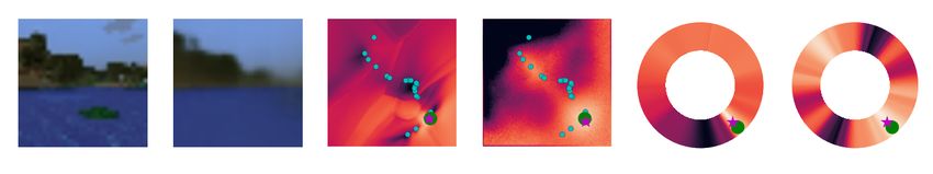
Acknowledgements
We would like to thank Jacob Bruce, Marta Garnelo, Piotr Mirowski, Shakir Mohamed, Scott Reed,
Murray Shanahan and Theophane Weber for providing feedback on the research and the manuscript.

References
 [1] I. Armeni, O. Sener, A. R. Zamir, H. Jiang, I. Brilakis, M. Fischer, and S. Savarese. 3d semantic parsing
     of large-scale indoor spaces. In Proceedings of the IEEE Conference on Computer Vision and Pattern
     Recognition, pages 1534–1543, 2016.

 [2] A. Banino, C. Barry, B. Uria, C. Blundell, T. Lillicrap, P. Mirowski, A. Pritzel, M. J. Chadwick, T. Degris,
     et al. Vector-based navigation using grid-like representations in artificial agents. Nature, page 1, 2018.

 [3] M. Bloesch, J. Czarnowski, R. Clark, S. Leutenegger, and A. J. Davison. Codeslam-learning a compact,
     optimisable representation for dense visual slam. arXiv preprint arXiv:1804.00874, 2018.

 [4] C. Cadena, L. Carlone, H. Carrillo, Y. Latif, D. Scaramuzza, J. Neira, I. Reid, and J. J. Leonard. Past,
     present, and future of simultaneous localization and mapping: Toward the robust-perception age. IEEE
     Transactions on Robotics, 32(6):1309–1332, 2016.

 [5] A. Chang, A. Dai, T. Funkhouser, M. Halber, M. Nießner, M. Savva, S. Song, A. Zeng, and Y. Zhang.
     Matterport3d: Learning from rgb-d data in indoor environments. arXiv preprint arXiv:1709.06158, 2017.

 [6] R. Clark, S. Wang, A. Markham, N. Trigoni, and H. Wen. Vidloc: 6-dof video-clip relocalization. arxiv
     preprint. arXiv preprint arXiv:1702.06521, 2017.

 [7] C. J. Cueva and X.-X. Wei. Emergence of grid-like representations by training recurrent neural networks
     to perform spatial localization. arXiv preprint arXiv:1803.07770, 2018.

 [8] S. A. Eslami, D. J. Rezende, F. Besse, F. Viola, A. S. Morcos, M. Garnelo, A. Ruderman, A. A. Rusu,
     I. Danihelka, et al. Neural scene representation and rendering. Science, 360(6394):1204–1210, 2018.

 [9] G. Grisetti, R. Kummerle, C. Stachniss, and W. Burgard. A tutorial on graph-based slam. IEEE Intelligent
     Transportation Systems Magazine, 2(4):31–43, 2010.

[10] S. Gupta, J. Davidson, S. Levine, R. Sukthankar, and J. Malik. Cognitive mapping and planning for visual
     navigation. arXiv preprint arXiv:1702.03920, 3, 2017.

[11] S. Gupta, D. Fouhey, S. Levine, and J. Malik. Unifying map and landmark based representations for visual
     navigation. arXiv preprint arXiv:1712.08125, 2017.

[12] J. F. Henriques and A. Vedaldi. Mapnet: An allocentric spatial memory for mapping environments. In
     IEEE Conference on Computer Vision and Pattern Recognition, pages 8476–8484, 2018.

[13] M. Johnson, K. Hofmann, T. Hutton, and D. Bignell. The malmo platform for artificial intelligence
     experimentation. 2016.

[14] A. Kendall, M. Grimes, and R. Cipolla. Posenet: A convolutional network for real-time 6-dof camera
     relocalization. In IEEE International Conference on Computer Vision (ICCV), pages 2938–2946, 2015.

[15] D. P. Kingma and J. Ba. Adam: A method for stochastic optimization. arXiv:1412.6980, 2014.

[16] Y. Li, N. Snavely, D. Huttenlocher, and P. Fua. Worldwide pose estimation using 3d point clouds. In
     European conference on computer vision, pages 15–29. Springer, 2012.

[17] D. G. Lowe. Distinctive image features from scale-invariant keypoints. International journal of computer
     vision, 60(2):91–110, 2004.

[18] J. McCormac, A. Handa, A. Davison, and S. Leutenegger. Semanticfusion: Dense 3d semantic mapping
     with convolutional neural networks. In Robotics and Automation (ICRA), 2017 IEEE International
     Conference on, pages 4628–4635. IEEE, 2017.

[19] P. Mirowski, R. Pascanu, F. Viola, H. Soyer, A. J. Ballard, A. Banino, M. Denil, R. Goroshin, L. Sifre, et al.
     Learning to navigate in complex environments. arXiv preprint arXiv:1611.03673, 2016.

[20] R. Mur-Artal, J. M. M. Montiel, and J. D. Tardos. Orb-slam: a versatile and accurate monocular slam
     system. IEEE Transactions on Robotics, 31(5):1147–1163, 2015.

                                                       10
[21] E. Parisotto, D. S. Chaplot, J. Zhang, and R. Salakhutdinov. Global pose estimation with an attention-based
recurrent network. arXiv preprint arXiv:1802.06857, 2018.
[22] E. Parisotto and R. Salakhutdinov. Neural map: Structured memory for deep reinforcement learning. arXiv
preprint arXiv:1702.08360, 2017.
[23] S. Reed, Y. Chen, T. Paine, A. v. d. Oord, S. Eslami, D. J. Rezende, O. Vinyals, and N. de Freitas. Few-shot
autoregressive density estimation: Towards learning to learn distributions. 2017.
[24] D. Rosenbaum and Y. Weiss. The return of the gating network: combining generative models and
discriminative training in natural image priors. In Advances in Neural Information Processing Systems,
pages 2683–2691, 2015.
[25] R. F. Salas-Moreno, R. A. Newcombe, H. Strasdat, P. H. Kelly, and A. J. Davison. Slam++: Simultaneous
localisation and mapping at the level of objects. In Computer Vision and Pattern Recognition (CVPR),
2013 IEEE Conference on, pages 1352–1359. IEEE, 2013.
[26] T. Sattler, B. Leibe, and L. Kobbelt. Efficient & effective prioritized matching for large-scale image-based
localization. IEEE Transactions on Pattern Analysis & Machine Intelligence, (9):1744–1756, 2017.
[27] T. Sattler, A. Torii, J. Sivic, M. Pollefeys, H. Taira, M. Okutomi, and T. Pajdla. Are large-scale 3d models
really necessary for accurate visual localization? In 2017 IEEE Conference on Computer Vision and
Pattern Recognition (CVPR), pages 6175–6184. IEEE, 2017.
[28] N. Savinov, A. Dosovitskiy, and V. Koltun. Semi-parametric topological memory for navigation. arXiv
preprint arXiv:1803.00653, 2018.
[29] M. Savva, A. X. Chang, A. Dosovitskiy, T. Funkhouser, and V. Koltun. Minos: Multimodal indoor
simulator for navigation in complex environments. arXiv preprint arXiv:1712.03931, 2017.
[30] S. Song, F. Yu, A. Zeng, A. X. Chang, M. Savva, and T. Funkhouser. Semantic scene completion from
a single depth image. In Computer Vision and Pattern Recognition (CVPR), 2017 IEEE Conference on,
pages 190–198. IEEE, 2017.
[31] L. Svärm, O. Enqvist, F. Kahl, and M. Oskarsson. City-scale localization for cameras with known vertical
direction. IEEE transactions on pattern analysis and machine intelligence, 39(7):1455–1461, 2017.
[32] C. Tang and P. Tan. Ba-net: Dense bundle adjustment network. arXiv preprint arXiv:1806.04807, 2018.
[33] S. Thrun, W. Burgard, and D. Fox. Probabilistic robotics. MIT press, 2005.
[34] B. Triggs, P. F. McLauchlan, R. I. Hartley, and A. W. Fitzgibbon. Bundle adjustment—a modern synthesis.
In International workshop on vision algorithms, pages 298–372. Springer, 1999.
[35] S. Tulsiani, A. A. Efros, and J. Malik. Multi-view consistency as supervisory signal for learning shape and
pose prediction. arXiv preprint arXiv:1801.03910, 2018.
[36] B. Ummenhofer, H. Zhou, J. Uhrig, N. Mayer, E. Ilg, A. Dosovitskiy, and T. Brox. Demon: Depth and
motion network for learning monocular stereo. In IEEE Conference on computer vision and pattern
recognition (CVPR), volume 5, page 6, 2017.
[37] O. Vinyals, C. Blundell, T. Lillicrap, D. Wierstra, et al. Matching networks for one shot learning. In
Advances in Neural Information Processing Systems, pages 3630–3638, 2016.
[38] F. Walch, C. Hazirbas, L. Leal-Taixe, T. Sattler, S. Hilsenbeck, and D. Cremers. Image-based localization
using lstms for structured feature correlation. In Int. Conf. Comput. Vis.(ICCV), pages 627–637, 2017.
[39] G. Wayne, C.-C. Hung, D. Amos, M. Mirza, A. Ahuja, A. Grabska-Barwinska, J. Rae, P. Mirowski,
J. Z. Leibo, A. Santoro, et al. Unsupervised predictive memory in a goal-directed agent. arXiv preprint
arXiv:1803.10760, 2018.
[40] A. R. Zamir, T. Wekel, P. Agrawal, C. Wei, J. Malik, and S. Savarese. Generic 3d representation via pose
estimation and matching. In European Conference on Computer Vision, pages 535–553. Springer, 2016.
[41] B. Zeisl, T. Sattler, and M. Pollefeys. Camera pose voting for large-scale image-based localization. In
Proceedings of the IEEE International Conference on Computer Vision, pages 2704–2712, 2015.
[42] J. Zhang, L. Tai, J. Boedecker, W. Burgard, and M. Liu. Neural slam. arXiv preprint arXiv:1706.09520,
2017.
[43] T. Zhou, M. Brown, N. Snavely, and D. G. Lowe. Unsupervised learning of depth and ego-motion from
video. In CVPR, volume 2, page 7, 2017.
11A The Minecraft random walk dataset for localization
To generate the data we use the Malmo platform [13], an open source project allowing access to the
Minecraft engine. Our dataset consists of 6000 sequences of random walks consisting of 100 images
each. We use 1000 sequences as a held-out test set. The sequences are generated using a simple
heuristic-based blind policy as follows:
We generate a new world and a random initial position, and wait for the agent to drop to the ground.
For 100 steps:
1. Make a small random rotation and walk forward.
2. With some small probability make a bigger rotation.
3. If no motion is detected jump and walk forward, or make a bigger rotation
4. Record image and camera pose.
We prune out sequences where there was no large displacement or where all images look the same
(e.g. when starting in the middle of the ocean, or when quickly getting stuck in a hole), however in
some cases our exploration policy results in close up images of walls, or even underwater images
which might make the localization challenging.
We use 5 dimensional camera poses consisting of x, y, z position and yaw and pitch angles (omitting
the roll as it is constant). We record images in a resolution of 128 × 128 although for all the
experiments in this paper we downscale to 32 × 32. We normalize the x,y,z position such that most
scenes contain values between -1 and 1.
B Model details
The basic model that we use is the Generative Query Network (GQN) as described in [8]. In the
representation network, every context image is processed by a 6 layer convolutional neural network
(CNN) outputting a representation with spatial dimension of 8 × 8 and 64 channels. We add the
camera pose information of each image after 3 layers of the CNN by broadcasting the values of
x, y, z, sin(yaw), cos(yaw), sin(pitch), cos(pitch) to the whole spatial dimension and concatenate
as additional 7 channels. The output of each image is added up to a single scene representation
of 8 × 8 × 64. The architecture of the CNN we use is: [k=2,s=2,c=32] → [k=3,s=1,c=32] →
[k=2,s=2,c=64] → [k=3,s=1,c=32] → [k=3,s=1,c=32] → [k=3,s=1,c=64], where for each layer ‘k’
stands for the kernel size, ‘s’ for the stride, and ‘c’ for the number of output channels.
In the generation network we use the recurrent DRAW model as described in [8] with 8 recurrent
layers and representation dimension of 8 × 8 × 128 (used as both the recurrent state and canvas
dimensions). The model is conditioned on both the scene representation and the camera pose query
by injecting them (using addition) to the biases of the LSTM’s in every layer. The output of the
generation network is a normal distribution with a fixed standard deviation of 0.3.
In order to train the model, we optimize the negative variational lower bound on the log-likelihood,
using Adam [15] with a batch size of 36, where each example comes from a random scene in
Minecraft, and contains 20 context images and 1 target image. We train the model for 4M iterations,
and anneal the output standard deviation starting from 1.5 in the first iteration, down to 0.3 in the
300K’th iteration, keeping it constant in further iterations.
B.1 Reversed GQN
The reversed GQN model we use as a discriminative model is based on the GQN described above.
We use the same representation network, and a new decoder that we call the localization network,
which is queried using the target image, and outputs a distribution of camera poses (see figure 8). In
order to make the output space manageable, we divide it to 4 log-probability maps:
1. A matrix over x, y values between -1 and 1, quantized in a 0.02 resolution.
2. A vector over z values between -1 and 1, quantized in a 0.02 resolution.
3. A vector over yaw values between -180 and 180 degrees, quantized in a 1 degree resolution.
12context representation network localization network
camera target
pose image image
camera
pose image + predicted
r
+ camera pose
camera scene
pose image representation
Figure 8: The reversed GQN model. A similar architecture to GQN, where the generation network
is ‘reversed’ to form a localization network, which is queried using a target image, and predicts its
camera pose.
4. A vector over pitch values between -20 and 30 degrees, quantized in a 1 degree resolution.
The localization network first processes the image query using a CNN with the following specifica-
tions: [k=3,s=2,c=32] → [k=3,s=2,c=64] → [k=3,s=1,c=64] → [k=1,s=1,c=64] → [k=1,s=1,c=64],
resulting in an intermediate representation of 8 × 8 × 64. Then it concatenates the scene represen-
tation computed by the representation network and processes the result using another CNN with:
[k=3,s=1,c=64] → [k=3,s=1,c=64] → [k=3,s=1,c=64] → [k=5,s=1,c=4]. Each of the 4 channels of
the last layer is used to generate one of the 4 log-probability maps using an MLP with 3 layers, and a
log-softmax normalizer. Figure 5 in the main paper shows examples of the resulting maps.
B.2 Attention GQN
In the attention GQN model, instead of a scene encoder as described above, all 8 × 8 × 3 patches are
extracted from the context images with an overlap of 4 pixels and placed in a patch dictionary, along
with the camera pose coordinates, the 2D patch coordinates within the image (the x,y, position in
image space), and a corresponding key. The keys are computed by running a CNN on each image
resulting in a 8 × 8 × 64 feature map, and extracting the (channel-wise) vector corresponding to
each pixel. The architecture of the CNN is [k=2,s=2,c=32] → [k=3,s=1,c=32] → [k=2,s=2,c=64]
→ [k=1,s=1,c=32] → [k=1,s=1,c=32] → [k=1,s=1,c=64], such that every pixel in the output feature
map corresponds to a 4 × 4 shift in the original image. The keys are also concatenated to the patches.
Given the patch dictionary, we use an attention mechanism within the recurrent layers of the generation
network based on DRAW as follows. In each layer we use the recurrent state to compute a key
using a CNN of [k=1,s=1,c=64] → [k=1,s=1,c=64] followed by spatial average pooling. The key is
used to query the dictionary by computing the dot product with all dictionary keys, normalizing the
results using a softmax. The normalized dot products, are used as weights in a weighted sum over
all dictionary patches and keys (using the keys as additional values). See pseudo-code in figure 3b.
The result is injected to the computation of each layer in the same way as the scene representation
is injected in the standard GQN. Since the state in each layer of the recurrent DRAW depends on
the computation of the previous layer, the attention becomes sequential, with multiple attention keys
where each key depends on the result of the attention with the previous key.
In order to implement attention in the discriminative model, and make it comparable to the sequential
attention in DRAW, we implement a similar recurrent network used only for the attention. This is
done by adding 10 recurrent layers between layer 5 and 6 of the localization network’s CNN. Like in
DRAW, a key is computed using a 2 layer CNN of [k=1,s=1,c=64] → [k=1,s=1,c=64] followed by
spatial average pooling. The key is used for attention in the same way as in DRAW, and the result
is processed through a 3 layer MLP with 64 channels and concatenated to the recurrent state. This
allows the discriminative model to also use a sequential attention strategy where keys depend on the
attention in previous layers.
13sample at x,y x,y yaw yaw
target image target position generative discriminative generative discriminative
Figure 9: Localization with the generative and discriminative models - target image, a sample drawn
using the ground-truth pose, and probability maps for the x,y position and yaw angles. The generative
maps are computed by querying the model with all possible pose coordinates, and the discriminative
maps are simply the model’s output. The poses of the context images are shown in cyan, target image
in green and maximum likelihood estimates in magenta. The generative maps are free from the prior
in the training data (that target poses are close to the context poses) giving higher probability to
unexplored areas and lower probabilities to areas with context images which are dissimilar to the
target.
14You can also read