Cross-Iteration Batch Normalization
←
→
Page content transcription
If your browser does not render page correctly, please read the page content below
Cross-Iteration Batch Normalization

                                                 Zhuliang Yao1, 2 *             Yue Cao2       Shuxin Zheng2       Gao Huang1                                Stephen Lin2
                                                                            1                         2
                                                                              Tsinghua University       Microsoft Research Asia
                                             {yzl17@mails.,gaohuang@}tsinghua.edu.cn                              {yuecao,Shuxin.Zheng,stevelin}@microsoft.com
arXiv:2002.05712v3 [cs.LG] 25 Mar 2021

                                                                     Abstract                                            In BN, it is assumed that the distribution statistics for the
                                                                                                                      examples within each mini-batch reflect the statistics over
                                             A well-known issue of Batch Normalization is its signifi-                the full training set. While this assumption is generally valid
                                         cantly reduced effectiveness in the case of small mini-batch                 for large batch sizes, it breaks down in the small batch size
                                         sizes. When a mini-batch contains few examples, the statis-                  regime [18, 31, 9], where noisy statistics computed from
                                         tics upon which the normalization is defined cannot be re-                   small sets of examples can lead to a dramatic drop in per-
                                         liably estimated from it during a training iteration. To ad-                 formance. This problem hinders the application of BN to
                                         dress this problem, we present Cross-Iteration Batch Nor-                    memory-consuming tasks such as object detection [20, 3],
                                         malization (CBN), in which examples from multiple recent                     semantic segmentation [15, 2] and action recognition [30],
                                         iterations are jointly utilized to enhance estimation qual-                  where batch sizes are limited due to memory constraints.
                                         ity. A challenge of computing statistics over multiple itera-                   Towards improving estimation of statistics in the small
                                         tions is that the network activations from different iterations              batch size regime, alternative normalizers have been pro-
                                         are not comparable to each other due to changes in net-                      posed. Several of them, including Layer Normalization
                                         work weights. We thus compensate for the network weight                      (LN) [1], Instance Normalization (IN) [28], and Group Nor-
                                         changes via a proposed technique based on Taylor polyno-                     malization (GN) [31], compute the mean and variance over
                                         mials, so that the statistics can be accurately estimated and                the channel dimension, independent of batch size. Differ-
                                         batch normalization can be effectively applied. On object                    ent channel-wise normalization techniques, however, tend
                                         detection and image classification with small mini-batch                     to be suitable for different tasks, depending on the set of
                                         sizes, CBN is found to outperform the original batch nor-                    channels involved. Although GN is designed for detec-
                                         malization and a direct calculation of statistics over pre-                  tion task, the slow inference speed limits its practical usage.
                                         vious iterations without the proposed compensation tech-                     On the other hand, synchronized BN (SyncBN) [18] yields
                                         nique. Code is available at https://github.com/                              consistent improvements by processing larger batch sizes
                                         Howal/Cross-iterationBatchNorm.                                              across multiple GPUs. These gains in performance come at
                                                                                                                      the cost of additional overhead needed for synchronization
                                                                                                                      across the devices.
                                         1. Introduction                                                                  A seldom explored direction for estimating better statis-
                                                                                                                      tics is to compute them over the examples from multiple re-
                                             Batch Normalization (BN) [10] has played a significant
                                                                                                                      cent training iterations, instead of from only the current iter-
                                         role in the success of deep neural networks. It was intro-
                                                                                                                      ation as done in previous techniques. This can substantially
                                         duced to address the issue of internal covariate shift, where
                                                                                                                      enlarge the pool of data from which the mean and variance
                                         the distribution of network activations changes during train-
                                                                                                                      are obtained. However, there exists an obvious drawback
                                         ing iterations due to the updates of network parameters.
                                                                                                                      to this approach, in that the activation values from differ-
                                         This shift is commonly believed to be disruptive to network
                                                                                                                      ent iterations are not comparable to each other due to the
                                         training, and BN alleviates this problem through normaliza-
                                                                                                                      changes in network weights. As shown in Figure 1, directly
                                         tion of the network activations by their mean and variance,
                                                                                                                      calculating the statistics over multiple iterations, which we
                                         computed over the examples within the mini-batch at each
                                                                                                                      refer to as Naive CBN, results in lower accuracy.
                                         iteration. With this normalization, network training can be
                                         performed at much higher learning rates and with less sen-                      In this paper, we present a method that compensates for
                                         sitivity to weight initialization.                                           the network weight changes among iterations, so that ex-
                                                                                                                      amples from preceding iterations can be effectively used to
                                            * This work is done when Zhuliang Yao is an intern at Microsoft Re-       improve batch normalization. Our method, called Cross-
                                         search Asia. Correspondence to: Yue Cao (yuecao@microsoft.com).              Iteration Batch Normalization (CBN), is motivated by the

                                                                                                                  1
window size (k) of CBN cause of its simplicity and effectiveness [26, 11].
1 1 2 4 8 16
After the introduction of Batch Normalization [10], the
70 normalization of activations has become nearly as preva-
lent. By normalizing hidden activations by their statis-
Top-1 accuracy
69
tics within each mini-batch, BN effectively alleviates the
68 vanishing gradient problem and significantly speeds up the
BN training of deep networks. To mitigate the mini-batch size
67 BRN
GN
dependency of BN, a number of variants have been pro-
66 Naive CBN posed, including Layer Normalization (LN) [1], Instance
CBN (ours) Normalization (IN) [28], Group Normalization (GN) [31],
65
32 16 8 4 2 1 and Batch Instance Normalization (BIN) [17]. The motiva-
batch size per iter tion of LN is to explore more suitable statistics for sequen-
Figure 1. Top-1 classification accuracy vs. batch sizes per it- tial models, while IN performs normalization in a manner
eration. The base model is a ResNet-18 [6] trained on Ima- similar to BN but with statistics only for each instance. GN
geNet [21]. The accuracy of BN [10] drops rapidly when the batch achieves a balance between IN and LN, by dividing features
size is reduced. BRN [9] stabilizes BN a little but still has trou- into multiple groups along the channel dimension and com-
ble with smaller batch sizes. GN [31] exhibits stable performance puting the mean and variance within each group for nor-
but underperforms BN on adequate batch sizes. CBN compen- malization. BIN introduces a learnable method for auto-
sates for the reduced batch size per GPU by exploiting approxi- matically switching between normalizing and maintaining
mated statistics from recent iterations (Temporal window size de-
style information, enjoying the advantages of both BN and
notes how many recent iterationss are utilized for statistics com-
putation). CBN shows relatively stable performance over different
IN on style transfer tasks. Cross-GPU Batch Normaliza-
batch sizes. Naive CBN, which directly calculates statistics from tion (CGBN or SyncBN) [18] extends BN across multiple
recent iterations without compensation, is shown not to work well. GPUs for the purpose of increasing the effective batch size.
Though providing higher accuracy, it introduces synchro-
nization overhead to the training process. Kalman Normal-
observation that network weights change gradually, in- ization (KN) [29] presents a Kalman filtering procedure for
stead of abruptly, between consecutive training iterations, estimating the statistics for a network layer from the layer’s
thanks to the iterative nature of Stochastic Gradient De- observed statistics and the computed statistics of previous
scent (SGD). As a result, the mean and variance of exam- layers.
ples from recent iterations can be well approximated for the Batch Renormalization (BRN) [9] is the first attempt to
current network weights via a low-order Taylor polynomial, utilize the statistics of recent iterations for normalization. It
defined on gradients of the statistics with respect to the net- does not compensate for the statistics from recent iterations,
work weights. The compensated means and variances from but rather it down-weights the importance of statistics from
multiple recent iterations are averaged with those of the cur- distant iterations. This down-weighting heuristic, however,
rent iteration to produce better estimates of the statistics. does not make the resulting statistics “correct”, as the statis-
In the small batch size regime, CBN leads to appreciable tics from recent iterations are not of the current network
performance improvements over the original BN, as exhib- weights. BRN can be deemed as a special version of our
ited in Figure 1. The superiority of our proposed approach Naive CBN baseline (without Taylor polynomial approxi-
is further demonstrated through more extensive experiments mation), where distant iterations are down-weighted.
on ImageNet classification and object detection on COCO.
Recent work have also investigated the normalization of
These gains are obtained with negligible overhead, as the
network parameters. In Weight Normalization (WN) [22],
statistics from previous iterations have already been com-
the optimization of network weights is improved through a
puted and Taylor polynomials are simple to evaluate. With
reparameterization of weight vectors into their length and
this work, it is shown that cues for batch normalization can
direction. Weight Standardization (WS) [19] instead repa-
successfully be extracted along the time dimension, open-
rameterizes weights based on their first and second mo-
ing a new direction for investigation.
ments for the purpose of smoothing the loss landscape of the
optimization problem. To combine the advantages of mul-
2. Related Work tiple normalization techniques, Switchable Normalization
The importance of normalization in training neural net- (SN) [16] and Sparse Switchable Normalization (SSN) [24]
works has been recognized for decades [11]. In general, make use of differentiable learning to switch among differ-
normalization can be performed on three components: input ent normalization methods.
data, hidden activations, and network parameters. Among The proposed CBN takes an activation normalization ap-
them, input data normalization is used most commonly be- proach that aims to mitigate the mini-batch dependency of
2BN. Different from existing techniques, it provides a way to µt−τ (θt−τ ) and νt−τ (θt−τ ) of the (t − τ )-th iteration are
effectively aggregate statistics across multiple training iter- computed under the network weights θt−τ , making them
ations. obsolete for the current iteration. As a consequence, di-
rectly aggregating statistics from multiple iterations pro-
3. Method duces inaccurate estimates of the mean and variance, lead-
ing to significantly worse performance.
3.1. Revisiting Batch Normalization We observe that the network weights change smoothly
The original batch normalization (BN) [10] whitens the between consecutive iterations, due to the nature of
activations of each layer by the statistics computed within a gradient-based training. This allows us to approxi-
mini-batch. Denote θt and xt,i (θt ) as the network weights mate µt−τ (θt ) and νt−τ (θt ) from the readily available
and the feature response of a certain layer for the i-th exam- µt−τ (θt−τ ) and νt−τ (θt−τ ) via a Taylor polynomial, i.e.,
ple in the t-th mini-batch. With these values, BN conducts
the following normalization: ∂µt−τ (θt−τ )
µt−τ (θt ) =µt−τ (θt−τ ) + (θt − θt−τ )
∂θt−τ (5)
xt,i (θt ) − µt (θt ) + O(||θt − θt−τ ||2 ),
x̂t,i (θt ) = p , (1)
σt (θt )2 +
∂νt−τ (θt−τ )
where x̂t,i (θt ) is the whitened activation with zero mean νt−τ (θt ) =νt−τ (θt−τ ) + (θt − θt−τ )
∂θt−τ (6)
and unit variance, is a small constant added for numerical
+ O(||θt − θt−τ ||2 ),
stability, and µt (θt ) and σt (θt ) are the mean and variance
computed for all the examples from the current mini-batch, where ∂µt−τ (θt−τ )/∂θt−τ and ∂νt−τ (θt−τ )/∂θt−τ are
i.e., gradients of the statistics with respect to the network
m
1 X weights, and O(||θt − θt−τ ||2 ) denotes higher-order terms
µt (θt ) = xt,i (θt ), (2) of the Taylor polynomial, which can be omitted since the
m i=1
v first-order term dominates when (θt − θt−τ ) is small.
u
u1 X m In Eq. (5) and Eq. (6), the gradients ∂µt−τ (θt−τ )/∂θt−τ
σt (θt ) = t (xt,i (θt ) − µt (θt ))2 and ∂νt−τ (θt−τ )/∂θt−τ cannot be precisely determined
m i=1 (3) at a negligible cost because the statistics µlt−τ (θt−τ ) and
l
p νt−τ (θt−τ ) for a node at the l-th network layer depend
= νt (θt ) − µt (θt )2 ,
on all the network weights prior to the l-th layer, i.e.,
Pm
where νt (θt ) = m 1 2
i=1 xt,i (θt ) , and m denotes the num-
r
∂µlt−τ (θt−τ )/∂θt−τ 6= 0 and ∂νt−τl
(θt−τ )/∂θt−τr
6= 0 for
r
ber of examples in the current mini-batch. The whitened r ≤ l, where θt−τ denotes the network weights at the r-th
activation x̂t,i (θt ) further undergoes a linear transform with layer. Only when r = l can these gradients be derived in
learnable weights, to increase its expressive power: closed form efficiently.
Empirically, we find that as the layer index r decreases
yt,i (θt ) = γ x̂t,i (θt ) + β, (4) ∂µl (θ ) ∂ν l (θ )
(r ≤ l), the partial gradients θt r t and θt r t rapidly di-
t t
where γ and β are the learnable parameters (initialized to minish. These reduced effects of network weight changes
γ = 1 and β = 0 in this work). at earlier layers on the activation distributions in later layers
When the batch size m is small, the statistics µt (θt ) and may perhaps be explained by the reduced internal covari-
σt (θt ) become noisy estimates of the training set statistics, ate shift of BN. Motivated by this phenomenon, which is
thus degrading the effects of batch normalization. In the studied in Appendix C, we propose to truncate these partial
ImageNet classification task for which the BN module was gradients at layer l.
Thus, we further approximate Eq. (5) and Eq. (6) by
originally designed, a batch size of 32 is typical. However,
for other tasks requiring larger models and/or higher im- ∂µlt−τ (θt−τ ) l
age resolution, such as object detection, semantic segmen- µlt−τ (θt ) ≈ µlt−τ (θt−τ ) + l
l
(θt − θt−τ ), (7)
∂θt−τ
tation and video recognition, the typical batch size may be l
l l ∂νt−τ (θt−τ ) l l
as small as 1 or 2 due to GPU memory limitations. The orig- νt−τ (θt ) ≈ νt−τ (θt−τ ) + l
(θt − θt−τ ). (8)
∂θt−τ
inal BN becomes considerably less effective in such cases.
A naive implementation of ∂µlt−τ (θt−τ )/∂θt−τ l
and
3.2. Leveraging Statistics from Previous Iterations l l
∂νt−τ (θt−τ )/∂θt−τ involves computational overhead of
To address the issue of BN with small mini-batches, a O(Cout × Cout × Cin × K), where Cout and Cin denote
naive approach is to compute the mean and variance over the output and input channel dimension of the l-th layer, re-
l
the current and previous iterations. However, the statistics spectively, and K denotes the kernel size of θt−τ . Here,
3Iteration t-2 Iteration t-1 Iteration t
BN
Normalize, Normalize, Normalize,
Affine transform Affine transform Affine transform
mean, variance mean, variance mean, variance
( μt−2 , δt−2 ) ( μt−1 , δt−1 ) ( μt , δt )
Compensated Compensated Compensated
mean, variance mean, variance mean, variance
( μ̄t−2 , δ̄t−2 ) ( μ̄t−1 , δ̄t−1 ) ( μ̄t , δ̄t )
Normalize, Normalize, Normalize,
Affine transform Affine transform Affine transform
CBN
Figure 2. Illustration of BN and the proposed Cross-Iteration Batch Normalization (CBN).
we find that the operation can be implemented efficiently in gradients are backpropagated to the network weights and
O(Cout × Cin × K), thanks to the averaging over feature activations at the current iteration, i.e., θtl and xlt,i (θt ).
responses of µ and ν. See Appendix B for the details. Those of the previous iterations are fixed and do not receive
gradients. Hence, the computation cost of CBN in back-
3.3. Cross-Iteration Batch Normalization propagation is the same as that of BN.
After compensating for network weight changes, we ag- Replacing the BN modules in a network by CBN leads
gregate the statistics of the k − 1 most recent iterations with to only minor increases in computational overhead and
those of the current iteration t to obtain the statistics used in memory footprint. For computation, the additional over-
CBN: head mainly comes from computing the partial derivatives
l l
∂µt−τ (θt−τ )/∂θt−τ and ∂νt−τ (θt−τ )/∂θt−τ , which is
k−1
1X l insignificant in relation to the overhead of the whole
µ̄lt,k (θt ) = µ (θt ), (9)
k τ =0 t−τ network. For memory, the module requires access to the
statistics ({µlt−τ (θt−τ )}k−1 τ =1 and {νt−τ l
(θt−τ )}k−1
τ =1 )
k−1 k−1
l 1X l l
and the gradients ({∂µt−τ (θt−τ )/∂θt−τ }τ =1 and
(θt ), µlt−τ (θt )2 ,
ν̄t,k (θt ) = max νt−τ (10)
k τ =0 {∂νt−τ (θt−τ )/∂θt−τl
}k−1
τ =1 ) computed for the most re-
cent k − 1 iterations, which is also minor compared to
q the rest of the memory consumed in processing the input
l l (θ ) − µ̄l (θ )2 , examples. The additional computation and memory of
σ̄t,k (θt ) = ν̄t,k t t,k t (11)
CBN is reported for our experiments in Table 8.
where µlt−τ (θt ) and νt−τ l
(θt ) are computed from Eq. (7) A key hyper-parameter in the proposed CBN is the tem-
and Eq. (8). In Eq. (10), ν̄t,k l
(θt ) is determined from the poral window size, k, of recent iterations used for statistics
maximum of νt−τ (θt ) and µt−τ (θt )2 in each iteration be-
l l estimation. A broader window enlarges the set of exam-
cause νt−τl
(θt ) ≥ µlt−τ (θt )2 should hold for valid statistics ples, but the example quality becomes increasingly lower
but may be violated by Taylor polynomial approximations for more distant iterations, since the differences in network
in Eq. (7) and Eq. (8). Finally, µ̄lt,k (θt ) and σ̄t,k l
(θt ) are parameters θt and θt−τ become more significant and are
applied to normalize the corresponding feature responses compensated less well using a low-order Taylor polyno-
{xlt,i (θt )}m mial. Empirically, we found that CBN is effective with
i=1 at the current iteration:
a window size up to k = 8 in a variety of settings and
xlt,i (θt ) − µ̄lt,k (θt ) tasks. The only trick is that the window size should be
x̂lt,i (θt ) = q . (12) kept small at the beginning of training, when the network
l (θ )2 +
σ̄t,k t weights change quickly. Thus, we introduce a burn-in pe-
riod of length Tburn-in for the window size, where k = 1 and
With CBN, the effective number of examples used to CBN degenerates to the original BN. In our experiments,
compute the statistics for the current iteration is k times the burn-in period is set to 25 epochs on ImageNet image
as large as that for the original BN. In training, the loss classification and 3 epochs on COCO object detection by
4batch size per iter #examples for statistics Norm axis
IN #bs/GPU * #GPU 1 (spatial)
LN #bs/GPU * #GPU 1 (channel, spatial)
GN #bs/GPU * #GPU 1 (channel group, spatial)
BN #bs/GPU * #GPU #bs/GPU (batch, spatial)
syncBN #bs/GPU * #GPU #bs/GPU * #GPU (batch, spatial, GPU)
CBN #bs/GPU * #GPU #bs/GPU * temporal window (batch, spatial, iteration)
Table 1. Comparison of different feature normalization methods. #bs/GPU denotes batch size per GPU.
default. IN LN GN CBN BN
Table 1 compares CBN with other feature normalization Top-1 acc 64.4±0.2 67.9±0.2 68.9±0.1 70.2±0.1 70.2±0.1
methods. The key difference among these approaches is the Table 2. Top-1 accuracy of feature normalization methods using
axis along which the statistics are counted and the features ResNet-18 on ImageNet.
are normalized. The previous techniques are all designed to batch size per GPU 32 16 8 4 2 1
exploit examples from the same iteration. By contrast, CBN BN 70.2 70.2 68.4 65.1 55.9 -
GN 68.9 69.0 68.9 69.0 69.1 68.9
explores the aggregation of examples along the temporal di-
BRN 70.1 69.5 68.2 67.9 60.3 -
mension. As the data utilized by CBN lies in a direction
CBN 70.2 70.2 70.1 70.0 69.6 69.3
orthogonal to that of previous methods, the proposed CBN Table 3. Top-1 accuracy of normalization methods with different
could potentially be combined with other feature normal- batch sizes using ResNet-18 as the base model on ImageNet.
ization approaches to further enhance statistics estimation
in certain challenging applications. BN BN
GN BRN CBN
bs=32 bs=4
4. Experiments ResNet-50 76.1 72.2 75.5 73.8 76.0
VGG-16 73.3 68.2 72.7 70.3 73.1
4.1. Image Classification on ImageNet Inception-v3 77.5 72.9 76.8 75.1 77.2
DenseNet-121 74.7 72.6 74.2 74.0 74.6
Experimental settings. ImageNet [21] is a benchmark MobileNet-v2 71.6 67.3 71.0 70.7 71.6
dataset for image classification, containing 1.28M training Table 4. Top-1 accuracy of normalization methods with different
images and 50K validation images from 1000 classes. We network architectures on ImageNet.
follow the standard setting in [5] to train deep networks on
the training set and report the single-crop top-1 accuracy number of images per GPU on ImageNet classification. For
on the validation set. Our preprocessing and augmentation CBN, the recent iterations are utilized so as to ensure that
strategy strictly follows the GN baseline [31]. We use a the number of effective examples is no fewer than 16. For
weight decay of 0.0001 for all weight layers, including γ BRN, the settings strictly follow the original paper. We
and β. We train standard ResNet-18 for 100 epochs on 4 adopt a learning rate of 0.1 for the batch size of 32, and
GPUs, and decrease the learning rate by the cosine decay linearly scale the learning rate by N/32 for a batch size of
strategy [7]. We perform the experiments for five trials, N.
and report their mean and standard deviation (error bar). The results are shown in Table 3. For the original BN, its
ResNet-18 with BN is our base model. To compare with accuracy drops noticeably as the number of images per GPU
other normalization methods, we directly replace BN with is reduced from 32 to 2. BRN suffers a significant perfor-
IN, LN, GN, BRN, and our proposed CBN. mance drop as well. GN maintains its accuracy by utilizing
Comparison of feature normalization methods. In Ta- the channel dimension but not batch dimension. For CBN,
ble 2, we compare the performance of each normalization its accuracy holds by exploiting the examples of recent it-
method with a batch size, 32, sufficient for computing re- erations. Also, CBN outperforms GN by 0.9% on average
liable statistics. Under this setting, BN clearly yields the top-1 accuracy with different batch sizes. This is reason-
highest top-1 accuracy. Similar to results found in previous able, because the statistics computation of CBN introduces
works [31], the performance of IN and LN is significantly uncertainty caused by the stochastic batch sampling like in
worse than that of BN. GN works well on image classifica- BN, but this uncertainty is missing in GN which results in
tion but falls short of BN by 1.2%. Among all the methods, some loss of regularization ability. For the extreme case that
our CBN is the only one that is able to achieve accuracy the number of images per GPU is 1, BN and BRN fails to
comparable to BN, as it converges to the procedure of BN produce results, while CBN outperforms GN by 0.4% on
at larger batch sizes. top-1 accuracy in this case.
Sensitivity to batch size. We compare the behavior of Different network architectures. To verify the gener-
CBN, original BN [10], GN [31], and BRN [9] at the same alization ability of CBN, we also compared CBN to BN
5backbone box head APbbox APbbox 50 APbbox
75 APbbox
S APbbox
M APbbox
L
fixed BN - 36.9 58.2 39.9 21.2 40.8 46.9
fixed BN BN 36.3 57.3 39.2 20.8 39.7 47.3
fixed BN syncBN 37.7 58.5 41.1 22.0 40.9 49.0
fixed BN GN 37.8 59.0 40.8 22.3 41.2 48.4
fixed BN BRN 37.4 58.1 40.3 22.0 40.7 48.3
fixed BN CBN 37.7 59.0 40.7 22.1 40.9 48.8
BN BN 35.5 56.4 38.7 19.7 38.8 47.3
syncBN syncBN 37.9 58.5 41.1 21.7 41.5 49.7
GN GN 37.8 59.1 40.9 22.4 41.2 49.0
CBN CBN 37.7 58.9 40.6 22.0 41.4 48.9
Table 5. Results of feature normalization methods on Faster R-CNN with FPN and ResNet50 on COCO. As the values of standard
deviation of all methods are less than 0.1 on COCO, we ignore them here.
Backbone method norm APbbox APbbox
50 APbbox
75 APbbox
S APbbox
M APbbox
L
GN 37.8 59.0 40.8 22.3 41.2 48.4
R50+FPN Faster R-CNN syncBN 37.7 58.5 41.1 22.0 40.9 49.0
CBN 37.7 59.0 40.7 22.1 40.9 48.8
GN 39.3 60.6 42.7 22.5 42.5 51.3
R101+FPN Faster R-CNN syncBN 39.2 59.8 43.0 22.2 42.9 51.6
CBN 39.2 60.0 42.6 22.3 42.6 51.1
APbbox APbbox
50 APbbox
75 APmask APmask50 APmask
75
GN 38.6 59.8 41.9 35.0 56.7 37.3
R50+FPN Mask R-CNN syncBN 38.5 58.9 42.3 34.7 56.3 36.8
CBN 38.5 59.2 42.1 34.6 56.4 36.6
GN 40.3 61.2 44.2 36.6 58.5 39.2
R101+FPN Mask R-CNN syncBN 40.3 60.8 44.2 36.0 57.7 38.6
CBN 40.1 60.5 44.1 35.8 57.3 38.5
Table 6. Results with stronger backbones on COCO object detection and instance segmentation.
and GN using different network architectures. The results Following [31], Faster R-CNN [20] and Mask R-
are shown in Table 4.1. We choose five typres of archi- CNN [4] with FPN [13] are chosen as the baselines for ob-
tectures, i.e., ResNet-50 [6], VGG-16 [25], Inception-v3 ject detection and instance segmentation, respectively. For
[27], DenseNet-121 [8], and MobileNet-v2 [23]. This set both, the 2fc box head is replaced by a 4conv1fc head for
of architectures represents the majority of modern network better use of the normalization mechanism [31]. The back-
choices for computer vision tasks. BN (bs=32) is the ideal bone networks are ImageNet pretrained ResNet-50 (default)
upper bound of this experiment. All the other three nor- or ResNet-101, with specific normalization. Finetuning is
malization methods are trained with a batch size of 4. BN performed on the COCO train set for 12 epochs on 4 GPUs
(bs=4) clearly suffers from the limitations of small batch- by SGD, where each GPU processes 4 images (default).
size regime. Also, GN leads to a about a 0.5% performance Note that the mean and variance statistics in CBN are com-
drop. Our CBN is the only one that obtains results compa- puted within each GPU. The learning rate is initialized to
rable to BN with large batch size. These results demonstrate be 0.02 ∗ N/16 for a batch size per GPU of N , and is de-
that our proposed CBN can be used in most modern convo- cayed by a factor of 10 at the 9-th and the 11-th epochs. The
lutional neural networks. weight decay and momentum parameters are set to 0.0001
and 0.9, respectively. We use the average over 5 trials for all
4.2. Object Detection and Instance Segmentation results. As the values of standard deviation of all methods
on COCO are less than 0.1 on COCO, they are ignored here.
Experimental settings. COCO [14] is chosen as the As done in [31], we experiment with two settings where
benchmark for object detection and instance segmentation. the normalizers are activated only at the task-specific heads
Models are trained on the COCO 2017 train split with 118k with frozen BN at the backbone (default), or the normalizers
images, and evaluated on the COCO 2017 validation split are activated at all the layers except for the early conv1 and
with 5k images. Following the standard protocol in [14], the conv2 stages in ResNet.
object detection and instance segmentation accuracies are Normalizers at backbone and task-specific heads. We
measured by the mean average precision (mAP) scores at further study the effect of different normalizers on the back-
different intersection-over-union (IoU) overlaps at the box bone network and task-specific heads for object detection
and the mask levels, respectively. on COCO. CBN, original BN, syncBN, and GN are in-
6cluded in the comparison. For BRN, it is unclear [16] how temporal window size (k) of CBN temporal window size (k) of CBN
1 2 4 8 1 2 4 8
to apply it in tasks like object detection. Directly replacing 70 syncBN
BN with BRN leads to 0.3% performance drop on APbbox 69
38 GN
Naive CBN
CBN
score. 37.5
APbbox
APbbox
68
Table 5 presents the results. When BN is frozen in the 67 37
syncBN
backbone and no normalizer is applied at the head, the 66
BRN
GN
APbbox score is 36.9%. When the original BN is applied 65
Naive CBN
CBN
36.5
at the head only and at both the backbone and the head, the 4 8 16 32 4 8 16 32
#examples for statistics #examples for statistics
accuracy drops to 36.3% and 35.5%, respectively. For CBN,
Figure 3. The effect of temporal window size (k) on ImageNet
the accuracy is 37.7% and 37.7% at these two settings,
(ResNet-18) and COCO (Faster R-CNN with ResNet-50 and FPN)
respectively. Without any synchronization across GPUs,
with #bs/GPU = 4 for CBN and Naive CBN. Naive CBN directly
CBN can achieve performance on par with syncBN and GN, utilizes statistics from recent iterations, while BN uses the equiva-
showing the superiority of the proposed approach. lent #examples as CBN for statistics computation.
Instance segmentation and stronger backbones. Re-
sults of object detection (Faster R-CNN [20]) and in-
stance segmentation (Mask R-CNN [4]) with ResNet-50
and ResNet-101 are presented in Table 6. We can observe
that our CBN achieves performance comparable to syncBN
and GN with R50 and R101 as the backbone on both Faster
R-CNN and Mask R-CNN, which demonstrates that CBN
is robust and versatile to various deep models and tasks.
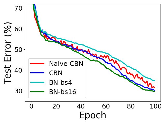
Figure 4. Training and test curves for CBN, Naive CBN, and BN
4.3. Ablation Study on ImageNet, with batch size per GPU of 4 and temporal window
Effect of temporal window size k. We conduct this ab- size k = 4 for CBN, Naive CBN, and BN-bs4, and batch size per
lation on ImageNet image classification and COCO object GPU of 16 for BN-bs16. The plot of BN-bs16 is the ideal bound.
detection, with each GPU processing 4 images. Figure 3
presents the results. When k = 1, only the batch from the network weights over iterations. Compared with the origi-
current iteration is utilized; therefore, CBN degenerates to nal BN upper bound, CBN achieves similar accuracy at the
the original BN. The accuracy suffers due to the noisy statis- same effective example number. This result indicates that
tics on small batch sizes. As the window size k increases, the compensation using a low-order Taylor polynomial by
more examples from recent iterations are utilized for statis- CBN is effective.
tics estimation, leading to greater accuracy. Accuracy satu- Figure 4 presents the train and test curves of CBN, Naive
rates at k = 8 and even drops slightly. For more distant it- CBN, BN-bs4, and BN-bs16 on ImageNet, with 4 images
erations, the network weights differ more substantially and per GPU and a temporal window size of 4 for CBN, Naive
Taylor polynomial approximation becomes less accurate. CBN, and BN-bs4, and 16 images per GPU for BN-bs16.
On the other hand, it is empirically observed that the The train curve of CBN is close to BN-bs4 at the beginning,
original BN saturates at a batch size of 16 or 32 for nu- and approaches BN-bs16 at the end. The reason is that we
merous applications [18, 31], indicating that the computed adopt a burn-in period to avoid the disadvantage of rapid
statistics become accurate. Thus, a temporal window size statistics change at the beginning of training. The gap be-
of k = min(d bs per16GPU e, 8) is suggested. tween the train curve of Naive CBN and CBN shows that
Effect of compensation. To study this, we compare Naive CBN cannot even converge well on the training set.
CBN to 1) Naive CBN, where statistics from recent itera- The test curve of CBN is close to BN-bs16 at the end, while
tions are directly aggregated without compensation via Tay- Naive CBN exhibits considerable jitter. All these phenom-
lor polynomial; and 2) the original BN applied with the ena indicate the effectiveness of our proposed Taylor poly-
same effective example number as CBN (i.e., its batch size nomial compensation.
per GPU is set to the product of batch size per GPU and Effect of burn-in period length T . We study the effect
temporal window size of CBN), which does not require any of varying the burn-in period length Tburn-in , at 4 images per
compensation and serves as an upper performance bound. GPU on both ImageNet image classification (ResNet-18)
The experimental results are also presented in Figure 3. and COCO object detection (Faster R-CNN with FPN and
CBN clearly surpasses Naive CBN when the previous itera- ResNet-50). Figure 5(a) and 5(b) present the results. When
tions are included. Actually, Naive CBN fails when the tem- the burn-in period is too short, the accuracy suffers. This
poral window size grows to k = 8 as shown in Figure 3(a), is because at the beginning of training, the network weights
demonstrating the necessity of compensating for changing change rapidly, causing the compensation across iterations
770
Memory FLOPs Training Inference
69 37.5 (GB) (M) Speed (iter/s) Speed (iter/s)
Top-1 accuracy
68
BN 14.1 5155.1 1.3 6.2
APbbox
67 37
66 GN 14.1 5274.2 1.2 3.7
36.5
65
CBN CBN
CBN 15.1 5809.7 1.0 6.2
64 BN 36 BN Table 8. Comparison of theoretical memory, FLOPs and practi-
63
10 20 30 40 50 60 70 80 90 1 3 5 7 9 11 cal training and inference speed between original BN, GN, and
Burn-in period (epoch) Burn-in period (epoch)
CBN in both training and inference on COCO.
(a) ImageNet (b) COCO
Figure 5. Results of different burn-in periods (in epochs) on BN Naive CBN CBN(1) CBN(2)
CBN, with batch size per iteration of 4, on ImageNet and COCO. Top-1 acc 65.1 66.8 70.0 70.0
Epoch-8 Epoch-9 Epoch-10 Epoch-11 Table 9. Top-1 accuracy of CBN that compensating with different
APbbox 37.7 37.7 37.6 37.3 orders and batch size per iter = 4 on ImageNet.
Table 7. Results on switching from BN to syncBN at different
epochs on COCO. From these results, the additional overhead of CBN is seen
to be minor. Also, merging BN/CBN into convolution in
to be less effective. When the burn-in period is too long, inference [12] could be utilized for further speedup.
i.e., CBN is involved too late and the overall performance Using second order statistics for compensation. Re-
drops to the BN baseline. sults of CBN with different orders of Taylor expansion
An interesting observation is that the accuracy is stable (batch size = 4, #iterations for approximation = 3) are shown
for a wide range of burn-in periods Tburn-in . This leads to in Table 9. By directly using the statistics of recent itera-
a question of whether BN in the small batch-size regime tions without compensation, Naive CBN outperforms BN
only suffers in terms of generalization performance in later with batch size 4 by 1.7% in accuracy. Via compensat-
stages of training. For further exploration, we design an ing the statistics of recent iterations with a first-order Tay-
experiment to remove other influences: we first train the lor expansion, CBN(1) can further improve the accuracy by
model on COCO with standard BN and a small batch size, 3.2% compared to Naive CBN. However, CBN(2) using a
then switch BN to syncBN. We present the experimental second-order approximation does not achieve better perfor-
results in Table 7. Results show that syncBN works simi- mance than CBN(1) . This may be because CBN(1) already
larly to CBN, which further verifies the high performance achieves performance comparable to BN with large batch
of CBN. It also supports our assumption that BN in the size, which serves as the upper bound of our approach, indi-
small batch-size regime only suffers in terms of general- cating that a first-order approximation is enough for image
ization performance in later stages of training, which may classification on ImageNet. Therefore, first-order compen-
shed some light on the small batch-size regime. sation for CBN is adopted by default.
Using more than one layer for compensation. We also
4.4. Analysis study the influence of applying compensation over more
than one layer. CBN using two layers for compensation
Computational cost, memory footprint, and train- achieves 70.1 on ImageNet (batch size per GPU=4, k=4),
ing/inference speed. We examine the computational cost, which is comparable to CBN using only one layer. How-
memory footprint, and the training and inference speed of ever, the efficient implementation can no longer be used
BN, GN and CBN in a practical COCO object detection task when more than one layer of compensation is employed. As
using R50-Mask R-CNN, shown in Table 8. The batch size using more layers does not further improve performance but
per GPU and window size of CBN are set to 4. consumes more FLOPs, we adopt one-layer compensation
Compared to BN and GN, CBN consumes about 7% for CBN in practice.
extra memory and 11% more computational cost. The
extra memory mainly contains the statistics (µ and ν),
5. Conclusion
their respective gradients, and the network parameters
(θt−1 · · · θt−(k−1) ) of previous iterations, while the com- In the small batch size regime, batch normalization is
putational cost comes from calculations of the statistics’ widely known to drop dramatically in performance. To
respective gradients, Taylor compensations, and averaging address this issue, we propose to enhance the quality of
operations. statistics via utilizing examples from multiple recent iter-
The overall training speed of CBN is close to both BN ations. As the network activations from different iterations
and GN. It is worth noting that the inference speed of CBN are not comparable to each other due to changes in network
is equal to BN, which is much faster than GN. The inference weights, we compensate for the network weight changes
stage of CBN is the same as that of BN, where pre-recorded based on Taylor polynomials, so that the statistics can be
statistics can be used instead of online statistics calculation. accurately estimated. In the experiments, the proposed ap-
8proach is found to outperform original batch normalization [13] Tsung-Yi Lin, Piotr Dollar, Ross Girshick, Kaiming He,
and a direct calculation of statistics over previous iterations Bharath Hariharan, and Serge Belongie. Feature pyramid
without compensation. Moreover, it achieves performance networks for object detection. In The IEEE Conference
on par with SyncBN, which can be regarded as the upper on Computer Vision and Pattern Recognition (CVPR), July
bound, on both ImageNet and COCO object detection. 2017. 6
[14] Tsung-Yi Lin, Michael Maire, Serge Belongie, James Hays,
Pietro Perona, Deva Ramanan, Piotr Dollár, and C Lawrence
References Zitnick. Microsoft coco: Common objects in context. In
European conference on computer vision, pages 740–755.
[1] Jimmy Lei Ba, Jamie Ryan Kiros, and Geoffrey E Hin-
Springer, 2014. 6
ton. Layer normalization. arXiv preprint arXiv:1607.06450,
[15] Jonathan Long, Evan Shelhamer, and Trevor Darrell. Fully
2016. 1, 2
convolutional networks for semantic segmentation. In Pro-
[2] Liang-Chieh Chen, George Papandreou, Iasonas Kokkinos, ceedings of the IEEE conference on computer vision and pat-
Kevin Murphy, and Alan L Yuille. Deeplab: Semantic image tern recognition, pages 3431–3440, 2015. 1
segmentation with deep convolutional nets, atrous convolu-
[16] Ping Luo, Jiamin Ren, and Zhanglin Peng. Differentiable
tion, and fully connected crfs. IEEE transactions on pattern
learning-to-normalize via switchable normalization. arXiv
analysis and machine intelligence, 40(4):834–848, 2017. 1
preprint arXiv:1806.10779, 2018. 2, 7
[3] Jifeng Dai, Haozhi Qi, Yuwen Xiong, Yi Li, Guodong [17] Hyeonseob Nam and Hyo-Eun Kim. Batch-instance nor-
Zhang, Han Hu, and Yichen Wei. Deformable convolutional malization for adaptively style-invariant neural networks. In
networks. In Proceedings of the IEEE international confer- Advances in Neural Information Processing Systems, pages
ence on computer vision, pages 764–773, 2017. 1 2563–2572, 2018. 2
[4] Kaiming He, Georgia Gkioxari, Piotr Dollár, and Ross Gir- [18] Chao Peng, Tete Xiao, Zeming Li, Yuning Jiang, Xiangyu
shick. Mask r-cnn. In Proceedings of the IEEE international Zhang, Kai Jia, Gang Yu, and Jian Sun. Megdet: A large
conference on computer vision, pages 2961–2969, 2017. 6, mini-batch object detector. In Proceedings of the IEEE Con-
7 ference on Computer Vision and Pattern Recognition, pages
[5] Kaiming He, Xiangyu Zhang, Shaoqing Ren, and Jian Sun. 6181–6189, 2018. 1, 2, 7
Deep residual learning for image recognition. arXiv preprint [19] Siyuan Qiao, Huiyu Wang, Chenxi Liu, Wei Shen, and
arXiv:1512.03385, 2015. 5 Alan Yuille. Weight standardization. arXiv preprint
[6] Kaiming He, Xiangyu Zhang, Shaoqing Ren, and Jian Sun. arXiv:1903.10520, 2019. 2
Deep residual learning for image recognition. In Proceed- [20] Shaoqing Ren, Kaiming He, Ross Girshick, and Jian Sun.
ings of the IEEE conference on computer vision and pattern Faster r-cnn: Towards real-time object detection with region
recognition, pages 770–778, 2016. 2, 6 proposal networks. In Advances in neural information pro-
[7] Tong He, Zhi Zhang, Hang Zhang, Zhongyue Zhang, Jun- cessing systems, pages 91–99, 2015. 1, 6, 7
yuan Xie, and Mu Li. Bag of tricks for image classification [21] Olga Russakovsky, Jia Deng, Hao Su, Jonathan Krause, San-
with convolutional neural networks. In The IEEE Confer- jeev Satheesh, Sean Ma, Zhiheng Huang, Andrej Karpathy,
ence on Computer Vision and Pattern Recognition (CVPR), Aditya Khosla, Michael Bernstein, et al. Imagenet large
June 2019. 5 scale visual recognition challenge. International journal of
computer vision, 115(3):211–252, 2015. 2, 5
[8] Gao Huang, Zhuang Liu, Geoff Pleiss, Laurens Van
[22] Tim Salimans and Diederik P Kingma. Weight normaliza-
Der Maaten, and Kilian Weinberger. Convolutional networks
tion: A simple reparameterization to accelerate training of
with dense connectivity. IEEE transactions on pattern anal-
deep neural networks. In Advances in Neural Information
ysis and machine intelligence, 2019. 6
Processing Systems, pages 901–909, 2016. 2
[9] Sergey Ioffe. Batch renormalization: Towards reducing
[23] Mark Sandler, Andrew Howard, Menglong Zhu, Andrey Zh-
minibatch dependence in batch-normalized models. In Ad-
moginov, and Liang-Chieh Chen. Mobilenetv2: Inverted
vances in Neural Information Processing Systems, pages
residuals and linear bottlenecks. In Proceedings of the
1945–1953, 2017. 1, 2, 5
IEEE conference on computer vision and pattern recogni-
[10] Sergey Ioffe and Christian Szegedy. Batch normalization: tion, pages 4510–4520, 2018. 6
Accelerating deep network training by reducing internal co- [24] Wenqi Shao, Tianjian Meng, Jingyu Li, Ruimao Zhang,
variate shift. In International Conference on Machine Learn- Yudian Li, Xiaogang Wang, and Ping Luo. Ssn: Learn-
ing, pages 448–456, 2015. 1, 2, 3, 5 ing sparse switchable normalization via sparsestmax. arXiv
[11] Yann LeCun, Léon Bottou, Genevieve B Orr, and Klaus- preprint arXiv:1903.03793, 2019. 2
Robert Müller. Efficient backprop. In Neural Networks: [25] K. Simonyan and A. Zisserman. Very deep convolu-
Tricks of the Trade, this book is an outgrowth of a 1996 NIPS tional networks for large-scale image recognition. CoRR,
workshop, pages 9–50. Springer-Verlag, 1998. 2 abs/1409.1556, 2014. 6
[12] Dawei Li, Xiaolong Wang, and Deguang Kong. Deeprebirth: [26] J Sola and Joaquin Sevilla. Importance of input data nor-
Accelerating deep neural network execution on mobile de- malization for the application of neural networks to complex
vices. In Proceedings of the AAAI Conference on Artificial industrial problems. IEEE Transactions on nuclear science,
Intelligence, volume 32, 2018. 8 44(3):1464–1468, 1997. 2
9[27] Christian Szegedy, Sergey Ioffe, Vincent Vanhoucke, and
Alexander A Alemi. Inception-v4, inception-resnet and the
impact of residual connections on learning. In Thirty-first
AAAI conference on artificial intelligence, 2017. 6
[28] Dmitry Ulyanov, Andrea Vedaldi, and Victor Lempitsky. In-
stance normalization: The missing ingredient for fast styliza-
tion. arXiv preprint arXiv:1607.08022, 2016. 1, 2
[29] Guangrun Wang, Ping Luo, Xinjiang Wang, Liang Lin, et al.
Kalman normalization: Normalizing internal representations
across network layers. In Advances in Neural Information
Processing Systems, pages 21–31, 2018. 2
[30] Xiaolong Wang, Ross Girshick, Abhinav Gupta, and Kaim-
ing He. Non-local neural networks. In Proceedings of the
IEEE Conference on Computer Vision and Pattern Recogni-
tion, pages 7794–7803, 2018. 1
[31] Yuxin Wu and Kaiming He. Group normalization. In Pro-
ceedings of the European Conference on Computer Vision
(ECCV), pages 3–19, 2018. 1, 2, 5, 6, 7
10A. Algorithm Outline and θl denote µlt−τ (θt−τ ) and θt−τ
l
respectively, by remov-
ing the irrelevant notations for iterations. The element-wise
Algorithm 1 presents an outline of our proposed Cross- computation in the forward pass can be computed as
Iteration Batch Normalization (CBN).
m
1 X l
Algorithm 1: Cross-Iteration Batch Normaliza- µlj = x , (13)
m i=1 i,j
tion(CBN)
Input: Feature responses of a network node of the where µlj denotes the j-th channel in µl , and xli,j denotes
l-th layer at the t-th iteration {xlt,i (θt )}m i=1 , the j-th channel in the i-th example. xli,j is computed as
network weights {θt−τ l
}k−1
τ =0 , statistics
{µlt−τ (θt−τ )}k−1 l
τ =1 and {νt−τ (θt−τ )}τ =1 ,
k−1 Cin X
X K
l−1
and gradients {∂µt−τ (θt−τ )/∂θt−τ l
}k−1 xli,j = l
θj,n,k · yi+offset(k),n , (14)
τ =1
l k−1 n=1 k=1
and {∂νt−τ (θt−τ )/∂θt−τ }τ =1 from most
recent k − 1 iterations where n and k enumerate the input feature dimension and
l
Output: {yt,i (θt ) = CBN(xlt,i (θt ))} the convolution kernel index, respectively, offset(k) denotes
1
Pm
1 µt (θt ) ← m xt,i (θt ), the spatial offset in applying the k-th kernel, and y l−1 is the
1
Pi=1
m
νt (θt ) ← m i=1 x2t,i (θt ) //statistics on the output of the (l − 1)-th layer.
current iteration The element-wise calculation of ∂µl /∂θl ∈
2 for τ ∈ {1, . . . , k} do Cout ×Cout ×Cin ×K
R is as follows, taking Eq. (13) and
3 µlt−τ (θt ) ← Eq. (14) into consideration:
∂µl (θ )
µlt−τ (θt−τ ) + t−τ t−τ l
(θtl − θt−τ ) ∂µlj
l
∂θt−τ ∂µl
//approximation from recent iterations [ ]j,q,p,η =
∂θl l
∂θq,p,η
l l ∂ν l (θ )
4 νt−τ (θt ) ← νt−τ (θt−τ )+ t−τ l
t−τ l
(θtl −θt−τ ) 1
Pm l
∂θt−τ ∂m i=1 xi,j
//approximation from recent iterations = l
∂θq,p,η
5 end Pm PCin PK l
1 l−1
∂ m i=1 n=1 k=1 θj,n,k · yi+offset(k),n
Pk−1
6 µ̄lt,k (θt ) ← k1 τ =0 µlt−τ (θt ) //averaging over
= l
recent iterationsPk−1 ∂θq,p,η
(θt ) ← k1 τ =0 max νt−τ
l
l
7 ν̄t,k (θt ), µlt−τ (θt )2 1 Pm l−1
m i=1 yi+offset(η),p , j=q
//validation and averaging over recent iterations = .
8
l
σ̄t,k (θt )2 ← ν̄t,k
l
(θt ) − µ̄lt,k (θt )2 0 , j 6= q
xlt,i (θt )−µ̄lt,k (θt )
(15)
9 x̂lt,i (θt ) = q
l (θ )2 +
//normalize
σ̄t,k t l
10
l
yt,i (θt ) ← γ x̂lt,i (θt ) + β //scale and shift Thus, [ ∂µ ]
∂θ l j,q,p,η
takes non-zero values only when j = q.
This operation can be implemented efficiently in O(Cin ×
K). Similarly, the calculation of ∂ν l /∂θl can be obtained
in O(Cout × Cin × K).
B. Efficient Implementation of
∂µlt−τ (θt−τ )/∂θt−τ
l l l
and ∂νt−τ (θt−τ )/∂θt−τ C. Observation of the gradients diminishing
Let Cout and Cin denote the output and input channel The key assumption in Eq. (7) and Eq. (8) is that for
dimension of the l-th layer, respectively, and K denotes the a node at the l-th layer, the gradient of its statistics with
l
kernel size of θt−τ . µlt−τ and νt−τ
l
are thus of Cout dimen- respect to the network weights at the l-th layer is larger than
l
sions in channels, and θt−τ is a Cout ×Cin ×K dimensional that of weights from the prior layers, i.e.,
tensor. A naive implementation of ∂µlt−τ (θt−τ )/∂θt−τ l
l l
and ∂νt−τ (θt−τ )/∂θt−τ involves computational overhead ||gµ (l|l, t, τ )||F
||gµ (r|l, t, τ )||F
of O(Cout × Cout × Cin × K). Here we find that the ||gν (l|l, t, τ )||F
||gν (r|l, t, τ )||F , r(a) The gradients of µ (b) The gradients of ν
Figure 6. Comparison of gradients of statistics w.r.t. current layer
vs. that w.r.t. previous layers on ImageNet.
||gµ (r)||F /||gµ (l)||F and ||gν (r)||F /||gν (l)||F for r ∈ {l −
1, l − 2} are averaged over all CBN layers of the network
at different training epochs (Figure 6). The results suggest
that the key assumption holds well, thus validating the ap-
proximation in Eq. (7) and Eq. (8).
We also study the gradients of non-ResNet models. The
ratios of ||gµ ||F and ||gν ||F are (0.20 and 0.41) for VGG-
16 and (0.15 and 0.37) for Inception-V3, which is similar
to ResNet (0.12 and 0.39), indicating that the assumption
should also hold for the VGG and Inception series.
12You can also read