Faster Genetic Programming GPquick via multicore and Advanced Vector Extensions
←
→
Page content transcription
If your browser does not render page correctly, please read the page content below
RN/19/01                                                                                    Research
                                         23 February 2019                                                                               Note

                                                                Faster Genetic Programming GPquick
                                                            via multicore and Advanced Vector Extensions
arXiv:1902.09215v1 [cs.NE] 25 Feb 2019

                                                            William B. Langdon (UCL) and Wolfgang Banzhaf (MSU)

                                                                              Fax: +44 (0)20 7679 1397

                                                                                      Abstract

                                              We evolve floating point Sextic polynomial populations of genetic programming binary trees
                                              for up to a million generations. Programs with almost 400 000 000 instructions are created
                                              by crossover. To support unbounded Long-Term Evolution Experiment LTEE GP we use
                                              both SIMD parallel AVX 512 bit instructions and 48 threads to yield performance of up to
                                              139 billion GP operations per second, 139 giga GPops, on a single Intel Xeon Gold 6126
                                              2.60 GHz server.

                                                                                                 Department of Computer Science
                                                                                                 University College London
                                                                                                 Gower Street
                                                                                                 London WC1E 6BT, UK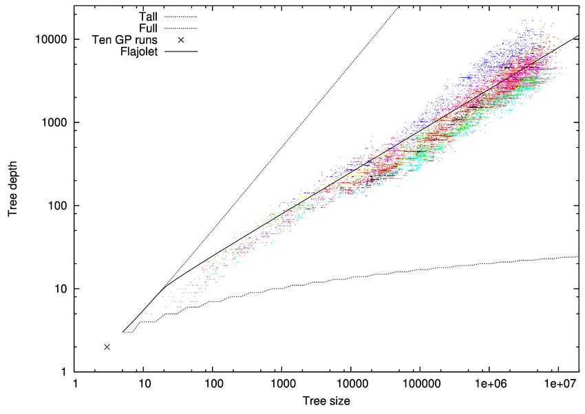
0.1

                                                                                                                     2161
                                                                                                                             3603

                   Best fitness = Mean |error| 48 fixed test cases
                                                                                                              1294
                                                                                                                    1640
                                                                       0.01
                                                                                                                   793

                                                                      0.001
                                                                                                            397      1886
                                                                                                                       619

                                                                                                                        2055
                                                                     0.0001

                                                                                                                      1753

                                                                              1   10   100           1000              10000
                                                                                        Generation                1.11334e-09

Figure 1: Evolution of mean absolute error in ten runs of Sextic polynomial Koza (1992) with population
of 4000. (Runs aborted after first crossover to hit 15 million node limit.) End of run label gives number of
generations when fitness got better (five shown at top right to avoid crowding).

keywords: genetic algorithms, genetic programming, GP, Convergence, Long-Term Evolution Experiment
LTEE Extended unbounded evolution

1       Introduction

A couple of years we noted Langdon (2017) Rich Lenski’s experiments in long term evolution Lenski
et al. (2015) in which the BEACON team evolved bacteria for more than 70 000 generations and found
continued beneficial adaptive mutations. This prompted us to ask the same question in computation based
evolution. We started to investigate what happens if we allow artificial evolution, specifically genetic
programming (GP) with crossover Koza (1992); Banzhaf et al. (1998); Poli et al. (2008), to evolve for tens
of thousands, even a hundred thousand generations. Since then new hardware has become available and
we build a new GP engine based on Andy Singleton’s GPQUICK (Section 2). This allows us to switch
from the Boolean to the continuous domain and run experiments of up to a million generations. Excluding
some special applications or Boolean benchmarks based on graphics hardware (GPUs), at up to 139 billion
GP operations per second (139 giga GPops), this appears to be the fastest single computer GP system
(Langdon, 2013, Tab. 3).

In the Boolean domain we found usually the population quickly found a best possible answer and then re-
tained it exactly for thousands of generations. Nonetheless under subtree crossover we reported interesting
population evolution with trees continuing to evolve. Indeed we were able to report the first signs of an
eventual end of bloat due to fitness convergence of the whole population. We can now report in the con-
tinuous domain we do see (like the bacteria experiments) continual innovation and improvement in fitness.
Figure 1 show that although the rate of innovation falls (as in Lenski’s E. Coli1 populations), typically
better solutions are found even towards the end of the runs and, in these runs, there are several hundred or
even a few thousand generations where sub-tree crossover between evolved parents gave a better child.

    1
        The E. Coli genome contains 4.6 million DNA base pairs.

                                                                                       1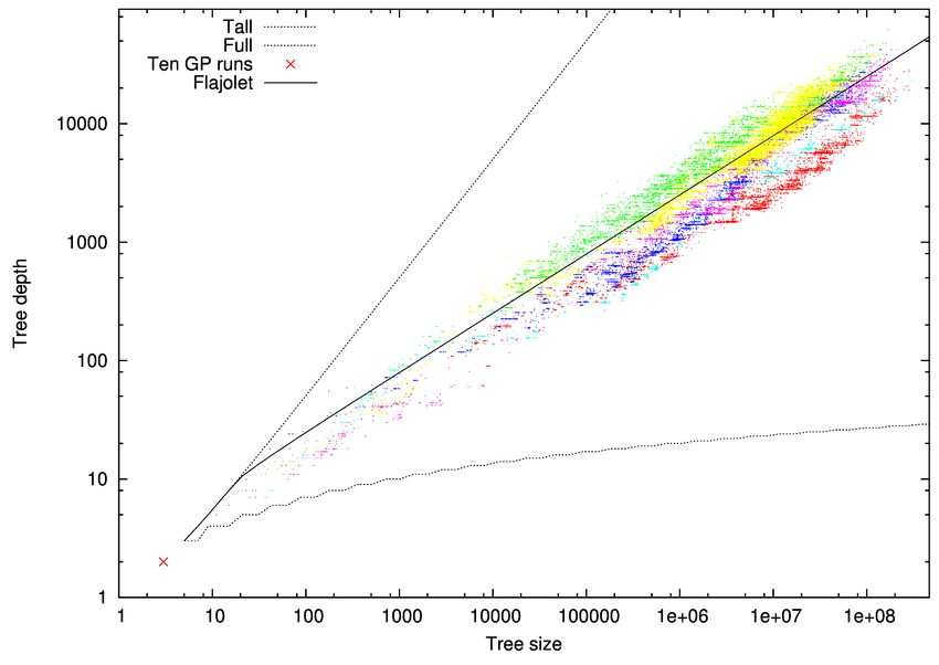
We are going to run GP far longer than is normally done. Firstly in search of continual evolution but also
noting that it is sometimes not safe to extrapolate from the first hundred or so generations. As an example,
McPhee (McPhee and Poli, 2001, sect. 1.2) said that his earlier studies which had reported only the first
100 generations could not safely be extrapolated to 3000 generations.

It must be admitted that without size control we expect bloat2 , and so we need a GP system not only able
to run for 106 generations3 but also able to process trees with well in excess of a 100 million nodes4 . The
new system we use is based on Singleton’s GPQuick Singleton (1994); Keith and Martin (1994); Langdon
(1998) but enhanced to take advantage of both multi-core computing using pthreads and Intel’s SIMD AVX
parallel floating point operations (Section 2). Keith and Martin (1994) say GPQuick’s linearisation of the
GP tree will be hard to parallelise. Nevertheless, GPQUICK was rewritten to use 16 fold Intel AVX-512
instructions to do all operations on each node in the GP tree immediately. Leading to a single eval pass and
better cache locality but at the expense of keeping a T = 48 wide stack of partial results per thread.

Although the populations never lose genetic diversity (Koza’s variety Koza (1992)), with strong tournament
selection (parent selection tournaments of size seven, see Table 1) even the larger populations do tend to
converge to have identical fitness values. However 100% fitness convergence is only seen in long runs with
smaller populations (500 or 48 trees). In contrast, in the Boolean domain Langdon (2017), even in bigger
populations (500) there are many generation where the whole population has identical fitness (but again
variety is 100%).

The next section describes how GPQUICK was adapted to take advantage of Intel SIMD instructions
able to process 16 floating point numbers in parallel and Posix threads to perform crossover and fitness
evaluation on 48 cores simultaneously. Section 3 describes the floating point benchmark (Table 1 and
Figure 4). Whilst Section 4 describes the evolution of fitness, size and depth in populations of 4000, 500
and 48 trees.
         p     It finds the earlier predictions of sub-quadratic bloat Langdon (1999a) and Flajolet limit
(depth ≈ 2π|size| Langdon (2000b)) to essentially hold. In Section 5 there is a short discussion about the
continuous evolution permitted by floating point benchmarks before we conclude in Section 6.

2       GPQUICK

First we describe how GPQUICK is used with the Sextic polynomial regression problem and then how
GPQUICK has been modified to run in parallel, Sections 2.2 and 2.3.

2.1      Sextic and GPQuick

Andy Singleton’s GPQUICK Singleton (1994) is a well established fast and memory efficient C++ GP
framework. In steady state mode Syswerda (1990) it stores GP trees in just one byte per tree node. (Orig-
inally it supported only steady state GAs. Ages ago a quick conversion to support generational GAs, with
separate parent and child populations doubled this, although Koza (1992) shows doubling is not necessary.)
The 8 bit opcode per tree node allows GPQUICK to support a number of different functions and inputs.
Typically (as in these experiments) the remaining opcodes are used to support about 250 fixed ephemeral
    2
     GP’s tendency to evolve non parsimonious solutions has been known since the beginning of genetic program-
ming. E.g. it is mentioned in Jaws (Koza, 1992, page 7). Walter Tackett (Tackett, 1994, page 45) credits Andrew
Singleton with the theory that GP bloats due to the cumulative increase in non-functional code, known as introns.
The theory says these protect other parts of the same tree by deflecting genetic operations from the functional code
by simply offering more locations for genetic operations. The bigger the introns, the more chance they will be hit by
crossover and so the less chance crossover will disrupt the useful part of the tree. Hence bigger trees tend to have
children with higher fitness than smaller trees. See also Altenberg (1994); Angeline (1994). In Langdon (2017) we
showed prolonged evolution can produce converged populations of functionally identical but genetically different
trees comprised of the same central core of functional code next to the root node plus a large amount of variable
ineffective sacrificial code.
    3
     The median run shown in Figure 2 took 39 hours (mean 62 hours).
    4
      Again referring to the extended runs in Figure 2, crossover creates highly evolved trees containing almost four hundred
million nodes These are by far the largest programs yet evolved.

                                                             2
Figure 2: 11 extended runs pop=48. Numbers on right indicate size of largest tree before the run stopped in
millions of nodes. One run (*) converged so that more than 90% of the trees contain just five nodes. Three
of the other four runs that reached 1 million generations (red) took between half a day and five days. In all
but one run (*) we see repeated substantial bloat (> 64 million nodes) and subsequent tree size collapse.
Seven runs, in black, terminated due to running out of memory (on server with 46GB).
Figure 3: Size and convergence in last 20% of a typical extended run pop=48. (First run “64” in Figure 2.)
Solid blue curve shows almost all the time there are less than 2 trees with the maximum fitness (rescaled
by ×5 106 and smoothed over 30 generations). In populations with huge trees, there are many generations
where the whole population has identical fitness. Without a fitness differential, tree size may rise or fall.
3random constants Poli et al. (2008). In the Sextic polynomial we have the traditional four binary floating
point operations (+, −, × and protected division), an input (x) and 250 constants. The constants are chosen
at random from the 2001 floating point numbers from -1.000 to +1.000. By chance neither end point nor
0.000 were chosen (see Table 1).
The continuous test cases (x) are selected at random from the interval -1 to +1. At the same time the target
value y is calculated (Table 1). Since both x and y are stored in a text file, there may be slight floating point
rounding errors from the standard float⇔string conversions.
Whereas the Sextic polynomial is usually solved with 50 test cases Langdon et al. (1999), since the AVX
hardware naturally supports multiples of 16, in our experiments we change this to 48 (i.e. 3 × 16) (Table 1).
The multi-core servers we use each support 48 threads and for in the longest extended runs, we reduce the
population to 48 (whereas in Langdon (2017) the smallest population considered contained 50 trees).
2.2 AVX GPQuick
GPQUICK stores the GP population by flattening each tree into a linear buffer, with the root node at
the start. To avoid heap fragmentation the buffers are all of the same size. Traditionally the buffer is
interpreted once per test case by multiple recursive calls to EVAL and the tree’s output is retrieved from
the return value of the outer most EVAL. Each nested EVAL moves the instruction pointer on one position
in the tree’s buffer, decodes the opcode there and calls the corresponding function. In the case of inputs x
and constants a value is returned via EVAL immediately, whereas ADD, SUB, MUL and DIV will each
call EVAL twice to obtain their arguments before operating on them and returning the result. For speed
GPQUICK’s FASTEVAL, does an initial pass though the buffer and replaces all the opcodes by the address
of the corresponding function that EVAL would have called. This expands the buffer 16 fold, but the
expanded buffer is only used during evaluation and can be reused by every member of the population. Thus
originally EVAL processed the tree T + 1 times (for T test cases).
The Intel AVX instructions process up to 16 floating point data simultaneously. The AVX version of EVAL
was rewritten to take advantage of this. Indeed as we expect trees that are far bigger than the CPU cache
(≈16 million bytes, depending on model), EVAL was rewritten to process each tree’s buffer only once.
This is achieved by EVAL processing all of the test cases for each opcode, instead of processing the whole
of the tree on one test case before moving on to the test case. Whereas before each recursive call to EVAL
returned a single floating point value, now it has to return 48 floating point values. This was side stepped
by requiring EVAL to maintain an external stack where each stack level contains 48 floating point values.
The AVX instructions operate directly on the top of this stack and EVAL keeps track of which instruction
is being interpreted, where the top of the stack is, and (with PTHREADS) which thread is running it. Small
additional arrays are used to allow fast translation from opcode to address of eval function, and constant
values. AVX instructions are used to speed loading each constant into the top stack frame. Similarly all
48 test cases (x) are rapidly loaded on to the top of the stack. However the true power comes from being
able to use AVX to process the top of the stack and the adjacent stack frame (holding a total of 96 floats)
in essentially three instructions to give 48 floating point results.
The depth of the evaluation stack is simply the depth of the GP tree. GPQUICK uses a fixed buffer length
for everyone in the GP population. This is fixed by the user at the start of the GP run. Fixing the buffer size
also sets the maximum tree size. Although in principle this only places a very weak limit on GP tree depth,
it has been repeatedly observed Langdon (1999c, 2000b) that evolved trees are roughly shaped like random
trees. The mathematics of trees is well p studied Sedgewick and Flajolet (1996) in particular the depth of
random binary trees tends to a limit 2 πdtreesize/2e + O(tree size 1/4+ ) (Sedgewick and Flajolet, 1996,
page 256). (See Flajolet limit in Figures 6, 7, 11 and 15.) Thus the user specified tree size limit can be
readily converted into an expected maximum depth of evolved trees. The size of the AVX eval stack is set
to this plus a suitable allowance for random fluctuations and O(tree size1/4+ ). Note, with very large trees,
even allowing for the number of test cases and storing floats on the stack rather than byte sized opcodes,
the evaluation stack is considerably smaller than the genome of the tree whose fitness it is calculating.
4Although AVX allows reductions operations across a stack frame, these are not needed until the final
conversion from output to fitness value. However although faster, the reduction operations manipulate the
48 numbers in a different order and so may (within floating point tolerances) produced different answers.
Since the reduction is a tiny part of the whole fitness evaluation we decided instead to ensure the AVX
version produces identical results to the original system and so the final fitness evaluation is done with a
conventional for loop.
2.3 PTHREADS GPquick
The second major change to GPQUICK was to delay fitness evaluation so that the whole new population
can have its fitness evaluated in parallel. (This means PTHREADS can only be applied when GPQUICK
is operating in generational mode.) If pThreads > 0, the population fitness evaluation is spread across
pThreads. As trees are of different sizes, each fitness evaluation will take different times. Therefore which
tree is evaluated by which thread is decided dynamically. Due to timing variations, in an identical run,
which tree is evaluated by which thread may be different. However great care is taken so that this cannot
effect the course of evolution. (Although, for example, where trees have identical fitness, it can affect
which is found first and therefore which is reported to the user).
EVAL requires a few data arrays. These are all allocated near the start of the GP run. Those that are read
only can be shared by the threads. Each thread requires its own instance of read-write data. To avoid “false
sharing”, care is taken to align read-write data on cache line boundaries (64 bytes), e.g. with additional
padding bytes and ((aligned)). So that each thread writes to its own cache lines and therefore these
cached data are not shared with other threads.
Surprisingly an almost doubling of speed was obtained by also moving crossover operations to these par-
allel threads. Since crossover involves random choices of parents and subtrees these were unchanged but
instead of performing the crossover immediately a small amount of additional information was retained
and to be read later by the threads. This allows the crossover to be delayed and performed in one of 48 C++
pthreads. The results are identical but give and additional ≈two fold speed up.
With intermediate sized trees, there may be some efficiency gain by evaluating the newly created chromo-
some immediately (i.e. whilst still in the hardware cache).
One thing that was less successful was to implement a strategy for minimising memory consumption
by deleting parents immediately all their children have been created. (Koza’s generational scheme with
crossover means at most M + 2 individuals need to be stored (where M is the population size). In prin-
ciple this grows to M + 2t (where t is the number of threads). This of course gives no saving where the
population is the same size or smaller than the number of threads. Although getting the threads to free
memory immediately works, C++ free is surprisingly slow in a multi-threaded environment (within threads
it has to wait on locks to avoid corrupting its heap). This seriously impacted performance (unless the time
taken by EVAL dominates). Therefore the calls to delete parents were moved back out of the threads to the
surrounding sequential code.
In principle, even with multiple threads t > 1, the efficient reduction of memory from 2M to M + 2t
chromosomes should be possible. The number and size of all buffers is known in advance and it would be
possible to manipulate the allocation and freeing explicitly in GPQUICK’s chrome.cxx C++ source directly
(rather than using new and delete). Thus effectively building a specialised heap for the population but this
has not been attempted.
3 Experiments
We use the well known Sextic polynomial benchmark (Koza, 1994, Tab. 5.1). Briefly the task given to
GP is to find an approximation to a sixth order polynomial, x6 − 2x4 + x2 , given only a fixed set of
samples. I.e. a fixed number of test cases. For each test input x we know the anticipated output f (x), see
50.16
0.14
0.12
0.1
0.08
f(x)
0.06
0.04
0.02
0
-0.02
-1 -0.8 -0.6 -0.4 -0.2 0 0.2 0.4 0.6 0.8 1
x
Figure 4: 48 test cases for Sextic Polynomial Benchmark.
Table 1: Long term evolution of Sextic polynomial symbolic regression binary trees
Terminal set: X, 250 constants -0.995 to 0.997
Function set: MUL ADD DIV SUB
Fitness cases:48 fixed input -0.97789 to 0.979541 (randomly selected from -1.0 to +1.0 input).
y = xx(x−1)(x−1)(x+1)(x +1)
1 P48
Selection: tournament size 7 with fitness = 48 i=1 |GP (xi ) − yi |
Population: Panmictic, non-elitist, generational.
Parameters: Initial population (4000) ramped half and half Koza (1992) depth between 2 and 6. 100% un-
biased subtree crossover. 10 000 generations (stop run if any tree reaches limit 15 106 ).
DIV is protected division (y!=0)? x/y : 1.0f
Figure 4 and Table 1. Of course the real point is to investigate how GP works. How GP populations evolve
over time. In particular, even for such a simple continuous problem, it is possible for GP to continue to
find improvements (as Lenski’s E.Coli are doing) or, like the Boolean case Langdon (2017), will the GP
population get stuck early on and from then on never make further progress?
We ran three sets of experiments. In the first the new GP systems was set up as like the original Sextic
polynomial runs which reported phenotypic convergence (Langdon et al., 1999, Fig. 8.5). The first group
use a population of 5000, the next 500 and the last 48. (Section 2.1 above has already described a few
technical differences between these and our earlier experiments Langdon et al. (1999).)
3.1 Crossover
Each generation is created entirely using Koza’s two parent subtree crossover Koza (1992). (GPQuick
creates one offspring per crossover.) For simplicity and in the hope that this would make GP populations
easier to analyse, both subtrees (i.e. to be removed and to be inserted) are chosen uniformly at random.
That is, we do not use Koza’s bias in favour of internal nodes (functions) at the expense of external nodes
(leafs or inputs). Instead the root node of the subtree (to be deleted or to be copied) is chosen uniformly
at random from the whole of the parent tree. This means there is more chance of subtree crossover simply
moving leaf nodes and so many children will differ from the root node donating parent (the mum) by just
one leaf.
6As mentioned above (Section 2.3) once fitness evaluation has been sped up by parallel processing, for very
long trees, producing the child is surprisingly large part of the remaining run time and so it too can be done
in parallel. However the choice of crossover points is done in the usual way (i.e. in sequential code, not
done in parallel) and so remains unaffected by multithreading. This ensures the variability introduced by
multiple parallel threads does not change the course of evolution.
3.2 Fitness Function
The fitness of every member of every generation is calculated using the same fitness function as That is,
baring rounding errors (page 4), fitness is given by the mean of the absolute difference between the value
returned by the GP tree on each test case and the Sextic polynomial’s value for the same test input (see
Table 1). However unlike Koza, we use tournament selection to chose both parents.
Like (Koza, 1994, Tab. 5.1), we also keep track of the number of test case where each tree is close to the
target (i.e. within 0.01, known as a “hit”). The number of hits is used for reporting the success of a GP run.
It is not used internally during a GP run. Also our GP runs do not stop when a solution is found (48 hits)
but continue until either the user specified number of generations is reached or bloat means the GP runs out
of memory.
Where needed, floating point calculations are done in a fixed order, to avoid parallelism creating minor
changes in calculated fitness, which could quickly cause otherwise identical runs to diverge because of
implementation differences in parallel calculations. (Also mentioned above above in Section 2.2.)
4 Results
4.1 Results Population 4000 trees
In the first set of experiments, we use the standard population of 4000 trees. Table 2 summarises the results
of 10 runs. In all cases GP found a reasonable approximation to the target (the Sextic polynomial). Indeed
in all but one run (47 hits) the best trees score 48 out of 48 possible hits. I.e. they are within 0.01 on all
48 test cases. Indeed in most cases the average error was less than 10−4 . Figure 1 shows that GP tends
to creep up on the best match to the training data. Typically after several thousand generations, GP has
progressively improved by more than a thousand increasingly small steps. (See Table 2 column 3 and
Figure 1).
In all cases we do see enormous increases in size. In all ten runs with a population of 4000, the runs are
stopped as they hit the size limit (15 000 000) before reaching 10 000 generations. Column 5 in Table 2
gives the size (in millions) of the largest evolved tree in each run. The log-log plot in Figure 5 shows a
typical pattern of sub quadratic Langdon (2000a) increase in tree size. The straight line, shows a power
law fit. In this run the best fit has an exponent of 1.2. Column 6 of Table 2 shows that the best fit between
generations ten and a thousand for all 10 runs varies between 1.1 and 1.9.
As expected not only do programs evolve to be bigger but also they increase in depth. As described above
(in Section 2.2) highlypevolved trees tend to be randomly shaped and so as expected tend to lie near the
Flajolet limit, depth ≈ 2π|size| (see Figures 6 and 7).
In all ten runs we see some phenotypic convergence. The last column in Table 2 shows the peak fitness
convergence. That is, out of 4000, the number of trees having exactly the same fitness as the best in the
population. Typically at the start of the run (see Figure 8), the population contains mostly poorer trees,
but later in the run the population begins to converge and towards the end of the run we may see hundreds
of generations where more than 90% of the population have identical fitness. Under these circumstances,
even with a tournament size as high as 7, many tournaments include potential parents with identical fitness.
These, and hence the parents of the next generation, are decided entirely randomly. However, even in
the most converged population there are at least two individuals with worse fitness. (In Figure 8 it is at
least 19.) As we saw with the Boolean populations Langdon (2017), even this small number can be enough
to drive bloat (albeit at a lower rate).
7Table 2: 10 Sextic polynomial runs with population 4000
Gens smallest error impr5 hits size106 power law conv
6370 0.000064487 2139 48 14.329 1.200 3981
8298 0.000145796 2040 48 14.102 1.916 3982
2323 0.000642006 389 47 13.441 1.387 3995
7119 0.000507600 608 48 13.668 1.589 3997
11750 0.000000001 3583 48 13.854 1.364 3989
3412 0.000065562 1277 48 14.348 1.625 3986
5106 0.000071289 1615 48 14.233 1.146 3988
6112 0.000728757 1871 48 14.500 1.254 3983
6679 0.000028853 1741 48 14.022 1.396 3998
4454 0.000067817 790 48 14.900 1.227 3997
5 Figure1 gives number of generations which improve on their parents, whereas here we give strictly better
than anything previously evolved. Hence slight differences.
1e+07
x^1.2
Mean Program size
1e+06
100000
10000
1000
100
10
1
1 10 100 1000 10000
Generation
Figure 5: Evolution of tree size in first Sextic run (population 4000). (This run aborted after 6370 gen-
erations by first crossover to hit 15 million node limit.) Straight line shows best RMS error power law fit
between generation 10 and 1000, y = 8.65x1.2001
85000
Max depth
Min depth
4500 Mean and std dev
Population means
Flajolet
4000
3500
3000
Tree depth
2500
2000
1500
1000
500
0
0 200000 400000 600000 800000 1e+06 1.2e+06 1.4e+06
Mean tree size
Figure 6: Evolution of depth and size in population of 4000 trees in typical Sextic polynomial run. In
this run, as predicted Langdon (1999b),
p average trees lie within one or two standard deviations of random
binary trees (Flajolet limit, depth ≈ 2π|size|, Sedgewick and Flajolet (1996), dotted parabola). See also
Figure 7.
Figure 7: Plot of size and depth of the best individual in each generation for 10 Sextic polynomial runs
with population of 4000. Binary trees must lie between short fat trees (lower curve p “Full”) and “Tall”
stringy trees. Most trees are randomly shaped and lie near the Flajolet limit (depth ≈ 2π|size|, solid line,
note log-log scales). Figure 6 shows the first run in more detail.
94000
Convergence = guys without best fitness
1000
Num lower fitness in pop
100
Mean size
10
0 1000 2000 3000 4000 5000 6000 7000
Generation
Figure 8: Fitness convergence in first Sextic polynomial pop=4000 run. Perhaps because of the continual
discovery of better trees before generation 4975 and the larger population size, although the number of tree
without the best fitness falls, unlike in the earlier Boolean problem Langdon (2017) it never reaches zero.
Notice tiny fitness improvement in generation 4961 resets the population for ten generations. (Mean prog
size (linear scale, dotted black) and best fitness (log, blue) plotted in the background.)
4.2 Results Population 500 trees
We repeated the GP runs but allowed still larger trees to evolve by splitting the available memory between
fewer trees by reducing the population from 4000 to 500. Figure 9 shows the evolution of the best fitness
with the reduced population size. Notice two runs do not really solve the problem getting less than half
the test cases (see “hits” column in Table 3). Nonetheless in all cases evolution continues to make progress
and each GP runs finds several hundred or more small improvements (third column in Table 3).
Since we have deliberately extended the space available to the GP trees, it is no surprise that the trees grow
even bigger than before (column 5 in Table 3). Again the bloat is approximately a power law. Although in
one unsuccessful run we do see a power law exponent greater than 2, mostly growth is at a similar (sub-
quadratic rate) as with the bigger population runs (1.4–2.2 v 1.1–1.9, column 6 in Table 2 (pop 4000)).
Figure 10 shows as expected we again see sub-quadratic growth in tree size between generations 10 and
1000. In fact the power law fit (0.1
771
Best fitness = Mean |error| 48 fixed test cases
942
0.01
728
0.001
3588
3536
5929
0.0001
1 10 100 1000 10000 100000 1e+06
Generation
Figure 9: Evolution of mean absolute error in first six runs of Sextic polynomial Koza (1992) with popula-
tion of 500. (Runs aborted running out of memory, 400 million node limit.) End of run label gives number
of generations when fitness got better
Table 3: 6 Sextic polynomial runs with population 500
Gens smallest error impr6 hits size106 power law conv
111582 0.000538248 3545 47 399.594 1.558 500
23937 0.034313100 757 18 202.439 1.736 500
35783 0.000307189 3484 48 227.488 1.436 500
43356 0.018373600 929 22 267.416 2.181 500
27713 0.000137976 5852 48 327.253 1.928 500
103953 0.001765590 664 48 230.106 1.408 500
6 Figure9 gives number of generations which improve on their parents, whereas here we give strictly better
than anything previously evolved. Hence slight differences.
11x^1.6
1e+08 Mean Program size
1e+07
1e+06
100000
10000
1000
100
10
1
1 10 100 1000 10000 100000
Generation
Figure 10: Evolution of tree size in first Sextic run (population 500). (This run aborted after 111 582
generations by first crossover to hit 400 million node limit.) Straight line shows best RMS error power law
fit between generation 10 and 1000, y = 1.3x1.56
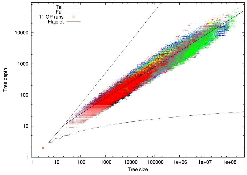
Figure 11: Plot of size and depth of the best individual in each generation for six Sextic polynomial runs
with population of 500. Binary trees must lie between short fat trees (lower curvep“Full”) and “Tall” stringy
trees. Most trees are randomly shaped and lie near the Flajolet limit (depth ≈ 2π|size|, solid line, note
log-log scales).
12Figure 12: Fitness convergence in first Sextic polynomial pop=500 run. In 30% of this run, the whole
population has identical fitness (y=0). Mean prog size (linear scale, black) and best fitness (log, blue)
plotted in the background.
4.3 Results Population 48 trees
In the final experiments the population was reduced still further to allow still larger trees to be evolved.
Whereas in the Boolean experiments Langdon (2017) we reduced the population to 50, this was before we
had access to servers with 48 cores. Therefore these smallest population runs were run with a population
of 48, since this should readily map well to the available Intel mult-core servers.
With the small population, none of the runs solve the problems. Indeed only three runs got close on 40
or more test cases (see Figure 13 and Table 4). Of the remaining eight, only one finds a large number of
fitness improvements. Seven runs contain only between 3 and 30 generations containing fitness improve-
ment, column 3 in Table 4. In three of these, the population gets trapped at trees with just three nodes
which evaluate to constants 0.0626506, 0.069169 and 0.0830508. Although eventually the population does
eventually escape and large trees evolve by the end of the run. Except for these three runs, all the other runs
contain populations where every member of the population has identical fitness. Therefore their maximum
convergence is 48 (see last column in Table 4).
As expected, as with larger populations, the evolved highly binary trees are again approximately the same
shape as random trees. See Figure 15.
Figure 16 shows for almost the whole run the best fitness in the population is fixed but once trees get
big enough further size changes are essentially random. Notice fitness depends only on the sum of the
absolute difference between the value returned by the GP tree and the target value. In particular the “hits”
is only used for reporting. The best fitness found in this run is given by robust trees which always return
a midpoint value (cf. Figure 4) which only passes close to four test points. Trees which closely matched
more test points were discovered in the first nineteen generation of this run. However, in terms of fitness,
they scored worse than a constant and so went extinct.
130.1
13 13 10 13 34 3 8
Best fitness = Mean |error| 48 fixed test cases
1707
0.01
452
2966
814
1 10 100 1000 10000 100000 1e+06
Generation
Figure 13: Evolution of mean absolute error in 11 runs of Sextic polynomial Koza (1992) with population
of 48. (Up to a million generation or aborted on running out of memory, 500 million node limit.) End of
run label gives number of generations when fitness got better. (Seven shown at top right to avoid crowding.)
Table 4: 11 Sextic polynomial runs with population of 48
Gens smallest error impr7 hits size106 power law conv
1000000 0.046215700 11 16 63.920 1.633 48
491618 0.002748230 745 46 396.576 2.060 48
1000000 0.046215700 7 13 190.654 1.448 48
689414 0.004857990 448 40 159.949 1.260 48
1000000 0.046215700 8 14 50.365 1.701 48
143251 0.046215700 11 14 99.541 1.672 48
212528 0.046650600 30 14 257.766 na 42
1000000 0.046730800 3 14 0.000 na 42
958147 0.023259300 1683 18 308.958 1.791 48
294098 0.047174400 3 12 308.121 na 43
757830 0.002985980 2921 44 294.821 1.320 48
7 Figure 13 gives number of generations which improve on their parents, whereas here we give strictly
better than anything previously evolved. Hence slight differences.
14Figure 14: Evolution of tree size in first Sextic run with a population of 48. This run ran for a million gen-
erations. Straight line shows best RMS error power law fit between generation 10 and 1000, y = 0.75x1.63
Figure 15: Plot of size and depth of the best individual in each generation for eleven Sextic polynomial
runs with population of 48.
15Figure 16: Fitness convergence in first Sextic polynomial run with population of 48 trees After generation
19 the best tree in every generation has a fitness of -0.0462157 (4 hits) (tree returns 0.0769947 regardless of
test case, cf. Figure 4). In 90% of this run, the whole population has identical fitness (y=0). (Mean number
of poor fitness children is 0.1315.) Mean prog size (linear scale, black) and best fitness (log, blue).
Figure 17: Fitness convergence in last Sextic polynomial run with population of 48 trees. (Run 295 in
Figure 2.) In this run 67% of generations all 48 trees have identical fitness. The last improvement is found
in generation 752 071 (5759 generation before the end of the run) in a tree of 13 196 331 nodes. It takes over
the whole population in 4 generations. However in 21% of the remaining generations it does not totally
dominate (mean number trees with lower fitness 0.394 per generation). Mean prog size (linear scale, black)
and best fitness (log, blue).
165 Is there a Limit to Evolution?
In the Sextic Polynomial experiments with larger populations there is no hint of either evolution of fitness
or bloat totally stopping. In the smaller populations, it is both possible to run evolution for longer and to
allow trees to bloat to be even larger. Four of the eleven extended runs reached a million generations but in
the remaining seven, bloat ran into memory limits and halted the run. Only in one run did we see anti-bloat,
in which the population converged in a few generation on a small high fitness tree which crossover was
able to replicate across a million generations. Interestingly two other runs found similar solution but after
thousands of generations crossover found bloated version of them.
In the binary 6-Mux Boolean problem Langdon (2017) there are only 65 different fitness values. Therefore
the number of fitness improvements is very limited. An end to bloat was found. By which we mean it was
possible for trees to grow so large that crossover was unable to disrupt the important part of their calculation
next to the root node and many generations were evolved where everyone had identical fitness. This lead
to random selection and random fluctuations in tree size. (I.e. enormous trees but without a tendency for
progressive end less growth.)
This did not happen here. Even in some of the smallest Sextic polynomials runs, we are still seeing
innovation in the second half of the run, with tiny fitness improvements being created by crossover between
enormous parents. Also we are still slightly short of total fitness convergence. Even with populations
containing Sextic polynomial trees of hundreds of millions of nodes, crossover can still be disruptive and
frequently even tiny populations can contain a tree of lower fitness. This is sufficient to provide some
pressure (over thousands of generations) for tree size to increase on average.
Can bloat continue forever? It is still difficult to be definitive in our answer. We have seen cases where
it does not and of course there are plenty of engineering techniques to prevent bloat. But we see other
cases where crossover over thousands of generations can create an innovative child which allows bloat
into a converged population of small tress. Perhaps more interestingly, we see crossover finding fitness
improvement in bloated trees after many thousand of generations.
It is still an open question in continuous domains if, given sufficient memory and computational resources,
bloat will always stifle innovation so completely that crossover will always only reproduce children of
exactly the same fitness for long enough that the lack of selection pressure Langdon and Poli (1997) will
in turn stifle bloat.
6 Conclusions
The availability of mult-core SIMD capable hardware has allowed us to push GP performance on single
computers with floating point problems to that previously only approached with sub-machine code GP
operating in discreet domains Poli and Langdon (1999); Poli and Page (2000). This in turn has allowed GP
runs far longer than anything previously attempted whilst evolving far bigger programs.
As expected, without size or depth limits or biases crossover with brutal selection pressure tends to evolve
very large non-parsimonious programs. Known in the GP community as bloat (page 2 (Koza, 1992,
page 617)). After a few initial generations, GP tree bloat typically follows a sub-quadratic power law Lang-
don (2000a). But eventually effective selection pressure (Nordin, 1997, sec. 14.2), (Banzhaf et al., 1998,
page 187), Stephens and Waelbroeck (1999), Langdon and Poli (2002) within highly evolved populations
falls, leading to bloat at a reduced rate. However we only see the chaotic lack of bloat found in long
running Boolean problems Langdon (2017) in a few unsuccessful runs with tiny populations (red plots in
Figure 2, page 3). Nevertheless in all cases bloated binary trees evolve to be randomly shaped and lie close
to Flajolet’s square root limit (Section 2.2).
Evolving binary Sextic polynomial trees for up to a million generations, during which some programs grow
to four hundred million nodes, suggests even a simple floating point benchmark allows long term fitness
improvement over thousands of generations.
17Acknowledgements
This work was inspired by conversations at Dagstuhl Seminar 18052 on Genetic Improvement of Software.
The new parallel GPQuick code is available via http://www.cs.ucl.ac.uk/staff/W.Langdon/
ftp/gp-code/GPavx.tar.gz
References
Altenberg, L. (1994). The evolution of evolvability in genetic programming. In Kinnear, Jr., K. E., editor, Advances in Genetic
Programming, chapter 3, pages 47–74. MIT Press.
Angeline, P. J. (1994). Genetic programming and emergent intelligence. In Kinnear, Jr., K. E., editor, Advances in Genetic
Programming, chapter 4, pages 75–98. MIT Press.
Banzhaf, W., Nordin, P., Keller, R. E., and Francone, F. D. (1998). Genetic Programming – An Introduction; On the Automatic
Evolution of Computer Programs and its Applications. Morgan Kaufmann, San Francisco, CA, USA.
Keith, M. J. and Martin, M. C. (1994). Genetic programming in C++: Implementation issues. In Kinnear, Jr., K. E., editor,
Advances in Genetic Programming, chapter 13, pages 285–310. MIT Press.
Koza, J. R. (1992). Genetic Programming: On the Programming of Computers by Means of Natural Selection. MIT Press,
Cambridge, MA, USA.
Koza, J. R. (1994). Genetic Programming II: Automatic Discovery of Reusable Programs. MIT Press, Cambridge Massachusetts.
Langdon, W. B. (1998). Genetic Programming and Data Structures: Genetic Programming + Data Structures = Automatic
Programming!, volume 1 of Genetic Programming. Kluwer, Boston.
Langdon, W. B. (1999a). Linear increase in tree height leads to sub-quadratic bloat. In Haynes, T. et al., editors, Foundations of
Genetic Programming, pages 55–56, Orlando, Florida, USA.
Langdon, W. B. (1999b). Scaling of program tree fitness spaces. Evolutionary Computation, 7(4):399–428.
Langdon, W. B. (1999c). Size fair and homologous tree genetic programming crossovers. In Banzhaf, W. et al., editors, Proceed-
ings of the Genetic and Evolutionary Computation Conference, volume 2, pages 1092–1097, Orlando, Florida, USA. Morgan
Kaufmann.
Langdon, W. B. (2000a). Quadratic bloat in genetic programming. In Whitley, D. et al., editors, Proceedings of the Genetic and
Evolutionary Computation Conference (GECCO-2000), pages 451–458, Las Vegas, Nevada, USA. Morgan Kaufmann.
Langdon, W. B. (2000b). Size fair and homologous tree genetic programming crossovers. Genetic Programming and Evolvable
Machines, 1(1/2):95–119.
Langdon, W. B. (2013). Large scale bioinformatics data mining with parallel genetic programming on graphics processing units.
In Tsutsui, S. and Collet, P., editors, Massively Parallel Evolutionary Computation on GPGPUs, Natural Computing Series,
chapter 15, pages 311–347. Springer.
Langdon, W. B. (2017). Long-term evolution of genetic programming populations. In GECCO 2017: The Genetic and Evolution-
ary Computation Conference, pages 235–236, Berlin. ACM.
Langdon, W. B. and Poli, R. (1997). Fitness causes bloat. In Chawdhry, P. K. et al., editors, Soft Computing in Engineering Design
and Manufacturing, pages 13–22. Springer-Verlag London.
Langdon, W. B. and Poli, R. (2002). Foundations of Genetic Programming. Springer-Verlag.
Langdon, W. B., Soule, T., Poli, R., and Foster, J. A. (1999). The evolution of size and shape. In Spector, L. et al., editors,
Advances in Genetic Programming 3, chapter 8, pages 163–190. MIT Press, Cambridge, MA, USA.
Lenski, R. E. et al. (2015). Sustained fitness gains and variability in fitness trajectories in the long-term evolution experiment with
Escherichia coli. Proceedings of the Royal Society B, 282(1821).
McPhee, N. F. and Poli, R. (2001). A schema theory analysis of the evolution of size in genetic programming with linear
representations. In Miller, J. F. et al., editors, Genetic Programming, Proceedings of EuroGP’2001, volume 2038 of LNCS,
pages 108–125, Lake Como, Italy. Springer-Verlag.
Nordin, P. (1997). Evolutionary Program Induction of Binary Machine Code and its Applications. PhD thesis, der Universitat
Dortmund am Fachereich Informatik.
18Poli, R. and Langdon, W. B. (1999). Sub-machine-code genetic programming. In Spector, L. et al., editors, Advances in Genetic
Programming 3, chapter 13, pages 301–323. MIT Press, Cambridge, MA, USA.
Poli, R., Langdon, W. B., and McPhee, N. F. (2008). A field guide to genetic programming. Published via http://lulu.com
and freely available at http://www.gp-field-guide.org.uk. (With contributions by J. R. Koza).
Poli, R. and Page, J. (2000). Solving high-order Boolean parity problems with smooth uniform crossover, sub-machine code GP
and demes. Genetic Programming and Evolvable Machines, 1(1/2):37–56.
Sedgewick, R. and Flajolet, P. (1996). An Introduction to the Analysis of Algorithms. Addison-Wesley.
Singleton, A. (1994). Genetic programming with C++. BYTE, pages 171–176.
Stephens, C. and Waelbroeck, H. (1999). Schemata evolution and building blocks. Evolutionary Computation, 7(2):109–124.
Syswerda, G. (1990). A study of reproduction in generational and steady state genetic algorithms. In Rawlings, G. J. E., editor,
Foundations of genetic algorithms, pages 94–101. Morgan Kaufmann, Indiana University. Published 1991.
Tackett, W. A. (1994). Recombination, Selection, and the Genetic Construction of Computer Programs. PhD thesis, University of
Southern California, Department of Electrical Engineering Systems, USA.
19You can also read