Integraal plan Boven-Zeeschelde - 13_131_18 FHR reports Sub report 18 Effect of the C-alternatives on mud transport www.fl ...
←
→
Page content transcription
If your browser does not render page correctly, please read the page content below
13_131_18
 FHR reports

Integraal plan Boven-Zeeschelde

 Sub report 18
Effect of the C-alternatives on mud transport

 www.flandershydraulicsresearch.be
Integraal Plan Bovenzeeschelde

Sub report 18 – Effect of the C-alternatives on mud transport

 Bi, Q.; Vanlede, J.; Smolders, S.; Mostaert, F.
Cover figure © The Government of Flanders, Department of Mobility and Public Works, Flanders Hydraulics Research Legal notice Flanders Hydraulics Research is of the opinion that the information and positions in this report are substantiated by the available data and knowledge at the time of writing. The positions taken in this report are those of Flanders Hydraulics Research and do not reflect necessarily the opinion of the Government of Flanders or any of its institutions. Flanders Hydraulics Research nor any person or company acting on behalf of Flanders Hydraulics Research is responsible for any loss or damage arising from the use of the information in this report. Copyright and citation © The Government of Flanders, Department of Mobility and Public Works, Flanders Hydraulics Research 2021 D/2021/3241/141 This publication should be cited as follows: Bi, Q.; Vanlede, J.; Smolders, S.; Mostaert, F. (2021). Integraal Plan Bovenzeeschelde: Sub report 18 – Effect of the C- alternatives on mud transport. Version 3.0. FHR Reports, 13_131_18. Flanders Hydraulics Research: Antwerp Reproduction of and reference to this publication is authorised provided the source is acknowledged correctly. Document identification Customer: IMDC iov. dVW-RegioCentraal Ref.: WL2021R13_131_18 Keywords (3-5): Scaldis; mud; sediment transport Knowledge domains: Hydraulics and sediment > Sediment > Cohesive sediment > Numerical modelling Text (p.): 58 Appendices (p.): 9 Confidential: ܈No ܈Available online Author(s): Bi, Q. Control Name Signature Getekend door:Joris Vanlede (Signature) Getekend door:Sven Smolders (Signature Getekend op:2021-07-12 15:52:10 +02:0 Getekend op:2021-07-12 15:47:33 +02:0 Reden:Ik keur dit document goed Reden:Ik keur dit document goed Reviser(s): Vanlede, J., Smolders, S. Getekend door:Joris Vanlede (Signature) Getekend op:2021-07-12 15:54:02 +02:0 Reden:Ik keur dit document goed Project leader: Vanlede, J. Approval Getekend door:Stefan Geerts (Signature) Getekend op:2021-07-13 08:49:22 +02:0 Reden:Ik keur dit document goed Head of Division: Mostaert, F. F-WL-PP10-2 Version 7 Valid as from 3/01/2017
Integraal Plan Bovenzeeschelde - Sub report 18 – Effect of the C-alternatives on mud transport

Abstract

The calibrated mud transport model based on the 3D Scaldis HD model is used to analyse the effects of three
potential alternative bathymetries: the C alternatives. This report describes the effects of the C alternatives
against a future reference situation (2050REF_C). The focus is on the effects on the mud transport and
suspended sediment concentrations in the Upper Sea Scheldt, under 3 different scenarios (boundary
conditions), namely A0CN, AminCL and AplusCH.
The model results are described in terms of differences between the reference run and the C alternatives.
They are presented and interpreted in multiple ways as (1) the relative effect on suspended sediment
concentration (ΔSSC), (2) the decomposed sediment transport (advection and tidal pumping), and (3) plots
of expected sedimentation and erosion. The results are synthesised in a discussion for each alternative.

 Final version WL2021R13_131_18 III

F-WL-PP10-2 Version 7
Valid as from 3/01/2017
Integraal Plan Bovenzeeschelde - Sub report 18 – Effect of the C-alternatives on mud transport

Contents

Abstract ............................................................................................................................................................ III
Contents ............................................................................................................................................................ V
List of tables..................................................................................................................................................... VII
List of figures .................................................................................................................................................. VIII
1 Introduction ............................................................................................................................................... 1
2 Units and reference plane ......................................................................................................................... 2
3 The Calibrated Mud Model and Scenarios ................................................................................................ 3
 3.1 Model set-up ..................................................................................................................................... 3
 3.1.1 Parametrisation of dredging and disposal................................................................................. 3
 3.1.2 Roughness parametrisation....................................................................................................... 4
 3.1.3 The reference bathymetry and the bathymetry of C-alternatives ............................................ 4
 3.2 Boundary conditions........................................................................................................................ 15
 3.2.1 Upstream Boundary Conditions .............................................................................................. 15
 3.2.2 Downstream Boundary Conditions ......................................................................................... 15
 3.3 Initialization of the model ............................................................................................................... 16
 3.4 Alternatives and scenarios for the mud model ............................................................................... 16
 3.4.1 Representative discharges for 2013 and 2050 ........................................................................ 16
 3.4.2 Tidal range scenarios ............................................................................................................... 17
 3.4.3 Sea level rise scenarios ............................................................................................................ 18
 3.4.4 Scenarios for the mud model .................................................................................................. 18
 3.4.5 Overview of Model Runs ......................................................................................................... 18
 3.4.6 Simulation period .................................................................................................................... 19
4 Methodology of Determining the Effects ................................................................................................ 20
 4.1 Evaluation Framework..................................................................................................................... 20
 4.2 Polygons and transects .................................................................................................................... 21
 4.3 Tidal Asymmetry .............................................................................................................................. 24
 4.4 Delta SSC (ΔSSC) .............................................................................................................................. 24
 4.5 Decomposition of sediment transport and flux .............................................................................. 25
 4.6 Sedimentation and erosion ............................................................................................................. 27
 4.7 Bed shear stress and its exceedance time....................................................................................... 27
5 Results ..................................................................................................................................................... 29

 Final version WL2021R13_131_18 V
Integraal Plan Bovenzeeschelde - Sub report 18 – Effect of the C-alternatives on mud transport

 5.1 2050C1 ............................................................................................................................................. 29
 5.1.1 SSC and ΔSSC ........................................................................................................................... 29
 5.1.2 Sedimentation plots ................................................................................................................ 34
 5.2 2050C2 ............................................................................................................................................. 36
 5.2.1 SSC and ΔSSC ........................................................................................................................... 36
 5.2.2 Sedimentation plots ................................................................................................................ 40
 5.2.3 Explanatory parameters: bed shear stress and velocity magnitude ....................................... 42
 5.3 2050C3 ............................................................................................................................................. 43
 5.3.1 SSC and ΔSSC ........................................................................................................................... 43
 5.3.2 Sedimentation plots ................................................................................................................ 46
 5.3.3 Explanatory parameter: velocity magnitude ........................................................................... 48
 5.4 Long term sinks................................................................................................................................ 49
 5.4.1 FCA-CRT ................................................................................................................................... 49
 5.4.2 Depoldered areas .................................................................................................................... 50
 5.4.3 Total Sediment Balance ........................................................................................................... 52
6 Discussion and conclusion ....................................................................................................................... 53
 6.1 Discussion ........................................................................................................................................ 53
 6.2 Conclusions ...................................................................................................................................... 56
7 References ............................................................................................................................................... 57
Appendix 1 Polygons for ΔSSC calculation.................................................................................................. A1
 Polygons for 2050C1 .................................................................................................................................... A1
 Polygons for 2050C2 .................................................................................................................................... A3
 Polygons for 2050C3 .................................................................................................................................... A5
Appendix 2 Bottom evolution in FCA-CRTs and depoldering areas over 50 years ..................................... A7

 VI WL2021R13_131_18 Final version
Integraal Plan Bovenzeeschelde - Sub report 18 – Effect of the C-alternatives on mud transport

List of tables

Table 1 – Physical parameters used in the mud model..................................................................................... 3
Table 2 – Overview of all measures in the C alternatives (IMDC, 2021) ........................................................... 5
Table 3 – Imposed mud concentrations at upstream tributaries.................................................................... 15
Table 4 – Tidal range scenarios ....................................................................................................................... 17
Table 5 – List of the different scenarios/alternatives runs.............................................................................. 19
Table 6 – Selected explanatory and evaluation parameters from the evaluation framework ....................... 20

 Final version WL2021R13_131_18 VII
Integraal Plan Bovenzeeschelde - Sub report 18 – Effect of the C-alternatives on mud transport

List of figures

Figure 1 – The bathymetry used in the 2050REF_C .......................................................................................... 4
Figure 2 – Bathymetry of the Upper Sea Scheldt in 2050REF_C (km 1-13) ....................................................... 7
Figure 3 – Bathymetry of the Upper Sea Scheldt in 2050REF_C (km 14-34) ..................................................... 7
Figure 4 – Bathymetry of the Upper Sea Scheldt in 2050REF_C (km 35-56) ..................................................... 8
Figure 5 – Bathymetry of the Upper Sea Scheldt in 2050REF_C (km 56-64) ..................................................... 8
Figure 6 – Bathymetry of the Upper Sea Scheldt in 2050C1 (km 1-13)............................................................. 9
Figure 7 – Bathymetry of the Upper Sea Scheldt in 2050C1 (km 14-34)........................................................... 9
Figure 8 – Bathymetry of the Upper Sea Scheldt in 2050C1 (km 35-56)......................................................... 10
Figure 9 – Bathymetry of the Upper Sea Scheldt in 2050C1 (km 56-64)......................................................... 10
Figure 10 – Bathymetry of the Upper Sea Scheldt in 2050C2 (km 1-13)......................................................... 11
Figure 11 – Bathymetry of the Upper Sea Scheldt in 2050C2 (km 14-34)....................................................... 11
Figure 12 – Bathymetry of the Upper Sea Scheldt in 2050C2 (km 35-56)....................................................... 12
Figure 13 – Bathymetry of the Upper Sea Scheldt in 2050C2 (km 56-64)....................................................... 12
Figure 14 – Bathymetry of the Upper Sea Scheldt in 2050C3 (km 1-13)......................................................... 13
Figure 15 – Bathymetry of the Upper Sea Scheldt in 2050C3 (km 14-34)....................................................... 13
Figure 16 – Bathymetry of the Upper Sea Scheldt in 2050C3 (km 35-56)....................................................... 14
Figure 17 – Bathymetry of the Upper Sea Scheldt in 2050C3 (km 56-64)....................................................... 14
Figure 18 – Upstream discharges used in mud model scenarios .................................................................... 17
Figure 19 – The zone with changed bottom friction in the tidal range scenarios........................................... 18
Figure 20 – Polygons for 2050_REF_C (polygons 1-13, 87-88) ........................................................................ 21
Figure 21 – Polygons for 2050_REF_C (polygons 13-31, 85-86) ...................................................................... 22
Figure 22 – Polygons for 2050_REF_C (polygons 32-58, 78-84) ...................................................................... 22
Figure 23 – Polygons for 2050_REF_C (polygons 59-77) ................................................................................. 23
Figure 24 – Map of the Scheldt estuary with main tributaries and most important locations. The thalweg is
indicated with the red dotted line................................................................................................................... 23
Figure 25 – Methodology of working with Deltas ........................................................................................... 24
Figure 26 – Bathymetry differences between 2050C1 and 2050REF_C in the Upper Sea Scheldt ................. 29
Figure 27 – Time-averaged surface SSC and depth-average SSC in 2050C1 ................................................... 30
Figure 28 – Depth-averaged sediment concentration in the upstream zone km 0-5 at a certain time step.. 31
Figure 29 – Time-averaged depth-averaged ΔSSC (2050C1) ........................................................................... 31
Figure 30 – Cross-sectionally averaged velocity bias during ebb and flood (2050C1). ................................... 32
Figure 31 – The effect of C1 on the exceedance rate of bed shear stress > 1 Pa in the Upper Sea Scheldt from
km 23-65 (A0CN) ............................................................................................................................................. 33

 VIII WL2021R13_131_18 Final version
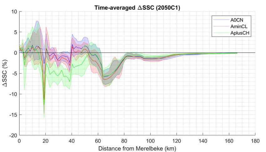
Integraal Plan Bovenzeeschelde - Sub report 18 – Effect of the C-alternatives on mud transport

Figure 32 – Comparison of depth-averaged and surface ΔSSC (2050C1_A0CN)............................................. 33
Figure 33 – Time-averaged vertical profiles of SSC at km 19 in the main channel in 2050REF_C_A0CN and
2050C1_A0CN .................................................................................................................................................. 34
Figure 34 – Effect of C1 on sedimentation and erosion (m) after 40 days from Km24-65 (A0CN) ................. 35
Figure 35 – Effect of C1 on sedimentation and erosion after 40 days from Km1-23 (A0CN) ......................... 35
Figure 36 – Time-averaged surface SSC and depth-average SSC in 2050C2 ................................................... 37
Figure 37 – Bathymetry differences between 2050C2 and 2050REF_C in the Upper Sea Scheldt ................. 38
Figure 38 – Time-averaged depth-averaged ΔSSC (2050C2) ........................................................................... 38
Figure 39 – Effect of 2050C2 on tidal asymmetry Tflood/Tebb............................................................................ 39
Figure 40 – Comparison of depth-averaged and surface ΔSSC (2050C2_A0CN)............................................. 40
Figure 41 – Effect of C2 on sedimentation and erosion (m) after 40 days from Km24-65 (A0CN) ................. 41
Figure 42 – Effect of C2 on sedimentation and erosion (m) after 40 days from Km1-23 (A0CN) ................... 41
Figure 43 – The effect of C2 on the exceedance rate of bed shear stress > 1 Pa in the Upper Sea Scheldt from
km 23-65 (A0CN) ............................................................................................................................................. 42
Figure 44 – The effect of C2 on the frequency of velocity magnitude > 0.65 m/s in the Upper Sea Scheldt from
km 1-23 (A0CN) ............................................................................................................................................... 42
Figure 45 – Time-averaged surface SSC and depth-average SSC in 2050C3 ................................................... 43
Figure 46 – Bathymetry differences between 2050C3 and 2050REF_C in the Upper Sea Scheldt ................. 44
Figure 47 – Time-averaged depth-averaged ΔSSC (2050C3) ........................................................................... 45
Figure 48 – Comparison of depth-averaged and surface ΔSSC (2050C3_A0CN)............................................. 46
Figure 49 – Effect of C3 on sedimentation and erosion (m) after 40 days from Km24-65 (A0CN) ................. 47
Figure 50 – Effect of C3 on sedimentation and erosion (m) after 40 days from Km1-23 (A0CN) ................... 47
Figure 51 – The effect of C3 on the frequency of velocity magnitude > 0.65 m/s in the Upper Sea Scheldt from
km 1-23 (A0CN) ............................................................................................................................................... 48
Figure 52 – Sedimentation rate in FCA-CRTs expressed in TDM/yr ................................................................ 49
Figure 53 – Sedimentation rate expressed in TDM/yr in depoldered areas (2050REF_C).............................. 50
Figure 54 – Sedimentation rate expressed in TDM/yr in depoldered areas (2050C1).................................... 50
Figure 55 – Sedimentation rate expressed in TDM/yr in depoldered areas (2050C2).................................... 51
Figure 56 – Sedimentation rate expressed in TDM/yr in depoldered areas (2050C3).................................... 51
Figure 57 – The estimated yearly sedimentation averaged over 50 years ..................................................... 52
Figure 58 – Time-averaged depth-averaged SSC along the Scheldt estuary (A0CN) ...................................... 53
Figure 59 – The time-averaged depth-averaged ΔSSC of C alternatives (A0CN) ............................................ 54
Figure 60 – Averaged total sediment transport (A0CN) .................................................................................. 55
Figure 61 – Averaged sediment transport due to advection (A0CN) .............................................................. 55
Figure 62 – Averaged sediment transport due to tidal pumping (A0CN)........................................................ 56
Figure 63 – Polygons for 2050_C1 (polygons 1-13, 87-88) .............................................................................. A1
Figure 64 – Polygons for 2050_C1 (polygons 13-31, 85-86) ............................................................................ A1

 Final version WL2021R13_131_18 IX
Integraal Plan Bovenzeeschelde - Sub report 18 – Effect of the C-alternatives on mud transport

Figure 65 – Polygons for 2050_C1 (polygons 32-58, 79-84) ............................................................................ A2
Figure 66 – Polygons for 2050_C1 (polygons 59-78) ....................................................................................... A2
Figure 67 – Polygons for 2050_C2 (polygons 1-13, 91-92) .............................................................................. A3
Figure 68 – Polygons for 2050_C2 (polygons 13-31, 89-90) ............................................................................ A3
Figure 69 – Polygons for 2050_C2 (polygons 32-58, 79-88) ............................................................................ A4
Figure 70 – Polygons for 2050_C2 (polygons 59-78) ....................................................................................... A4
Figure 71 – Polygons for 2050_C3 (polygons 1-13, 90-91) .............................................................................. A5
Figure 72 – Polygons for 2050_C3 (polygons 13-31, 88-89) ............................................................................ A5
Figure 73 – Polygons for 2050_C3 (polygons 32-58, 79-87) ............................................................................ A6
Figure 74 – Polygons for 2050_C3 (polygons 59-78) ....................................................................................... A6
Figure 75 – Sedimentation rate in FCA-CRTs over 50 years ............................................................................ A7
Figure 76 – Sedimentation rate in depoldered areas with sea level rise (2050REF_C)................................... A8
Figure 77 – Sedimentation rate in depoldered areas with sea level rise (2050C1) ........................................ A8
Figure 78 – Sedimentation rate in depoldered areas with sea level rise (2050C2) ........................................ A9
Figure 79 – Sedimentation rate in depoldered areas with sea level rise (2050C3) ........................................ A9

 X WL2021R13_131_18 Final version
Integraal Plan Bovenzeeschelde - Sub report 18 – Effect of the C-alternatives on mud transport

1 Introduction

Based on the SCALDIS model, a mud transport model, as a part of a high-resolution sediment transport model
for the whole Scheldt estuary is developed and calibrated. The details of the mud model are reported in
Smolders et al. (2018).
The main objective of this mud transport model is to study future (time horizon = 2050)
scenarios/alternatives of the Scheldt estuary by quantifying the effects compared to the reference case, e.g.
the effects on suspended sediment concentration (SSC), sediment flux through zones of interest and
erosion/deposition on intertidal flats and subtidal channels.
The present report describes the model results with new future bathymetry alternatives in the tidal-
influenced zones of the estuary. These new alternatives are called C-alternatives and developed with the
following mindset (IMDC, 2021):
 • C1 alternative: Tackle the most prominent nautical bottlenecks (Km 0 – Ringvaart, km 10 – Wetteren,
 km 15 till km 17 – Hoogland and Uitbergen, Km 30 – Kasteeltje, km 40 – Kramp). Looking for
 opportunities in the river and redefining the Sigma plan to improve habitat and to reduce the
 increase in tidal amplitude.
 • C2 alternative: Tackle also less prominent nautical bottlenecks and define additional measures for
 the most prominent bottlenecks. Include additional opportunities in the valley (depolderings, side
 channels) to improve habitat and to reduce the increase in tidal amplitude.
 • C3 alternative: Yet additional nautical measures for a limited number of locations (Uitbergen,
 Paardenweide, Kasteeltje) and additional measures (larger depolderings, additional depoldering at
 Weert, undeepening at Temse) aiming at providing extra system resilience while also improving
 habitat conditions.
All the C alternatives are designed based on the sustainable bathymetry for 2050 (IMDC, 2015). The overview
of the implemented measures is described in Bi et al. (2020a).

 Final version WL2021R13_131_18 1
Integraal Plan Bovenzeeschelde - Sub report 18 – Effect of the C-alternatives on mud transport

2 Units and reference plane

Time is expressed in CET (Central European Time).
Depth, height and water levels are expressed in meter TAW (Tweede Algemene Waterpassing).
Bathymetry and water levels are positive above the reference plane.
The horizontal coordinate system is RD Parijs.
Distance along the estuary is measured in km from the lock in Merelbeke.

 2 WL2021R13_131_18 Final version
Integraal Plan Bovenzeeschelde - Sub report 18 – Effect of the C-alternatives on mud transport

3 The Calibrated Mud Model and Scenarios

3.1 Model set-up
The mud model used for the analysis of C alternatives is based on the same calibrated mud model used in
the analysis of B alternatives (Bi et al., 2018). The main difference between the mud model for C- and the
B-alternatives is the computational grid or the mesh.
Due to the new measures in C-alternatives (C1-C2-C3), the previous mesh has to be extended to
accommodate the additional depoldered and FCA/FCA-CRT areas. Moreover, the new FCA/FCA-CRT areas
also require updating the configuration of culverts in the domain. The rest of the model settings are kept the
same as in the mud model for the B alternatives. An overview of the physical parameters for the mud model
is given in Table 1.

 Table 1 – Physical parameters used in the mud model

 Physical parameters CAL_007

 INITIAL MUD CONCENTRATION (g/L) 0.5

 DENSITY OF THE SEDIMENT (kg/m3) 2650

 CONSTANT SEDIMENT SETTLING VELOCITY (m/s) 5.0E-04

 HINDERED SETTLING NO

 NUMBER OF SEDIMENT BED LAYERS 1

 INITIAL THICKNESS OF SEDIMENT LAYERS (m) 0.0

 MUD CONCENTRATIONS PER LAYER (kg/m3) 500

 EROSION COEFFICIENT (kg/m2/s) 1.0E-04

 CRITICAL EROSION SHEAR STRESS OF THE MUD LAYERS (Pa) 0.05

 CRITICAL SHEAR STRESS FOR DEPOSITION (Pa) 1.0E06

3.1.1 Parametrisation of dredging and disposal
A point source is placed in the model near Oosterweel, releasing disposed material into the water column.
This is used to simulate the sediment disposal process in the 3D sediment transport model. According to the
field observations, the yearly averaged amount of sediment deposited back in the estuary is 4.545.995 Tons
(averaged over period 2007 – 2015). This number is converted into a constant sediment release rate at the
point source to make sure the same amount of material is put back into the system. This point source remains
the same in all the reference cases and the C alternatives.

 Final version WL2021R13_131_18 3
Integraal Plan Bovenzeeschelde - Sub report 18 – Effect of the C-alternatives on mud transport

In the mud model there is no material dredged from the locks and docks. Although the amount of deposition
and erosion is recorded, the bottom elevation is not updated due to decoupling between hydrodynamics and
bottom evolution. Therefore, there is no effect .

3.1.2 Roughness parametrisation
Instead of using spatial varying bottom roughness (Manning coefficients) as in the hydrodynamic model, a
constant and uniform Manning coefficient (0.02) is used in the mud model, same as in the model for the B
alternatives (Smolders et al., 2018). Therefore, only flow velocity and water level are used from the
hydrodynamics in the mud model, while the bed shear stress for erosion-deposition is computed separately.
The reason for using a different roughness coefficient in the mud model is that the spatial variable Manning
coefficients used in the hydrodynamic model are correcting for more than only the differences in bottom
roughness, e.g. a turbulence model that might be too dissipative in the more meandering parts of the estuary.
Using the same roughness of the HD model in the mud model gives undesired patterns in the calculation of
the bottom shear stress and erosion rates.

3.1.3 The reference bathymetry and the bathymetry of C-alternatives
For implementing the three different C alternatives (C1, C2 and C3) in the SCALDIS model, a new reference
grid is created based on the original 2050REF grid used in the B-alternatives (2050REF_B). This new reference
grid, named 2050REF_C, is then used as the basis for implementing the C alternatives.

 Figure 1 – The bathymetry used in the 2050REF_C

The new reference grid is obtained by extending and refining the 2050REF_B mesh in the Upper Sea Scheldt
in order to include the maximum outline of all C alternatives. For the rest of the domain except in the
Ringvaart (a widened and deepened Ringvaart is applied to the 2050REF_C and the C alternatives), the grid
remains unmodified, in order to allow the reuse of the boundary data. In the extended areas in the Upper
Sea Scheldt, the finest grid resolution is about 7 m, and the coarsest resolution is about 50 m.
The new reference grid is able to accommodate the adaptations of the navigation channel, the new
development of intertidal nature and the additional de-embankments and FCAs (with and without CRT),
which are considered in any of the C alternatives.

 4 WL2021R13_131_18 Final version
Integraal Plan Bovenzeeschelde - Sub report 18 – Effect of the C-alternatives on mud transport

The sustainable bathymetry in the 2050REF_B grid is adapted by deepening and widening of the Ringvaart
and becomes the new reference grid 2050REF_C. For the extended areas in 2050REF_C, the background
bathymetry that represents the current situation (provided by IMDC) is mapped to the mesh.
When incorporating the C alternatives, the new bathymetry from C1, C2 and C3 is mapped to the 2050REF_C
grid, respectively. The overview of the implemented measures in the C alternatives is presented in Table 2.

 Table 2 – Overview of all measures in the C alternatives (IMDC, 2021)

 Distance to Overview measures MHW MLW
 Merelbeke
 [m [m
 [km] C1 C2 C3
 TAW] TAW]

 Ringvaart 0-3 Deepening and widening (also present in 2050REF_C) 5.05 2.44

 Veerhoek 4.5 - Widening + pull back of dyke 5.05 2.44

 Limited tidal
 Melleham 5.5 CRT without FCA Depoldering 5.05 2.44
 interaction

 Bommels 6.5 - Widening + pull back of dyke 5.06 2.37

 Voorde 9 Bend modifications + intertidal nature 5.07 2.28

 Improved navigation (cfr VaG) by
 Wetteren 11 - 5.08 2.23
 installing sheet piles

 DS Wetteren 12.5 Depoldering 5.08 2.23

 FCA Wijmeers 15 - Additional FCA in the north 5.08 2.12

 Wijmeers Bend cut off (C1: variant 1, C2: variant 2, C3: variant 3) +
 16 5.10 2.10
 (Hoogland) intertidal nature+FCA
 Bend cut off + intertidal nature+depoldering
 Uitbergen 19 5.10 2.02
 (C1: variant 1, C2: variant 2, C3: variant 3)
 Paardenweide Bend cut
 21 - - 5.10 1.95
 (Wichelen) off+depoldering
 Depoldering
 Depoldering variant
 Oude Broekmeer 24-27 - variant 1 + side 5.17 1.63
 2 + side channel
 channel
 Appels
 28 Improved navigation by smoothing the bend (cfr Chafing) 5.20 1.50
 (Scheldebroek)

 Scheldebroek 28 FCA Scheldebroek converted into FCA-CRT 5.20 1.50

 Depoldering Depoldering variant
 Sint-Onolfspolder 28-30 - variant 1 + side 1 + side channel 5.20 1.50
 channel variant 1 variant 2
 Bend smoothening + intertidal nature
 Kasteeltje 31 5.27 1.24
 (C1: variant 1, C2: variant 2, C3: variant 3)

 Dender 32.5 - Improved navigation by widening channel 5.3 1.12

 Final version WL2021R13_131_18 5
Integraal Plan Bovenzeeschelde - Sub report 18 – Effect of the C-alternatives on mud transport

 Distance to Overview measures MHW MLW
 Merelbeke
 [m [m
 [km] C1 C2 C3
 TAW] TAW]
 Grembergen broek
 35-38 - Depoldering 5.34 1.02
 – Armenput

 Waterleiding 38 Improved navigation (cfr Chafing) by widening channel 5.38 0.91

 Depoldering Depoldering
 Roggeman 39 - 5.40 0.85
 variant 1 variant 2
 Bend cut off + intertidal nature
 Kockham (Kramp) 40 5.44 0.75
 (C1: variant 1; C2-C3: variant 2)

 Wal-Zwijn 44-48 FCA with CRT FCA with CRT FCA with CRT 5.50 0.59

 Depoldering Depoldering
 Blankaart 49 FCA 5.55 0.40
 variant 1 variant 2
 Depoldering
 Akkershoofd 50 - - together with 5.54 0.38
 Blankaart
 New connection with Durme + partly depoldering Tielrode
 Tielrode Broek 55 5.52 0.31
 Broek

 Weert 51-56 - - Depoldering 5.52 0.31

 Local fill-in +
 Temse to Rupel 57-64 Local fill-in reducing channel 5.46 0.15
 depth

 Schouselbroek 59 - Depoldering + new side channel 5.47 0.19

 Schellandpolder 61 - Depoldering + new side channel 5.47 0.16

 Oudbroekpolder 63 - Depoldering + new side channel 5.45 0.13

The bathymetry of the 2050REF_C and the C alternatives are shown below.

 6 WL2021R13_131_18 Final version
Integraal Plan Bovenzeeschelde - Sub report 18 – Effect of the C-alternatives on mud transport

Reference bathymetry
The bathymetry of the 2050REF_C is shown in Figure 2 - Figure 5. There are no new measures defined in this
reference case. The Ringvaart is deepened and included as a no-deposition zone in order to avoid that the
zone acts as a sediment trap (as was the case in the initial B scenarios).

 Figure 2 – Bathymetry of the Upper Sea Scheldt in 2050REF_C (km 1-13)

 Figure 3 – Bathymetry of the Upper Sea Scheldt in 2050REF_C (km 14-34)

 Final version WL2021R13_131_18 7
Integraal Plan Bovenzeeschelde - Sub report 18 – Effect of the C-alternatives on mud transport

 Figure 4 – Bathymetry of the Upper Sea Scheldt in 2050REF_C (km 35-56)

 Figure 5 – Bathymetry of the Upper Sea Scheldt in 2050REF_C (km 56-64)

 8 WL2021R13_131_18 Final version
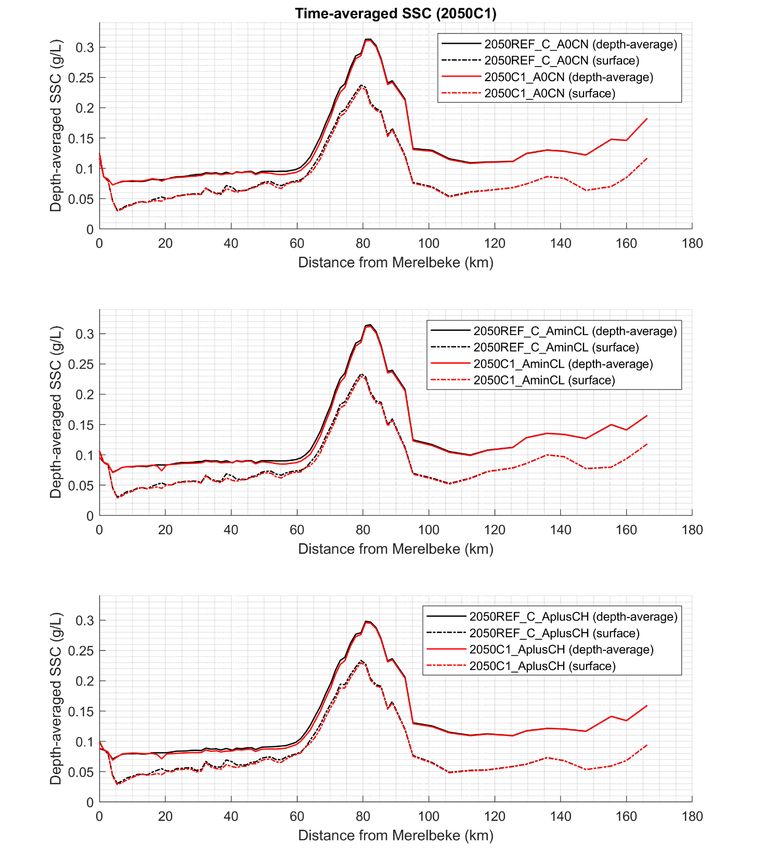
Integraal Plan Bovenzeeschelde - Sub report 18 – Effect of the C-alternatives on mud transport

C1 bathymetry
The bathymetry used of the C1 alternative is shown in Figure 6 - Figure 9. The new measures implemented
in the C1 alternative are listed in Table 2.

 Figure 6 – Bathymetry of the Upper Sea Scheldt in 2050C1 (km 1-13)

 Figure 7 – Bathymetry of the Upper Sea Scheldt in 2050C1 (km 14-34)

 Final version WL2021R13_131_18 9
Integraal Plan Bovenzeeschelde - Sub report 18 – Effect of the C-alternatives on mud transport

 Figure 8 – Bathymetry of the Upper Sea Scheldt in 2050C1 (km 35-56)

 Figure 9 – Bathymetry of the Upper Sea Scheldt in 2050C1 (km 56-64)

 10 WL2021R13_131_18 Final version
Integraal Plan Bovenzeeschelde - Sub report 18 – Effect of the C-alternatives on mud transport

C2 bathymetry
The bathymetry used of the C2 alternative is shown in Figure 10 - Figure 13. The new measures implemented
in the C2 alternative can be seen in Table 2.

 Figure 10 – Bathymetry of the Upper Sea Scheldt in 2050C2 (km 1-13)

 Figure 11 – Bathymetry of the Upper Sea Scheldt in 2050C2 (km 14-34)

 Final version WL2021R13_131_18 11
Integraal Plan Bovenzeeschelde - Sub report 18 – Effect of the C-alternatives on mud transport

 Figure 12 – Bathymetry of the Upper Sea Scheldt in 2050C2 (km 35-56)

 Figure 13 – Bathymetry of the Upper Sea Scheldt in 2050C2 (km 56-64)

 12 WL2021R13_131_18 Final version
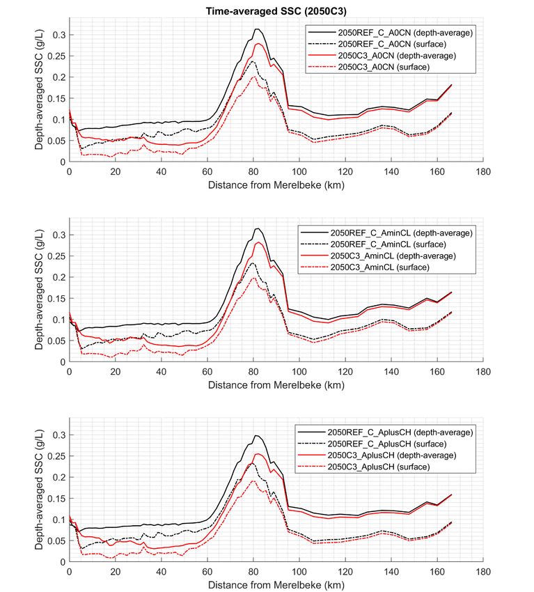
Integraal Plan Bovenzeeschelde - Sub report 18 – Effect of the C-alternatives on mud transport

C3 bathymetry
The bathymetry used of the C3 alternative is shown in Figure 14 - Figure 17. The C3 alternative has the most
new measures implemented, as listed in Table 2.

 Figure 14 – Bathymetry of the Upper Sea Scheldt in 2050C3 (km 1-13)

 Figure 15 – Bathymetry of the Upper Sea Scheldt in 2050C3 (km 14-34)

 Final version WL2021R13_131_18 13
Integraal Plan Bovenzeeschelde - Sub report 18 – Effect of the C-alternatives on mud transport

 Figure 16 – Bathymetry of the Upper Sea Scheldt in 2050C3 (km 35-56)

 Figure 17 – Bathymetry of the Upper Sea Scheldt in 2050C3 (km 56-64)

 14 WL2021R13_131_18 Final version
Integraal Plan Bovenzeeschelde - Sub report 18 – Effect of the C-alternatives on mud transport

3.2 Boundary conditions

3.2.1 Upstream Boundary Conditions
Upstream tributaries feed the model with a discharge. There are 8 upstream boundaries with prescribed
discharge and suspended sediment concentration. Discharges are defined as upstream boundary conditions
at the Upper Sea Scheldt for Merelbeke, Dender, Zenne, Dijle, Kleine Nete, Grote Nete, Kanaal
Gent - Terneuzen (Smolders et al., 2016). See also section 3.4.1 for the representative discharges.

 Table 3 – Imposed mud concentrations at upstream tributaries

 Imposed concentration
 Tributaries
 (g/L)
 Dender 0.098

 Zenne 0.062

 Kleine Nete 0.041

 Dijle 0.074

 Grote Nete 0.045

 Merelbeke 0.094

Besides of the discharges, in the mud model, sediment concentration is imposed to each upstream
tributaries. The imposed sediment concentration is calculated based on the yearly averaged redistributed
sediment loads as shown in Table 3 (taken from Smolders et al., 2018). These imposed concentrations stay
the same in all the reference cases and scenarios. Because the upstream discharge is synthetic and remains
constant most of the time (with a peak event in a short duration), the imposed SSC is derived based on the
yearly sediment input.

3.2.2 Downstream Boundary Conditions
A model chain is used to generate downstream boundary conditions for the mud model. There are two levels
of nesting involved in this procedure, from CSM (Continental Shelf Model) to ZUNO (Zuidelijke Noordzee),
and from ZUNO to SCALDIS. Sea level rise (SLR) is implemented in the boundary of the CSM model. The effect
of SLR is calculated throughout the model chain.
Both water level and velocities are used as downstream boundary conditions in the SCALDIS mud model. This
resolves instability issues near the North Sea boundary when there was only water level imposed in earlier
versions of SCALDIS.
For the actual situation, the ZUNO model (ZUNO_2013_harmonic) is used for obtaining water levels, velocity
and salinity at the downstream boundary.
For scenarios including Sea Level Rise The downstream boundary conditions in the mud model are inherited
from the CSM-ZUNO model chain, in which the sea level rise is added into the boundary conditions of the
CSM model. To be more specific, the CSM models with sea level rise scenarios
(“CSM_2050_noWind_plus15cm” and “CSM_2050_noWind_plus40cm”) are used. In this case, the nested
ZUNO model will naturally have sea level rise when it uses the water levels generated by CSM models as its

 Final version WL2021R13_131_18 15
Integraal Plan Bovenzeeschelde - Sub report 18 – Effect of the C-alternatives on mud transport

boundary conditions. The mud model is then nested in ZUNO model, and will therefore “inherit” the sea level
rise by using water levels, velocity and salinity from the ZUNO model at its downstream boundary nodes.
The downstream boundary also has a prescribed sediment concentration, which is derived from satellite
images in the study of Fettweis et al. (2007). An average value of 12 mg/L is taken to represent SSC values at
the North Sea. Since the simulation period is relatively short (40 days), seaward boundary is far away from
the zone of interest, it does not significantly affect the Upper Sea Scheldt due to the fact that the Upper Sea
Scheldt is ebb dominant and the net sediment transport is towards downstream, the seaward boundary value
is kept constant over space and time, and remains the same for all alternatives and scenarios described in
this report.

3.3 Initialization of the model
The mud transport model is initialized with an empty bed and uniform suspension concentration of 500 mg/L
as described in Smolders et al. (2018). For the hydrodynamics, the mud model is initialized with the flow field
from the last time step of a 2-day pure-hydrodynamic hotstart run.

3.4 Alternatives and scenarios for the mud model
The calibrated mud transport model is used to evaluate the effects of different C-alternatives (specified
geometry of the Scheldt estuary), under different scenarios (a range of boundary conditions to take into
account climate change, sea level rise, increasing or decreasing tidal amplitude, high or low river discharge).
The list of the scenario runs is presented in Table 5. More information about the SCALDIS model can be found
in (Smolders et al., 2016 ).

3.4.1 Representative discharges for 2013 and 2050
There are two different sets of synthetic discharges used as the upstream boundary conditions in the mud
model scenarios. One is based on the current situations of 2013 (QN2013), and the other one is made for the
future scenarios in 2050 (QN2050). Each of these synthetic time series of discharge contains one event with
a peak discharge.
In Figure 18, the discharges at Melle, Dender and Rupel (the sum of Zenne, Dijle, Grote Nete and Kleine Nete)
for the current situation and for the 2050 scenarios are plotted together. It can be seen that the discharge
becomes larger for Melle and Dender in 2050, and smaller for Rupel. The Rupel basin also has a smaller
average discharge in 2050 compared to the current situation.

 16 WL2021R13_131_18 Final version
Integraal Plan Bovenzeeschelde - Sub report 18 – Effect of the C-alternatives on mud transport

 Figure 18 – Upstream discharges used in mud model scenarios

These two sets of upstream discharges are provided by IMDC, based on statistical analysis for the current
and future scenarios (IMDC, 2015). The discharge for the current situation (QN2013) is applied in the runs
with A0CN scenarios. The discharge for the 2050 (QN2050) is used in the runs with AminCL and AplusCH
scenarios. The list of the runs and their boundaries conditions are summarized in Table 5.

3.4.2 Tidal range scenarios
In this study, tidal range scenarios A+, A0 and A- have been implemented in both the hydrodynamic model
and the mud model. In these three scenarios, the tidal amplitude at Schelle is equal to 5.70, 5.40 and 5.00 m,
respectively (Table 4).

 Table 4 – Tidal range scenarios

 Scenario Bottom friction Tidal amplitude at Schelle (m)

 A+ The bottom friction for hydrodynamics in the 5.70
 Western Scheldt is lowered.

 A0 The bottom friction for hydrodynamics in the 5.40 (current tidal range)
 Western Scheldt remains as in the SCALDIS
 hydrodynamic model.

 A- The bottom friction for hydrodynamics in the 5.00
 Western Scheldt is increased.

 Final version WL2021R13_131_18 17
Integraal Plan Bovenzeeschelde - Sub report 18 – Effect of the C-alternatives on mud transport

The increase and decrease of the tidal range is realised in the model by changing the roughness (Manning
coefficient) in the Western Scheldt. The zone with altered bottom roughness is indicated in Figure 19. For the
scenario “A+”, the Manning coefficient at each point in the red zone is decreased by 0.00426; for the scenario
“A-”, the Manning coefficient at each point in the red zone is increased by 0.00554. These values were
determined by calibration in order to achieve the target tidal amplitudes at Schelle.
For the Western Scheldt, these changes will impact the sediment results in an unrealistic way. However, since
this region is away from the Upper Sea Scheldt, the impact on the model results in the zone of interest is
limited.

 Figure 19 – The zone with changed bottom friction in the tidal range scenarios
 (red indicates the area with changes).

3.4.3 Sea level rise scenarios
The following sea level rise scenarios are modelled in different runs for 2050:
 - The “current” situation (CN, +0 cm in 2050);
 - The “low” scenario (CL, +15 cm in 2050);
 - The “high” scenario (CH, +40 cm in 2050).
The downstream boundary conditions for “CL” and “CH” scenarios are generated from CSM-ZUNO model,
instead of adding the values directly on the water levels at the boundary.

3.4.4 Scenarios for the mud model
The “current” situation CN is always used in the reference cases for comparison, and it is combined with an
unchanged tidal range (A0CN). The tidal range scenario A+ is combined with the sea level rise CH (AplusCH).
The tidal range scenario A- is combined with the sea level rise CL (AminCL). More information about the
scenarios is given in IMDC (2015).

3.4.5 Overview of Model Runs
Twelve model runs are devised to study the effects of C-alternatives on the mud transport. The overview of
model runs is listed in Table 5.

 18 WL2021R13_131_18 Final version
Integraal Plan Bovenzeeschelde - Sub report 18 – Effect of the C-alternatives on mud transport

 Table 5 – List of the different scenarios/alternatives runs

 Bathymetry Discharge Amplitude Sea level
 Code Year
 (alternatives) type correction scenario

 2050REF_C_QN_A0CN QN2013 A0 CN
 2050REF_C_QN_AminCL 2050 REF_C QN2050 A- CL
 2050REF_C_QN_AplusCH QN2050 A+ CH
 2050C1_QN_A0CN QN2013 A0 CN
 2050C1_QN_AminCL 2050 C1 QN2050 A- CL
 2050C1_QN_AplusCH QN2050 A+ CH
 2050C2_QN_A0CN QN2013 A0 CN
 2050C2_QN_AminCL 2050 C2 QN2050 A- CL
 2050C2_QN_AplusCH QN2050 A+ CH
 2050C3_QN_A0CN QN2013 A0 CN
 2050C3_QN_AminCL 2050 C3 QN2050 A- CL
 2050C3_QN_AplusCH QN2050 A+ CH

(A0, A+, A-): Different tidal range scenarios.
(CN, CL, CH): Sea level rise scenarios.

3.4.6 Simulation period
All the runs have a simulation period of 42 days, including a pure hydrodynamic spin up period of 2 days. For
the runs 2050REF_C_QN_A0CN, 2050C1_QN_A0CN, 2050C2_QN_A0CN and 2050C3_QN_A0CN, the
simulation period is from 2013/07/29 22:20:00 to 2013/09/09 22:20:00. For the rest of the runs, the 2050
future scenarios are applied, with the simulation period from 2050/08/09 22:00:00 to 2050/09/20 22:00:00.

 Final version WL2021R13_131_18 19
Integraal Plan Bovenzeeschelde - Sub report 18 – Effect of the C-alternatives on mud transport

4 Methodology of Determining the Effects

4.1 Evaluation Framework
The evaluation of alternatives is based on the evaluation framework for the Integrated Plan Upper Sea
Scheldt. This partial evaluation framework addresses elements of the EIA disciplines Water and Fauna &
Flora. The partial framework is based on the well-established Evaluation Method for the Scheldt Estuary
(EMSE) (IMDC, 2018). The EMSE is a mostly quantitative and multidisciplinary approach to evaluating the
state of the estuarine system of the Scheldt. The method is divided in themes but many links and relations
between those themes are included in the method. The EMSE has a hierarchical structure that also has been
adopted in the evaluation framework for the current project.
A difference is made between explanatory and evaluation parameters. These are grouped under indicators
and themes. Note that an explanatory parameter can come back under different indicators. The different
explanatory and evaluation parameters that are described in this report are indicated in green in the table
below.

 Table 6 – Selected explanatory and evaluation parameters from the evaluation framework

 Theme Indicator Evaluation Parameter Explanatory Parameter

 Water Quality SPM concentration

 Sediment and Sediment management Maintenance dredging Sedimentation/erosion
 morphology volumes (maps)

 Bottom shear stress

 Suspended sediment
 fluxes

 Hydrodynamics Tidal asymmetry

The evaluation framework is applied to the B-alternatives in the Integrated Plan and described in Bi et al.
(2018). The same evaluation methodology is applied to the C-alternatives, as well as to the “Current” and
“Reference” situation. It is worth pointing out that, ΔSSC (see §4.4) used in this study is calculated from
surface SSC and depth-averaged SSC respectively. The suspended sediment flux and its decomposed products
(see §4.5) is based on cross-sectionally averaged quantities.

 20 WL2021R13_131_18 Final version
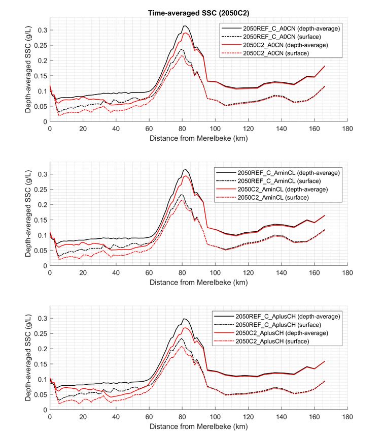
Integraal Plan Bovenzeeschelde - Sub report 18 – Effect of the C-alternatives on mud transport

4.2 Polygons and transects
For analysing the effects of the C-alternatives, a set of new polygons and transects are created for aggregating
the results along the Scheldt Estuary. The polygons are defined together the University of Antwerp in order
to fit the set-up of their ecological system model (Bi et al. 2020b). The transects used in the analysis are the
shared edges between two adjacent polygons along the main channel.
The new polygons for the C alternatives are based on the previous polygons used for the B alternatives. The
new polygons from the North Sea to the Rupel remain the same as before, since the C alternatives only
consist of new measures upstream of Rupel. Although these polygons are kept the same, their numbers can
change according to the polygons added/removed/merged in the upstream.
In the C-alternatives, there are 74 polygons covering the main channel from Vlissingen to the upstream
boundary at Merelbeke. Although for each C alternatives, some of the polygons may have slight different
shapes, the total number is always the same. Moreover, most of the transects between these polygons are
kept the same as in the polygons for the B alternatives. Only few transects are changed slightly in terms of
the angle to the thalweg. Therefore, numbering of polygons in the channel stays the same, and changing
numbering is limited to the “dead-end” systems and the part of the North Sea.
The total number of the new measures, especially the new depoldered areas, FCA-CRT areas, differ from
each other in the C alternatives, therefore, the numbering of these areas, unlike the polygons for the main
channels, is different in each case. The new polygons for the 2050REF_C runs are shown in Figure 20 -
Figure 23. The rest of the polygons used in the C1-C2-C3 alternative runs are shown in the
Appendix 1 Polygons for ΔSSC calculation.

 Figure 20 – Polygons for 2050_REF_C (polygons 1-13, 87-88)

 Final version WL2021R13_131_18 21
Integraal Plan Bovenzeeschelde - Sub report 18 – Effect of the C-alternatives on mud transport

 Figure 21 – Polygons for 2050_REF_C (polygons 13-31, 85-86)

 Figure 22 – Polygons for 2050_REF_C (polygons 32-58, 78-84)

 22 WL2021R13_131_18 Final version
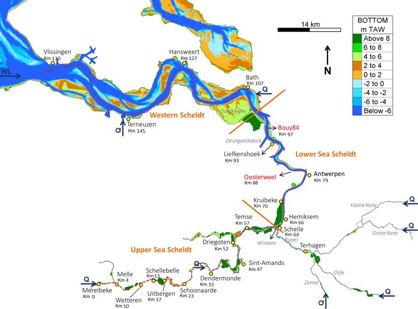
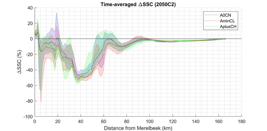
Integraal Plan Bovenzeeschelde - Sub report 18 – Effect of the C-alternatives on mud transport

 Figure 23 – Polygons for 2050_REF_C (polygons 59-77)

In this report, the thalweg distance is defined as the distance from Merelbeke near the upstream boundary.
Therefore, the polygon number (indicated with red numbers in Figure 20 - Figure 23) is converted into the
distance from Merelbeke based on the thalweg defined by the dotted line in Figure 24. The centroid point in
each polygon is used when measuring the distance to Merelbeke. The distance of a transect to the Merelbeke
is defined in a similar way based on the thalweg in Figure 24.

 Figure 24 – Map of the Scheldt estuary with main tributaries and most important locations.
 The thalweg is indicated with the red dotted line.

 Final version WL2021R13_131_18 23
Integraal Plan Bovenzeeschelde - Sub report 18 – Effect of the C-alternatives on mud transport

4.3 Tidal Asymmetry
An important factor that could cause residual sediment transport in estuaries is tidal asymmetry. In the
Western Scheldt it is a principal factor influencing the sediment exchange between the ebb tidal delta and
the estuary, as well as between the various part of the estuary (Wang et al., 1999). Eulerian asymmetries
(Friedrichs, 2011) are determined based on local (point) variations of velocity and water level. For better
interpreting the effects found in the mud model, the tidal asymmetry based on duration of flood-period and
ebb-period is calculated and used in this report:
 flood
 ebb
With Tebb = duration of ebb flow during the tidal cycle and Tflood = duration of flood flow during the tidal cycle.
The duration of ebb and flood flow is computed based on the cross-sectionally averaged velocity at each
transects along the Scheldt estuary

4.4 Delta SSC (ΔSSC)
Three models that are downstream in the modelling chain (ecosystem, fish and bird model) take either
surface or depth-averaged SSC as an input. The modelling chain is explained in more detail in Smolders et al.
(2018). These models are termed ‘subsequent models’ further in the text.
The methodology of working with Deltas as shown in Figure 25 comes down to the simple notion that we
don’t pass the modelled concentrations in the different scenarios on to the subsequent models, but that we
rather calculate the relative effect of a change in bathymetry and/or boundary conditions in a dimensionless
measure Δ. This dimensionless measure is then used to perturb the measured data that was used in setting
up a subsequent model to take into account the expected effect in change of SSC.

 Figure 25 – Methodology of working with Deltas

In the ecological system (ES) model, the surface SSC changes are more relevant since it affects the light
saturation in the water, hence the primary production. In this case, the surface ΔSSC is computed. For the
fish model, the depth-averaged SSC becomes more important than the surface SSC. Hence, we choose to
calculate both the surface delta’s and depth-averaged delta’s over the spatial extent of the boxes in the
ecosystem model.

 24 WL2021R13_131_18 Final version
You can also read