A new global grid-based weighted mean temperature model considering vertical nonlinear variation
←
→
Page content transcription
If your browser does not render page correctly, please read the page content below

Atmos. Meas. Tech., 14, 2529–2542, 2021
https://doi.org/10.5194/amt-14-2529-2021
© Author(s) 2021. This work is distributed under
the Creative Commons Attribution 4.0 License.

A new global grid-based weighted mean temperature model
considering vertical nonlinear variation
Peng Sun1 , Suqin Wu1,2 , Kefei Zhang1,2 , Moufeng Wan1 , and Ren Wang1
1 School   of Environment Science and Spatial Informatics, China University of Mining and Technology, Xuzhou 221116, China
2 SPACE    Research Center, School of Science, RMIT University, Melbourne 3001, Australia

Correspondence: Suqin Wu (sue.wu2018@gmail.com)

Received: 8 July 2020 – Discussion started: 7 October 2020
Revised: 12 February 2021 – Accepted: 19 February 2021 – Published: 31 March 2021

Abstract. Global navigation satellite systems (GNSS) have         and 3.94 K, respectively. Compared to the second reference,
been proved to be an excellent technology for retrieving pre-     the mean bias and mean RMSE of the model-predicted Tm
cipitable water vapor (PWV). In GNSS meteorology, PWV             values over the 428 radiosonde stations at the surface level
at a station is obtained from a conversion of the zenith wet      were 0.34 and 3.89 K, respectively; the mean bias and mean
delay (ZWD) of GNSS signals received at the station using         RMSE of the model’s Tm values over all pressure levels in the
a conversion factor which is a function of weighted mean          height range from the surface to 10 km altitude were −0.16
temperature (Tm ) along the vertical direction in the atmo-       and 4.20 K, respectively. The new model results were also
sphere over the site. Thus, the accuracy of Tm directly af-       compared with that of the GTrop and GWMT_D models in
fects the quality of the GNSS-derived PWV. Currently, the         which different height correction methods were also applied.
Tm value at a target height level is commonly modeled us-         Results indicated that significant improvements made by the
ing the Tm value at a specific height and a simple linear de-     new model were at high-altitude pressure levels; in all five
cay function, whilst the vertical nonlinear variation in Tm is    height ranges, GGNTm results were generally unbiased, and
neglected. This may result in large errors in the Tm result       their accuracy varied little with height. The improvement in
for the target height level, as the variation trend in the ver-   PWV brought by GGNTm was also evaluated. These results
tical direction of Tm may not be linear. In this research, a      suggest that considering the vertical nonlinear variation in Tm
new global grid-based Tm empirical model with a horizontal        and the temporal variation in the coefficients of the Tm model
resolution of 1◦ × 1◦ , named GGNTm, was constructed us-          can significantly improve the accuracy of model-predicted
ing ECMWF ERA5 monthly mean reanalysis data over the              Tm for a GNSS receiver that is located anywhere below the
10-year period from 2008 to 2017. A three-order polynomial        tropopause (assumed to be 10 km), which has significance
function was utilized to fit the vertical nonlinear variation     for applications requiring real-time or near real-time PWV
in Tm at the grid points, and the temporal variation in each      converted from GNSS signals.
of the four coefficients in the Tm fitting function was also
modeled with the variables of the mean, annual, and semi-
annual amplitudes of the 10-year time series coefficients.
The performance of the new model was evaluated using its          1   Introduction
predicted Tm values in 2018 to compare with the following
two references in the same year: (1) Tm from ERA5 hourly          Water vapor, as an important greenhouse gas, is closely re-
reanalysis with the horizontal resolution of 5◦ × 5◦ ; (2) Tm     lated to weather variations; hence, it is crucial to monitor the
from atmospheric profiles from 428 globally distributed ra-       water vapor content in the atmosphere for a reliable weather
diosonde stations. Compared to the first reference, the mean      forecast. The meteorological parameter that is closely re-
RMSEs of the model-predicted Tm values over all global            lated to water vapor is precipitable water vapor (PWV) and
grid points at the 950 and 500 hPa pressure levels were 3.35      it can be measured by various technologies such as radioson-
                                                                  des, remote-sensing satellites, and water vapor radiometers.

Published by Copernicus Publications on behalf of the European Geosciences Union.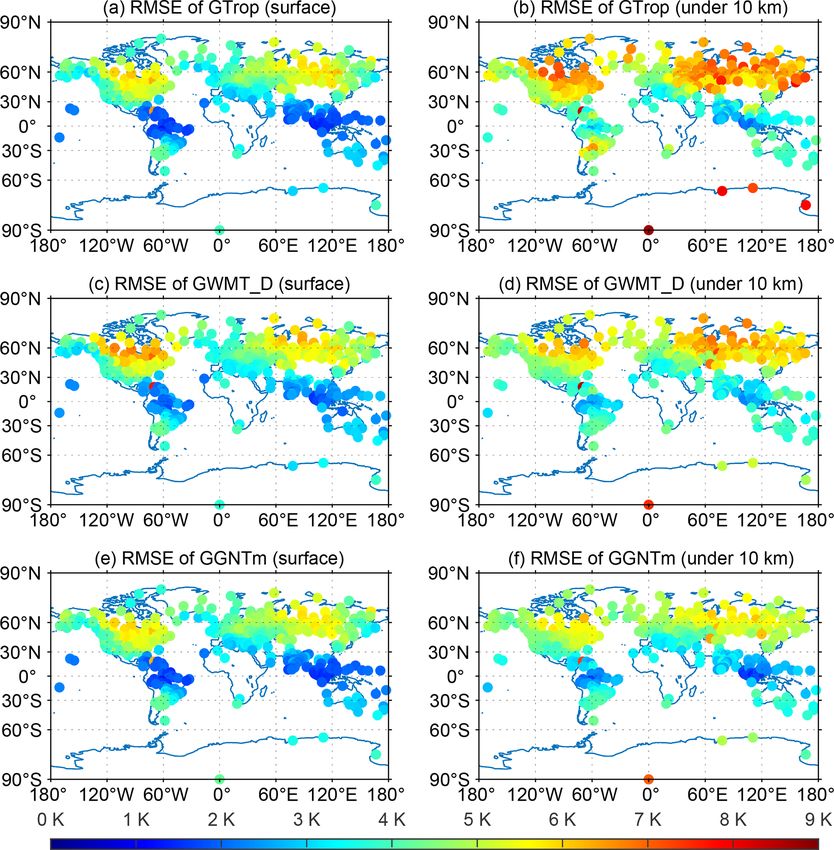
2530                                              P. Sun et al.: A new global grid-based weighted mean temperature model

Global navigation satellite systems (GNSS), which were ini-       temperature over the GNSS site, which is defined and
tially designed for positioning, navigation, and timing, can      approximated through the following equation (Davis et al.,
be used to retrieve the zenith tropospheric delay (ZTD) of        1985):
the GNSS signal over an observation station. The ZTD can                          Pn e i
                                                                                    1 T 1hi
                                                                         R e
be divided into zenith hydrostatic delay (ZHD) and zenith                    dh
                                                                  Tm = R Te     ≈ Pn e i    ,                           (3)
wet delay (ZWD). The ZHD can usually be obtained at a                     T2
                                                                             dh        i
                                                                                    1 2 1hi
high accuracy from the Saastamoinen model together with                                   Ti

measured meteorological data at the station. The atmospheric      where e and T are the water vapor pressure (hPa) and abso-
water vapor information is contained in the GNSS-ZTD –            lute temperature (K), respectively; n is the number of the lay-
more precisely, in the GNSS-ZWD – which can be con-               ers; ei , T i , and 1hi are the mean water vapor pressure, mean
verted into PWV. Different from the other atmospheric mea-        temperature, and thickness of the ith layer, respectively.
surement techniques, GNSS receivers are regarded as cost-             From Eq. (2), one can see that Tm is a crucial variable
effective equipment for meteorological research; the main         for the determination of the conversion factor 5, which in
advantage of the GNSS-based method is its real-time, stable,      turn affects the determination of PWV expressed by Eq. (1).
high temporal-resolution, and relative long-term capabilities.    The significance of obtaining accurate Tm values has been
The GNSSs were first applied to meteorological research in        demonstrated by previous research (Bevis, 1994; Jiang et al.,
the 1990s (Bevis et al., 1992). Some preliminary research in      2019a; Ning et al., 2016; Wang et al., 2005, 2016). Tm can
relation to the long-term feature of the GNSS-ZTD/PWV se-         be calculated from an observed atmospheric profile. This ob-
ries and the relationship between GNSS-PWV and weather            served atmospheric profile can be acquired from a radiosonde
or climate issues has already been carried out (Bianchi et al.,   station, which is valid only for the sounding site. In fact, for
2016; Bonafoni and Biondi, 2016; Calori et al., 2016; Chen        GNSS stations, they are usually not co-located with any re-
et al., 2018; Choy et al., 2013; He et al., 2019; Shi et al.,     gional radiosonde stations; i.e., observed atmospheric pro-
2015; Rohm et al., 2014a; Wang et al., 2016, 2018; Zhang          files are unavailable. As a result, Eq. (3) is not applicable
et al., 2015). Near real-time GNSS-ZTD products estimated         for GNSS stations. Moreover, even if a GNSS station is co-
from GNSS data processing have been routinely assimilated         located with a radiosonde station, due to the low temporal
into numerical weather models (NWMs) for improving the            and spatial resolution of radiosonde data, the temporal reso-
performance of weather forecasts (Bennitt and Jupp, 2012;         lution of its resultant Tm is also low, which cannot meet the
Dousa and Vaclavovic, 2014; Guerova et al., 2016; Le Mar-         requirements of GNSS near real-time or real-time (NRT/RT)
shall et al., 2012, 2019).                                        applications such as the conversion of GNSS-ZWD time se-
   To obtain GNSS-PWV over a station, the first step is to        ries into PWV time series. The atmospheric profiles from
estimate the ZTD of the station from GNSS data process-           NWM data can be obtained for Tm determination (Wang et
ing, and the two most common data processing strategies are       al., 2005, 2016). However, for some time-critical applica-
the network approach and precise point positioning (PPP) ap-      tions, NRT/RT Tm is essential for NRT/RT GNSS-PWV de-
proach (Ding et al., 2017; Douša et al., 2016; Guerova et al.,    termination; thus the main drawback in using the reanalysis
2016; Li et al., 2015; Lu et al., 2015; Rohm et al., 2014b;       data is its latency issue, and it is still difficult for most users to
Yuan et al., 2014; Zhou et al., 2020). The former uses double-    obtain predicted results to obtain from the NWM data. Thus,
differenced observations, while the latter uses un-differenced    it is of great importance to develop empirical Tm models for
observations in the observation equation system. The ZWD          time-critical applications. Some Tm models have been devel-
can be obtained from subtracting the ZHD from the GNSS-           oped with a focus of improving the accuracy of the Tm , and
ZTD or directly estimated if the ZHD has been corrected           these empirical models can be classified into two categories.
in the GNSS observation equation system, depending on the         One category is such a model that depends on in situ surface
processing strategies adopted. Then the GNSS-PWV can be           temperature observation Ts , like the Bevis model, which is
converted by                                                      a simple linear function expressed as Tm = a + bTs (Bevis
                                                                  et al., 1992). The two coefficients of such a linear function
PWV = 5 × ZWD,                                             (1)    can be determined from the linear regression method based
where 5 is the conversion factor (Askne and Nordius, 1987;        on long-term regional radiosonde data. However, the deploy-
Bevis et al., 1992), which is given by                            ment of radiosonde stations is geographically sparse due to
                                                                  their high cost, and it is even worse that there are no ra-
              106                                                 diosonde stations at all in some areas. One of the possible
5=                            ,                            (2)
       ρw Rv ( Tkm3 + k20 )                                       ways to solve the availability issue is to use reanalysis data
                                                                  to develop Tm −Ts models. However, such a reanalysis-based
where ρw is the density of liquid water; Rv =                     Tm −Ts model may not be as accurate as that derived from lo-
461.5 J/(kg × K) is the specific gas constant for water           cal radiosonde profiles. Yao et al. (2014a) developed a global
vapor; k20 = 22.1 K/hPa and k3 = 373900 K2 /hPa are at-           latitude-dependent Tm –Ts linear model using Tm data from
mospheric refractivity constants; Tm is the weighted mean         the global geodetic observing system (GGOS) and Ts data

Atmos. Meas. Tech., 14, 2529–2542, 2021                                              https://doi.org/10.5194/amt-14-2529-2021
P. Sun et al.: A new global grid-based weighted mean temperature model                                                            2531

from the European center for medium-range weather fore-
casts (ECMWF). Jiang developed a time-varying global grid-
ded Tm –Ts model using both Tm and Ts derived from ERA-
Interim (Jiang et al., 2019a). Ding (2018, 2020) developed
two generations of global Tm models using the neural net-
work algorithm, in which temperature observations were re-
quired for the input and the models performed well. The Tm
models mentioned above need in situ meteorological obser-
vations (mainly Ts ) as the model’s input. However, for GNSS
stations, not all stations are equipped with meteorological
sensors. Although the meteorological parameters at the user
station can also be interpolated using the actual meteorologi-
cal measurements nearby, the interpolation error depends on
the terrain difference between the meteorological sensor’s lo-
cation and the point of interest in addition the interpolation
methods used.
   To address the above-mentioned issues, the type of empir-
ical models that are independent of meteorological observa-
tions had to be constructed. Yao et al. (2014b, 2012, 2013)
used spherical harmonics to develop the GWMT, GTM-II,
and GTM-III models, in which both the height and the peri-
odicity of Tm were taken into account. Huang et al. (2019a)        Figure 1. Temperature T , water vapor pressure e, and Tm profiles
established a global Tm model using the sliding window algo-       obtained from ERA5 monthly mean reanalysis in December 2017
                                                                   at four grid points: (a) 90◦ N, 120◦ E; (b) 60◦ N, 120◦ E; (c) 30◦ N,
rithm, which was based on varying latitude and altitude. The
                                                                   120◦ E; (d) 0◦ N, 120◦ E.
widely used GPT2w model (Böhm et al., 2015) and its suc-
cessor, GPT3 (Landskron and Böhm, 2018), provided grid-
ded results with both 1◦ × 1◦ and 5◦ × 5◦ horizontal reso-         discussed, considering the lapse rate in a Tm model can im-
lutions, and the models also contain a few terms related to        prove the model’s accuracy. However, the assumption that
temporal variations in Tm including the mean, annual, and          Tm linearly varies with height, which many recently devel-
semi-annual amplitudes. However, the height differences be-        oped models were based on, may not agree well with the
tween the user site, e.g., a GNSS station, and its nearest four    truth. In this research, a new global grid-based empirical Tm
surrounding grid points were not considered. Recent studies        model, named GGNTm, in which the vertical nonlinear vari-
have overcome this problem by providing Tm values at var-          ation in Tm was taken into account, was developed using a
ious heights ranging from ground surface to the upper tro-         three-order polynomial function and ERA5 monthly mean
posphere. He et al. (2017) developed a voxel-based global          reanalysis data over the 10-year period from 2008 to 2017,
model, named GWMT-D, using the Tm values at four height            and the temporal variation in each of the four coefficients in
levels of reanalysis data from the National Centers for En-        the Tm fitting function was also modeled with the variables of
vironmental Prediction (NCEP) to construct the voxels. The         the mean, annual, and semi-annual amplitudes of the 10-year
Tm predicted for the user site can be obtained from an inter-      time series coefficient.
polation of the Tm values at the eight grid points of the voxel       The outline of the paper is as follows. The features of
that contains the user site. In recent studies, some researchers   the vertical nonlinear variation in Tm were investigated in
used a Tm lapse rate, the rate of change in Tm with altitude, to   Sect. 2.2; then a three-order polynomial function fitting the
correct the effect of the height element on Tm , e.g., IGPT2w      10-year Tm profiles obtained from ERA-5 monthly mean
(Huang et al., 2019b), GTm_R (Li et al., 2020), and GPT2wh         reanalysis data was developed for the GGNTm model. In
(Yang et al., 2020). The GTrop model (Sun et al., 2019), de-       Sect. 3, the performance of GGNTm was validated using the
veloped for predicting both ZTD and Tm , also took into ac-        Tm values from ERA5 hourly reanalysis and globally dis-
count the Tm lapse rate, and it outperforms GPT2w obviously        tributed radiosonde profiles in 2018 as the references. Con-
at altitudes under 10 km.                                          clusions are summarized in the final section.
   We have noticed that some studies have extended the
GNSS-PWV sensing to a shipborne GNSS receiver or GNSS
receiver that is onboard other moving vehicles (Fan et al.,
2016; Wang et al., 2019; Webb et al., 2016). Thus, we con-
centrated on developing a high-accuracy unbiased empiri-
cal model for predicting Tm values in any possible places,
which is meaningful for GNSS meteorology. As previously

https://doi.org/10.5194/amt-14-2529-2021                                              Atmos. Meas. Tech., 14, 2529–2542, 2021
2532                                                P. Sun et al.: A new global grid-based weighted mean temperature model

Figure 2. Mean of rms’s of the Tm residuals of 120 monthly mean profiles from the 10-year period at each grid point for scheme 1 (a, for
linear function) and scheme 2 (b, for three-order polynomial function).

2     Methodology for new model construction                          grid points obtained from ERA5 monthly mean reanalysis in
                                                                      December 2017. It should be noted that the surface heights
2.1    Data source                                                    of the four grid points were different, and they were 0, 301,
                                                                      13, and 180 m, respectively. Panels (a) and (b) show that, in
ERA5 reanalysis data were the latest reanalysis data de-              the height range near the surface, temperature increases with
veloped by the ECMWF. In this research, ERA5 monthly                  the increase in height. In addition, all the four Tm profiles
mean reanalysis data in the 10-year period from 2008 to               (the black curves with dots) in these panels show a nonlin-
2017 containing geopotential heights, temperatures, and spe-          ear variation trend. This implies that using a constant lapse
cific humidity at 37 pressure levels with a horizontal resolu-        rate to model the vertical Tm variation trend will result in
tion of 1◦ × 1◦ were downloaded from the web server of the            large errors; i.e., the Tm profiles cannot be accurately mod-
Copernicus Climate Change Service (C3S). The geopotential             eled through a constant Tm lapse rate. This finding aligns well
heights, which are often used in meteorology, were then con-          with that of other researchers (e.g., Yao et al., 2018).
verted to WGS-84 ellipsoidal heights. Water vapor pressure
was calculated by (Nafisi et al., 2012)                               2.3   Three-order polynomial function for Tm vertical
e = qp/(0.622 + 0.378q),                                      (4)           fitting

where q is the specific humidity, which can be obtained from          A linear Tm decay function with a constant Tm lapse rate can
NWM data; p is the atmospheric pressure.                              be expressed as

2.2    Vertical variation in Tm                                       Tm = α + β(H − h0 ),                                          (5)

The ERA5 monthly mean products were used to analyze the               where α is the Tm value at the reference height h0 ; β is the
vertical variation in Tm . As defined in Eq. (3), Tm is a func-       Tm lapse rate and H is the ellipsoidal height (km) of the user
tion of water vapor pressure and temperature. The variation           site. An equivalent expression of Eq. (5) is
in water vapor pressure in the vertical direction has been
known to be nonlinear, while the vertical variation in temper-        Tm = α 0 + β 0 H,                                             (6)
ature is often assumed to be a linear decay function (Dousa
and Elias, 2014). In fact, there is such a phenomenon that            where α 0 denotes the Tm value at 0 km ellipsoidal height.
temperature increases with the increase in height, the so-            Some Tm models were constructed based on this linear Tm
called temperature inversion, which occurs in both the upper          decay function. Tm values from different height ranges can
atmosphere and near ground surface, meaning that the ver-             be used to calculate the Tm lapse rate. However, if Tm varies
tical variation in temperature is complex. As a result, Tm in         nonlinearly in the vertical direction, the calculated Tm lapse-
the vertical direction varies nonlinearly due to the irregular        rate values would have large errors. To overcome this prob-
variations in both water vapor pressure and temperature in            lem, in this research, a three-order polynomial function was
the vertical direction. Figure 1 shows four vertical profiles         selected for a new Tm model:
of water vapor pressure, temperature, and Tm at the pres-
sure levels that were under a 10 km ellipsoidal height at four        Tm = a + bH + cH 2 + dH 3 ,                                   (7)

Atmos. Meas. Tech., 14, 2529–2542, 2021                                                   https://doi.org/10.5194/amt-14-2529-2021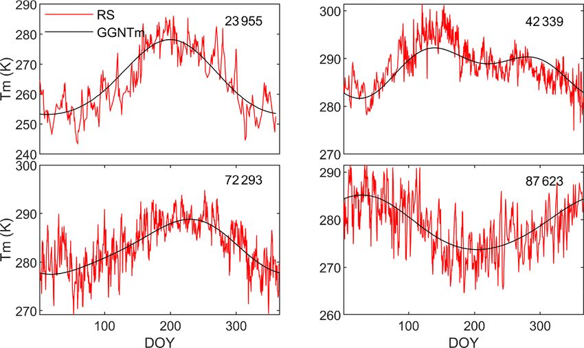
P. Sun et al.: A new global grid-based weighted mean temperature model                                                                    2533

Figure 3. Periodicity reflected in the 10-year time series of each coefficient in the three-order polynomial function at 60◦ N, 120◦ E.

where a, b, c, d are the four unknown coefficient parameters
of the fitting function.
   For the estimation of the two sets of unknown coeffi-
cient parameters expressed in Eqs. (6) and (7), two schemes,
named scheme 1 and scheme 2, fitted the sample data of Tm
profiles of the 120 monthly mean reanalysis data over the 10-
year period from 2008 to 2017 at each grid point for the two
functions. It should be noted that only those Tm values from
heights under 10 km were selected for the sample data. For
measuring how well the fitting function fits the sample data,
the root mean square (rms) of the differences between the Tm
values resulting from the fitting function and the sample data
was calculated by
        v
        u n
        u1 X 2
rms = t          1i ,                                      (8)            Figure 4. Spatial interpolation of the Tm value for the target point
            n i                                                           (ϕλH ). After obtaining the Tm values at height H at the four grid
                                                                          points (see the four grids on the top plane) by the GGNTm model
where 1i is the residual of Tm at the ith pressure level over             using Eq. (7), the Tm value at the target point can be interpolated
the grid point. Figure 2 shows the map for the mean of the                (the dashed rectangle).
rms’s of the fitting residuals of the Tm from the aforemen-
tioned 120 monthly mean Tm profiles (the samples) at each
of the grid points. The mean of the mean rms’s at all global              2.4   Tm temporal fitting for the new model
grid points for scheme 1 and scheme 2 were 1.26 and 0.30 K,
respectively. In addition, the rms results in panel (a) (for lin-         In the previous section, the 10-year time series of coefficients
ear function) were latitude-dependent, and small rms’s (blue)             in the three-order polynomial function expressed in Eq. (7) at
were in midlatitude regions; large rms values in both panels              each of the grid points were obtained from the least-squares
were in Antarctica. Comparing the two panels, we found that               estimation. Since they were not constant values, the tem-
the rms values shown in panel (b) were all very small and                 poral variation in each coefficient at each grid point needs
significantly smaller than those of panel (a), meaning that               to be further modeled for the new grid-based empirical Tm
the three-order polynomial fitting function was superior to               model proposed in this study, GGNTm. The seasonal vari-
the linear fitting function.                                              ation reflected in the 10-year time series of each of the co-

https://doi.org/10.5194/amt-14-2529-2021                                                     Atmos. Meas. Tech., 14, 2529–2542, 2021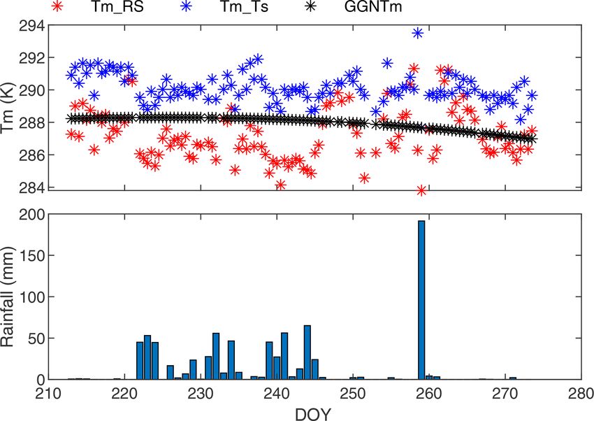
2534                                                    P. Sun et al.: A new global grid-based weighted mean temperature model

Table 1. Mean bias and mean RMSE of Tm values at each of five pressure levels at 12:00 UTC at all global grid points in 2018 resulting from
each of the three models selected.

                                 Pressure level (hPa)     Statistic (K)                  Model
                                                                          GTrop      GWMT_D        GGNTm
                                 950
                                                          mean bias       −0.14             1.68     −0.43
                                                          mean RMSE        3.39             3.98      3.35
                                 800
                                                          mean bias       −0.14             2.09       0.09
                                                          mean RMSE        3.79             4.46       3.77
                                 650
                                                          mean bias           0.76          1.84       0.15
                                                          mean RMSE           4.14          4.58       4.07
                                 500
                                                          mean bias           2.97          2.07       0.30
                                                          mean RMSE           5.17          4.57       3.94
                                 350
                                                          mean bias           5.71          1.90       0.78
                                                          mean RMSE           7.12          3.93       3.02

efficients r = a, b, c, d was analyzed using the fast Fourier                 2. use Eq. (7) to calculate the Tm values at the height of the
transform (FFT), and results for seasonality and periodicity                     user site at each of the above four grid points (which is
at point 60◦ N, 120◦ E are shown in Fig. 3, which presented                      for the height dimension);
noticeable annual and semi-annual amplitudes. Similar pe-
riodicities were also found at other grid points. According
to these characteristics, the fitting model for GGNTm con-                    3. use an interpolation method, such as the inverse distance
taining three terms including mean, annual, and semi-annual                      weighting or bilinear interpolation, on the four Tm val-
amplitudes for each coefficient time series at each grid point                   ues from step (2) to obtain the Tm value for the user
expressed by the following was adopted in this study:                            site (which is for the horizontal dimension, as shown in
                                                                                 Fig. 4).
                   doy − d1                doy − d2
r = A0 + A1 cos(            2π ) + A2 cos(          4π ), (9)               Till now the new model has been developed based on the
                    365.25                  365.25
                                                                          10-year sample data from 2008 to 2017. This model will be
where A0 , A1 , and A2 are the mean, annual, and semi-annual              validated using the model-predicted Tm results in 2018 com-
amplitudes, respectively; doy denotes “day of year”; d1 and               pared against the same year’s (i.e., out-of-sample) reference
d2 are the initial phases of the annual and semi-annual pe-               data. Results will be discussed in the next section.
riodicities, which are estimated together with the mean and
amplitudes.
   Then, the mean, annual, and semi-annual amplitudes and
initial phases for each coefficient at each of the grid points            3    Evaluation of GGNTm
over the globe (with the resolution of 1◦ × 1◦ ) were deter-
mined using the least-squares estimation method and the 10-               For the performance assessment of our newly developed Tm
year time series of the coefficient. To calculate Tm for a spe-           model, Tm values over different pressure levels obtained from
cific site and time, e.g., for a GNSS station at an observing             both ERA-5 hourly reanalysis (at 12:00 UTC) and globally
time, the following three-step procedure needs to be carried              distributed radiosonde profiles in 2018 were selected as the
out:                                                                      references. Thus, both 24 and 12 h variations in Tm have been
                                                                          contained in the reference data for the evaluation of our new
  1. use Eq. (9) to calculate each of the four coefficients at            model. The two statistics – bias and RMSE – were utilized to
     each of the four grid points surrounding the user site;              measure the systematic discrepancy and the accuracy of the

Atmos. Meas. Tech., 14, 2529–2542, 2021                                                      https://doi.org/10.5194/amt-14-2529-2021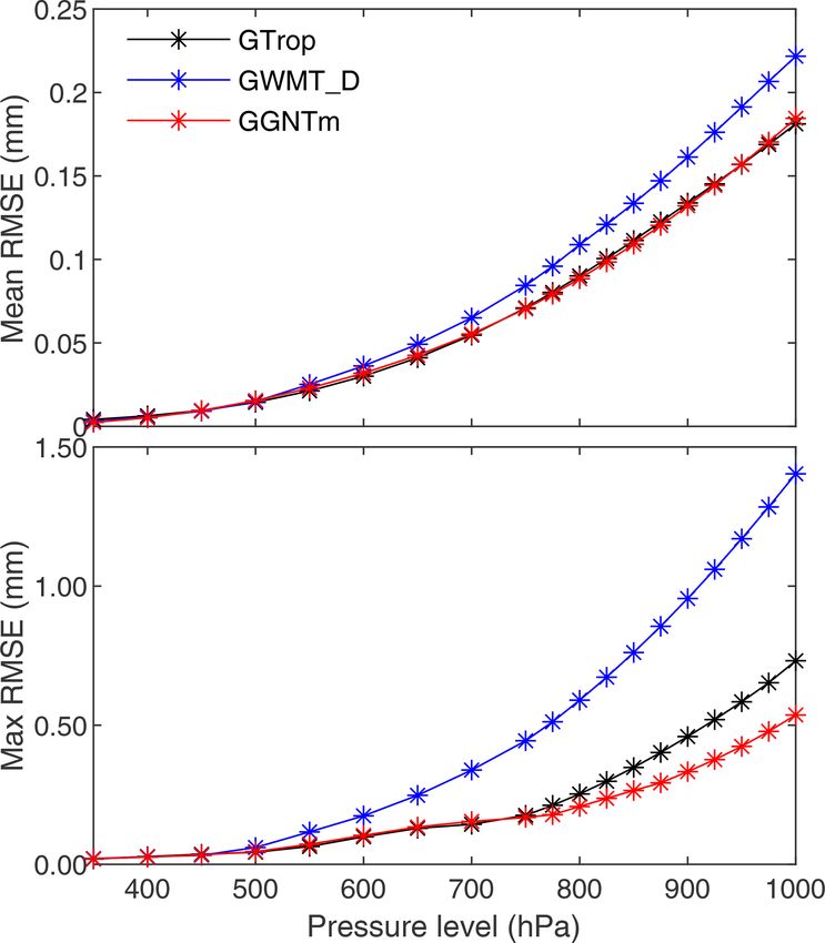
P. Sun et al.: A new global grid-based weighted mean temperature model                                                            2535

Figure 5. RMSE of Tm at each grid point at 950 hPa (a, c, e) and 500 hPa (b, d, f) pressure levels in 2018 resulting from GTrop, GWMT_D,
and GGNTm.

model results. Their formulas are                                     pressure levels: 950, 800, 650, 500, and 350 hPa were used to
                                                                      calculate the bias and RMSE of the new model’s Tm results
        n
     1X                                                               at the pressure level. In addition to the GGNTm model, the
bias =    (T model − Tmrefi ),                              (10)
     n i=1 mi                                                         other two empirical models developed in recent years includ-
       v
       u n                                                            ing GTrop and GWMT_D, in which different vertical cor-
       u 1 X model                                                    rection methods were also applied, were also evaluated for
RMSE = t       (T        − Tmrefi )2 ,                      (11)
          n i=1 mi                                                    performance comparisons of GGNTm and these two models.
                                                                         Table 1 shows the mean bias and mean RMSE of the
                                                                      Tm values over all global grid points resulting from each of
where i is the index of the data element; Tmmodel      denotes
                                                 i                    the above three models. As we can see, on a global scale,
the model resultant Tm value; Tmrefi denotes the reference Tm         GGNTm outperformed all the other two models, especially
value; n is the number of the Tm values in the statistics.            at high pressure levels. The GTrop has been proved to be
                                                                      considerably better than GPT3 (Sun et al., 2019), owing to
3.1   Comparison with ERA5 hourly data
                                                                      its use of the Tm lapse rate, although its Tm results still had
                                                                      large errors at high pressure levels, which is most likely to
As the first set of the reference selected for the evaluation of
                                                                      result from neglecting the nonlinear vertical variation in Tm .
the new model, ERA-5 hourly data (with the resolution of
                                                                      The large bias and RMSE of the GWMT_D results were pos-
5◦ × 5◦ ) at 12:00 UTC on each day in 2018, which were out-
                                                                      sibly because its modeling was based on NCEP reanalysis
of-sample data, were downloaded from the C3S. Then they
                                                                      data, and there may exist differences between the reanalysis
were converted to Tm profiles and Tm values at each of five

https://doi.org/10.5194/amt-14-2529-2021                                                 Atmos. Meas. Tech., 14, 2529–2542, 2021
2536                                                P. Sun et al.: A new global grid-based weighted mean temperature model

Figure 6. Tm values (at the earth surface) integrated from the radiosonde measurements as well as that predicted by GGNTm at each of the
four radiosonde stations (nos. 23955, 42339,72293, and 87623).

data from ECMWF and NCEP (Chen et al., 2011; Decker                   sure level from a radiosonde profile was calculated through a
et al., 2012). Compared to GTrop and GWMT_D, GGNTm                    mixing ratio:
performed very well at all pressure levels. This is because the
model accounted for the vertical nonlinear variation in Tm .          e = Rp/(622 + R),                                            (12)
   The results shown in Table 1 were the statistics of all            where R denotes the mixing ratio (g/kg).
global grid points at each of the five pressure levels selected.         An additional data pre-processing procedure needs to be
For more refined results, Fig. 5 shows the map for the RMSE           conducted for data quality control. Those poor radiosonde
of Tm at each grid point at either the 950 or 500 hPa pres-           profiles needed to be identified and excluded from their use
sure levels resulting from three models. The 950 hPa pressure         for the reference. The first check was for a valid mixing ratio
level (Fig. 5a, c, e) results indicated that the RMSEs of Tm          value: if a pressure level lacks a valid mixing ratio value, then
resulting from all the three models were latitude-dependent           it is regarded as invalid and thus to be excluded. After this
and high-accuracy Tm values (in blue) were mainly in low-             initial checking was performed, further identifications were
latitude belts. However, the results at the 500 hPa pressure          also carried out. A profile would be excluded if it met any
level (Fig. 5b, d, f) indicated that the new model signifi-           one of the following four conditions:
cantly outperformed the other two models. In addition, from
the 950 hPa pressure level results, the percentages of those            1. the profile lacks surface meteorological observations;
RMSE values that were under 5 K from all the global grid
                                                                        2. the pressure value of the top pressure level is greater
points for GTrop, GWMT_D, and GGNTm were 93.4 %,
                                                                           than 100 hPa;
82.1 %, and 94.6 %, respectively; while the corresponding
percentage values at the 500 hPa level were 44.9 %, 70.6 %,             3. the difference in the pressure values at two successive
and 88.7 %. These suggest that larger improvements made                    levels is under 200 hPa;
by the new model, i.e., GGNTm, over the other two models
were at high-altitude pressure levels.                                  4. the profile consists of a few pressure levels; e.g., if
                                                                           1P /n ≤ 30 hPa (where 1P is the difference of the
                                                                           pressure values at the surface and the 100 hPa pressure
3.2    Comparison with radiosonde data
                                                                           levels and n is the number of all pressure levels from the
                                                                           surface to the 100 hPa pressure levels), then the profile
In this section, Tm from radiosonde profiles were used as the
                                                                           was regarded to have sufficient number of pressure lev-
reference for the performance assessment of the models se-
                                                                           els; otherwise it would be excluded from the use in the
lected. The original radiosonde data at all globally distributed
                                                                           testing.
stations in 2018 were downloaded from the website of the
University of Wyoming (http://weather.uwyo.edu/upperair/,                Sounding balloons are commonly launched twice a day
last access: 13 March 2020). Different from the use of reanal-        (at 00:00 and 12:00 UTC). In this research, only those sta-
ysis data as the reference, water vapor pressure at each pres-        tions that had at least 300 profiles in 2018 were selected in

Atmos. Meas. Tech., 14, 2529–2542, 2021                                                 https://doi.org/10.5194/amt-14-2529-2021
P. Sun et al.: A new global grid-based weighted mean temperature model                                                                  2537

Table 2. Mean bias and mean RMSE of Tm values at 428 globally distributed radiosonde stations in 2018 resulting from GPT3, GTrop,
GWMT_D, and GGNTm.

                             Height             Model                             Bias (K)                 RMSE (K)
                             Surface
                                                GPT3             −0.36 [−7.87         5.81]         3.97 [1.36 12.51]
                                                GTrop             0.16 [−2.39         4.23]          3.87 [1.35 7.22]
                                                GWMT_D            1.30 [−1.74         5.64]          4.07 [1.51 7.81]
                                                GGNTm            −0.34 [−3.17         3.74]          3.89 [1.39 7.03]
                             Under 10 km
                                                GPT3              22.00 [6.78 27.29]              27.67 [10.80 33.53]
                                                GTrop             1.50 [−3.68 5.97]                  5.08 [1.90 8.68]
                                                GWMT_D            1.16 [−0.20 6.18]                  4.61 [2.24 8.52]
                                                GGNTm            −0.16 [−3.81 4.69]                  4.20 [1.37 7.30]

                           Note: the values within square brackets are the minimum and maximum.

Figure 7. RMSE of Tm at surface level (a, c, e) and all pressure levels under 10 km (b, d, f) at each of the 428 radiosonde stations in
2018 resulting from GTrop, GWMT_D, and GGNTm. The RMSE of Tm under 10 km was calculated using the differences between model-
predicted Tm values and the Tm values over all pressure levels with a height of less than 10 km.

https://doi.org/10.5194/amt-14-2529-2021                                                              Atmos. Meas. Tech., 14, 2529–2542, 2021
2538 P. Sun et al.: A new global grid-based weighted mean temperature model
the model performance assessment. After the above five-step
quality control procedure was performed, a total of 260 140
profiles from 428 global radiosonde stations were finally
used in the performance evaluation of three selected models.
Figure 6 shows the Tm values (at the earth surface) integrated
from the radiosonde measurements as well as that predicted
by GGNTm at four radiosonde stations.
Table 2 shows the mean bias and RMSE of surface Tm val-
ues and Tm values at all pressure levels from the surface to
10 km height at all the aforementioned radiosonde stations
resulting from each of the three models that were the same
as the ones tested in the previous section. For the surface Tm
results, the mean RMSE of GTrop and GGNTm were very
close; GWMT_D was the worst, with the largest bias and
RMSE values, which may be due to its low horizontal res- Figure 8. Bias and RMSE of Tm from radiosonde profiles at 428
olution (5◦ × 5◦ ). The other set of results, the RMSE of Tm global radiosonde stations in each of five height ranges resulting
under 10 km, was calculated using the differences between from GTrop, GWMT_D, and GGNTm.
model-predicted Tm values and the reference Tm values over
all pressure levels with a height of less than 10 km. A small
RMSE of Tm under 10 km indicates that the model performs the characteristics of the vertical nonlinear variation in Tm
well at any altitudes below the tropopause. As we can see, are modeled by the proposed model more accurately than the
GWMT_D was slightly better than GTrop, possibly because other models.
the Tm value from the former was interpolated from the Tm
3.3 Evaluation of GGNTm under extreme weather
values at four height levels; the mean bias of Tm from the new
conditions
model, GGNTm, was the lowest, with the value of −0.16,
which was close to 0, meaning nearly unbiased; the RMSE The performance of our model under extreme weather con-
of the new model was also the lowest, among the three mod- ditions has also been assessed. The Tm values integrated
els, which suggests that the vertical nonlinear variation in Tm from the radiosonde profiles at KingsPark radiosonde sta-
was modeled more accurately in the new model than in the tion (no. 45005, Hong Kong) from August to September in
other existing models. 2018 (summer storm period) were taken as the reference data
Similar to Fig. 5, Fig. 7 shows the map for the RMSE of in this research. As is shown in Fig. 9, the Tm values at
Tm values at each of the 428 radiosonde stations in 2018 at the station predicted by GGNTm as well as a Tm –Ts model
the surface pressure level (Fig. 5a, c, e) and all pressure lev- (Tm = 0.6195 × Ts + 103.3452) developed using Tm and Ts
els with a height of less than 10 km (Fig. b, d, f) resulting series at KingsPark station (He et al., 2019) were compared
from GTrop, GWMT_D, and GGNTm. It can be found that against corresponding radiosonde measurements during the
the RMSEs of all models were latitude-dependent, and those summer storm period. The daily total rainfall data (pub-
stations that had a large RMSE value were mostly located lished by Hong Kong Observatory, https://www.hko.gov.hk,
in north Africa and northeast America. At the four stations last access: 2 December 2020) during the 2 months are also
located in Antarctic, their surface Tm values were accurately shown in the figure. Heavy rainfall occurred frequently in
modeled by these models. However, in terms of the RMSE of Hong Kong during the 2 months, and a super typhoon, named
all pressure levels under 10 km, the GTrop results were rel- Mangkhut, landed near Hong Kong and caused torrential rain
atively large at the four stations, whilst both GWMT_D and on 16 September. As is shown in the figure, our model shows
GGNTm performed well at three of the stations. clear outperformance during the 2 months compared to the
To further evaluate the performance of the three mod- Tm –Ts model. More experiments showed that the coefficients
els at different height ranges under 10 km, the models’ Tm of Tm –Ts models vary significantly with time (i.e., 0.6195 vs.
values from the aforementioned radiosonde profiles at the 0.58 for the linear part and 103.3452 vs. 115.71 for the con-
428 global stations were divided into five height ranges, and stant part, respectively), which means that a Tm − Ts model
Fig. 8 shows each height range’s bias and RMSE. We can that is based on the linear regression may have large errors
see the following results: (1) in the height ranges above 4 km, during some periods.
the GTrop results had the largest bias and largest RMSE, and
GWMT_D was considerably better than GTrop; (2) in low 3.4 Impact of GGNTm on PWV
height ranges the GWMT_D results were the worst; (3) in all
height ranges the GGNTm results were nearly unbiased and The accuracy of GNSS-PWV over a GNSS site at an ob-
their accuracy varied little with height. The GGNTm model’s serving time is dependent upon the accuracies of the ZWD
consistent high accuracy in all height ranges suggests that and the conversion factor. Uncertainty analysis has been con-
Atmos. Meas. Tech., 14, 2529–2542, 2021 https://doi.org/10.5194/amt-14-2529-2021P. Sun et al.: A new global grid-based weighted mean temperature model 2539
Figure 9. Tm derived from radiosonde profiles, the Tm − Ts model,
GGNTm from August to September in 2018 at KingsPark station,
and the daily total rainfall at Hong Kong International Airport.
ducted by some researchers to study the uncertainty of the
GNSS-derived PWV resulting from different variables, in-
Figure 10. Mean RMSE and maximum RMSE of PWV values at
cluding the uncertainty of GNSS-ZTD, the atmospheric pres-
each of the pressure levels at 12:00 UTC at all global grid points in
sure, the Tm , and other constants utilized (Jiang et al., 2019b; 2018 resulting from each of the three models selected.
Ning et al., 2016). This section mainly focuses on the impact
of the newly developed Tm model on PWV; however, it is
difficult to evaluate the impact of Tm on the GNSS-PWV di- high altitudes, although the accuracy of the model-predicted
rectly. In this research, the ZWD and Tm derived from the Tm values resulting from GGNTm was better than GTrop.
ERA5 hourly reanalysis (the same as the data utilized in However, due to the fact that the water vapor content varies
Sect. 3.1) were used for simulating the GNSS-PWV sensing. with latitude, terrain, season, and weather, the improvement
The ZWDs at each of the pressure levels over the globally in the model-predicted Tm values at pressure levels with high
distributed grid points (2664 grid points in total) were calcu- altitudes is still meaningful.
lated through integration:
Z ∞
e e
ZWD = 10−6 (k20 + k3 2 )dh, (13) 4 Conclusions
H T T
where H is the height of the reference pressure level. Then In GNSS meteorology, Tm is an essential parameter for con-
the reference PWVs can be obtained using the ZWDs and verting GNSS-ZWD to PWV over the GNSS observing sta-
the corresponding conversion factors resulting from the ref- tion. In practice, the Tm value over a GNSS station at an ob-
erence Tm values, as is shown in Eq. (1). Similarly, the PWVs serving time is commonly obtained from an empirical Tm
resulting from different empirical Tm models can be ob- model, such as GPT3, GTrop, and GWMT_D. In this re-
tained. The statistical results of the RMSEs of the PWVs search, a new global gridded empirical Tm model, named
resulting from different model-predicted Tm values by com- GGNTm, was developed. In this model, the vertical nonlin-
paring the PWVs resulting from the reference Tm values ear variation in Tm was modeled using a three-order poly-
(as references) are shown in Fig. 10. As we can see, the nomial function fitting ERA5 monthly mean reanalysis data
performance of both GGNTm and GTrop were better than over the 10-year period from 2008 to 2017; and seasonal vari-
GWMT_D. The mean RMSE of the predicted PWVs result- ation terms, including mean, annual, and semi-annual ampli-
ing from GTrop and GGNTm over 2664 grid points were ap- tudes, for each of the coefficients in the polynomial function
proximately the same. But the maximum RMSE of the PWVs at each of global grid points were also modeled based on the
resulting from GGNTm were better than GTrop from 1000 to 10-year time series of the coefficient.
775 hPa. This is because the nonlinear variation in Tm in the The performance of the newly developed GGNTm model
vertical direction was properly modeled in some regions. We was assessed and compared with GTrop and GWMT using
can also find that there are not significant differences between model-predicted Tm values in 2018 against two references
the RMSEs of the predicted PWVs resulting from GGNTm in the same year: (1) Tm from ERA5 hourly reanalysis data
and GTrop due to less water vapor at the pressure levels with and (2) Tm from radiosonde profiles at 428 global radiosonde
https://doi.org/10.5194/amt-14-2529-2021 Atmos. Meas. Tech., 14, 2529–2542, 20212540 P. Sun et al.: A new global grid-based weighted mean temperature model
stations. Compared to the first reference, the RMSEs of Tm Financial support. This research has been supported by the Na-
values resulting from GGNTm at five pressure levels over tional Natural Science Foundation of China (grant nos. 41730109
all the global grid points in 2018 were significantly smaller and 41874040), the Xuzhou Key Project (grant no. KC19111), and
than those of the other three models at high-altitude pres- the Jiangsu dual creative talents and Jiangsu dual creative teams
sure levels. Compared to the second reference, the mean bias program projects of Jiangsu Province, China, awarded in 2017.
and mean RMSE of Tm resulting from GGNTm at all the
428 radiosonde stations in 2018 were 0.34 and 3.89 K, re-
Review statement. This paper was edited by Roeland Van Malderen
spectively; and the mean bias and mean RMSE of Tm result-
and reviewed by Maohua Ding and one anonymous referee.
ing from GGNTm at all pressure levels from the surface to
10 km height were 0.16 and 4.20 K, respectively, which was
significantly smaller than those of all the other three models.
In all five height ranges from the surface to 10 km in altitude, References
the GGNTm results were nearly unbiased, and their accuracy
varied little with height. This result suggests that the charac- Askne, J. and Nordius, H.: Estimation of tropospheric delay for mi-
teristics of the vertical nonlinear variation in Tm is modeled crowaves from surface weather data, Radio Sci., 22, 379–386,
https://doi.org/10.1029/RS022i003p00379, 1987.
by the approach proposed in this study more accurately than
Bennitt, G. V. and Jupp, A.: Operational Assimilation of GPS
the existing models. In addition, the impact of GGNTm on Zenith Total Delay Observations into the Met Office Numeri-
GNSS-PWV was analyzed. The results showed that the ac- cal Weather Prediction Models, Mon. Weather Rev., 140, 2706–
curacy of the PWV resulting from GGNTm outperformed the 2719, https://doi.org/10.1175/MWR-D-11-00156.1, 2012.
GTrop and GWMT models. Bevis, M.: GPS meteorology: mapping zenith wet
The improvement in the accuracy of the new Tm model delays onto precipitable water, J. Appl. Mete-
has significance for both long-term GNSS-PWV analysis and orol., 33, 379–386, https://doi.org/10.1175/1520-
NRT/RT GNSS-PWV sensing. Our future work will be fo- 0450(1994)0332.0.CO;2, 1994.
cusing on using high temporal-resolution atmospheric data Bevis, M., Businger, S., Herring, T. A., Rocken, C., Anthes, R.
such as ERA5 hourly reanalysis data, instead of monthly A., and Ware, R. H.: GPS meteorology: remote sensing of at-
mean data used in this study, to model the temporal varia- mospheric water vapor using the global positioning system, J.
Geophys. Res., 97, 787–801, https://doi.org/10.1029/92jd01517,
tion in the coefficients in the Tm fitting function for further
1992.
improving the accuracy of the GGNTm model.
Bianchi, C. E., Mendoza, L. P. O., Fernández, L. I., Na-
tali, M. P., Meza, A. M., and Moirano, J. F.: Multi-year
GNSS monitoring of atmospheric IWV over Central and South
Data availability. ERA5 monthly mean data are avail- America for climate studies, Ann. Geophys., 34, 623–639,
able here: https://doi.org/10.24381/cds.6860a573 (Hers- https://doi.org/10.5194/angeo-34-623-2016, 2016.
bach et al., 2019). ERA5 hourly data are available here: Böhm, J., Möller, G., Schindelegger, M., Pain, G., and Weber,
https://doi.org/10.24381/cds.bd0915c6 (Hersbach et al., 2018). R.: Development of an improved empirical model for slant de-
Radiosonde data are provided by the University of Wyoming lays in the troposphere (GPT2w), GPS Solut., 19, 433–441,
via http://weather.uwyo.edu/upperair/sounding.html (last access: https://doi.org/10.1007/s10291-014-0403-7, 2015.
13 March 2020, University of Wyoming, 2020). Bonafoni, S. and Biondi, R.: The usefulness of the Global
Navigation Satellite Systems (GNSS) in the analy-
sis of precipitation events, Atmos. Res., 167, 15–23,
Supplement. The supplement related to this article is available on- https://doi.org/10.1016/j.atmosres.2015.07.011, 2016.
line at: https://doi.org/10.5194/amt-14-2529-2021-supplement. Calori, A., Santos, J. R., Blanco, M., Pessano, H., Llamedo,
P., Alexander, P., and de la Torre, A.: Ground-based
GNSS network and integrated water vapor mapping
Author contributions. PS designed the experiments and wrote the during the development of severe storms at the Cuyo
original draft. SW and KZ reviewed and revised the paper. MW and region (Argentina), Atmos. Res., 176/177, 267–275,
RW processed the ERA5 reanalysis data and radiosonde data. https://doi.org/10.1016/j.atmosres.2016.03.002, 2016.
Chen, B., Dai, W., Liu, Z., Wu, L., Kuang, C., and Ao, M.: Con-
structing a precipitable water vapor map from regional GNSS
Competing interests. The authors declare that they have no conflict network observations without collocated meteorological data
of interest. for weather forecasting, Atmos. Meas. Tech., 11, 5153–5166,
https://doi.org/10.5194/amt-11-5153-2018, 2018.
Chen, Q., Song, S., Heise, S., Liou, Y.-A., Zhu, W., and
Zhao, J.: Assessment of ZTD derived from ECMWF/NCEP
Acknowledgements. We would like to thank the ECMWF and the
data with GPS ZTD over China, GPS Solut., 15, 415–425,
University of Wyoming for providing ERA5 reanalysis data and ra-
https://doi.org/10.1007/s10291-010-0200-x, 2011.
diosonde profiles, respectively.
Choy, S., Wang, C., Zhang, K., and Kuleshov, Y.: GPS
sensing of precipitable water vapour during the March
Atmos. Meas. Tech., 14, 2529–2542, 2021 https://doi.org/10.5194/amt-14-2529-2021P. Sun et al.: A new global grid-based weighted mean temperature model 2541 2010 Melbourne storm, Adv. Space Res., 52, 1688–1699, Copernicus Climate Change Service (C3S) Climate Data Store https://doi.org/10.1016/j.asr.2013.08.004, 2013. (CDS), https://doi.org/10.24381/cds.bd0915c6, 2018. Davis, J. L., Herring, T. A., Shapiro, I. I., Rogers, A. E. E., and Hersbach, H., Bell, B., Berrisford, P., Biavati, G., Horányi, A., Elgered, G.: Geodesy by radio interferometry: Effects of atmo- Muñoz Sabater, J., Nicolas, J., Peubey, C., Radu, R., Rozum, I., spheric modeling errors on estimates of baseline length, Radio Schepers, D., Simmons, A., Soci, C., Dee, D., and Thépaut, J.- Sci., 20, 1593–1607, https://doi.org/10.1029/RS020i006p01593, N.: ERA5 monthly averaged data on pressure levels from 1979 1985. to present, Copernicus Climate Change Service (C3S) Climate Decker, M., Brunke, M. A., Wang, Z., Sakaguchi, K., Zeng, X., and Data Store (CDS), https://doi.org/10.24381/cds.6860a573, 2019. Bosilovich, M. G.: Evaluation of the Reanalysis Products from Huang, L., Jiang, W., Liu, L., Chen, H., and Ye, S.: A new global GSFC, NCEP, and ECMWF Using Flux Tower Observations, grid model for the determination of atmospheric weighted mean J. Climate, 25, 1916–1944, https://doi.org/10.1175/JCLI-D-11- temperature in GPS precipitable water vapor, J. Geodesy, 93, 00004.1, 2012. 159–176, https://doi.org/10.1007/s00190-018-1148-9, 2019a. Ding, M.: A neural network model for predicting Huang, L., Liu, L., Chen, H., and Jiang, W.: An improved atmo- weighted mean temperature, J. Geodesy, 92, 1187–1198, spheric weighted mean temperature model and its impact on https://doi.org/10.1007/s00190-018-1114-6, 2018. GNSS precipitable water vapor estimates for China, GPS Solut., Ding, M.: A second generation of the neural network model for 23, 51, https://doi.org/10.1007/s10291-019-0843-1, 2019b. predicting weighted mean temperature, GPS Solut., 24, 61, Jiang, P., Ye, S., Lu, Y., Liu, Y., Chen, D., and Wu, Y.: Devel- https://doi.org/10.1007/s10291-020-0975-3, 2020. opment of time-varying global gridded Ts − Tm model for pre- Ding, W., Teferle, F. N., Kazmierski, K., Laurichesse, D., and Yuan, cise GPS–PWV retrieval, Atmos. Meas. Tech., 12, 1233–1249, Y.: An evaluation of real-time troposphere estimation based on https://doi.org/10.5194/amt-12-1233-2019, 2019a. GNSS Precise Point Positioning, J. Geophys. Res., 122, 2779– Jiang, P., Ye, S., Lu, Y., Liu, Y., Chen, D., and Wu, Y.: Devel- 2790, https://doi.org/10.1002/2016JD025727, 2017. opment of time-varying global gridded Ts − Tm model for pre- Dousa, J. and Elias, M.: An improved model for calculating cise GPS–PWV retrieval, Atmos. Meas. Tech., 12, 1233–1249, tropospheric wet delay, Geophys. Res. Lett., 41, 4389–4397, https://doi.org/10.5194/amt-12-1233-2019, 2019b. https://doi.org/10.1002/2014GL060271, 2014. Landskron, D. and Böhm, J.: VMF3/GPT3: refined discrete and em- Dousa, J. and Vaclavovic, P.: Real-time zenith tropo- pirical troposphere mapping functions, J. Geodesy, 92, 349–360, spheric delays in support of numerical weather pre- https://doi.org/10.1007/s00190-017-1066-2, 2018. diction applications, Adv. Space Res., 53, 1347–1358, Le Marshall, J., Xiao, Y., Norman, R., Zhang, K., Rea, A., https://doi.org/10.1016/j.asr.2014.02.021, 2014. Cucurull, L., Seecamp, R., Steinle, P., Puri, K., Fu, E., Douša, J., Dick, G., Kačmařík, M., Brožková, R., Zus, F., Brenot, and Le, T.: The application of radio occultation observations H., Stoycheva, A., Möller, G., and Kaplon, J.: Benchmark for climate monitoring and numerical weather prediction in campaign and case study episode in central Europe for de- the Australian region, Aust. Meteorol. Ocean., 62, 323–334, velopment and assessment of advanced GNSS tropospheric https://doi.org/10.22499/2.6204.010, 2012. models and products, Atmos. Meas. Tech., 9, 2989–3008, Le Marshall, J., Norman, R., Howard, D., Rennie, S., Moore, M., https://doi.org/10.5194/amt-9-2989-2016, 2016. Kaplon, J., Xiao, Y., Zhang, K., Wang, C., Cate, A., Lehmann, Fan, S.-J., Zang, J.-F., Peng, X.-Y., Wu, S.-Q., Liu, Y.-X., P., Wang, X., Steinle, P., Tingwell, C., Le, T., Rohm, W., and and Zhang, K.-F.: Validation of Atmospheric Water Vapor Ren, D.: Using GNSS Data for Real-time Moisture Analysis Derived from Ship-Borne GPS Measurements in the Chi- and Forecasting over the Australian Region I. The System, Jour- nese Bohai Sea, Terr. Atmos. Ocean. Sci., 27, 213–220, nal of Southern Hemisphere Earth System Science, 69, 1–21, https://doi.org/10.3319/TAO.2015.11.04.01(A), 2016. https://doi.org/10.22499/3.6901.009, 2019. Guerova, G., Jones, J., Douša, J., Dick, G., de Haan, S., Pottiaux, E., Li, Q., Yuan, L., Chen, P., and Jiang, Z.: Global grid-based Tm Bock, O., Pacione, R., Elgered, G., Vedel, H., and Bender, M.: model with vertical adjustment for GNSS precipitable water re- Review of the state of the art and future prospects of the ground- trieval, GPS Solut., 24, 73, https://doi.org/10.1007/s10291-020- based GNSS meteorology in Europe, Atmos. Meas. Tech., 9, 00988-x, 2020. 5385–5406, https://doi.org/10.5194/amt-9-5385-2016, 2016. Li, X., Dick, G., Lu, C., Ge, M., Nilsson, T., Ning, T., Wickert, J., He, C., Wu, S., Wang, X., Hu, A., Wang, Q., and Zhang, K.: A and Schuh, H.: Multi-GNSS Meteorology: Real-Time Retrieving new voxel-based model for the determination of atmospheric of Atmospheric Water Vapor from BeiDou, Galileo, GLONASS, weighted mean temperature in GPS atmospheric sounding, At- and GPS Observations, IEEE T. Geosci. Remote, 53, 6385–6393, mos. Meas. Tech., 10, 2045–2060, https://doi.org/10.5194/amt- https://doi.org/10.1109/TGRS.2015.2438395, 2015. 10-2045-2017, 2017. Lu, C., Li, X., Nilsson, T., Ning, T., Heinkelmann, R., Ge, M., He, Q., Zhang, K., Wu, S., Zhao, Q., Wang, X., Shen, Z., Li, Glaser, S., and Schuh, H.: Real-time retrieval of precipitable wa- L., Wan, M., and Liu, X.: Real-Time GNSS-Derived PWV ter vapor from GPS and BeiDou observations, J. Geodesy, 89, for Typhoon Characterizations: A Case Study for Super Ty- 843–856, https://doi.org/10.1007/s00190-015-0818-0, 2015. phoon Mangkhut in Hong Kong, Remote Sens., 12, 104, Nafisi, V., Urquhart, L., Santos, M. C., Nievinski, F. G., https://doi.org/10.3390/rs12010104, 2019. Böhm, J., Wijaya, D. D., Schuh, H., Ardalan, A. A., Hersbach, H., Bell, B., Berrisford, P., Biavati, G., Horányi, A., Hobiger, T., Ichikawa, R., Zus, F., Wickert, J., and Muñoz Sabater, J., Nicolas, J., Peubey, C., Radu, R., Rozum, I., Gegout, P.: Comparison of ray-tracing packages for tro- Schepers, D., Simmons, A., Soci, C., Dee, D., and Thépaut, J.- posphere delays, IEEE T. Geosci. Remote, 50, 469–481, N.: ERA5 hourly data on pressure levels from 1979 to present, https://doi.org/10.1109/TGRS.2011.2160952, 2012. https://doi.org/10.5194/amt-14-2529-2021 Atmos. Meas. Tech., 14, 2529–2542, 2021
2542                                                   P. Sun et al.: A new global grid-based weighted mean temperature model

Ning, T., Wang, J., Elgered, G., Dick, G., Wickert, J., Bradke,         Webb, S. R., Penna, N. T., Clarke, P. J., Webster, S., Martin, I., and
  M., Sommer, M., Querel, R., and Smale, D.: The uncer-                   Bennitt, G. V.: Kinematic GNSS Estimation of Zenith Wet Delay
  tainty of the atmospheric integrated water vapour estimated             over a Range of Altitudes, J. Atmos. Ocean. Technol., 33, 3–15,
  from GNSS observations, Atmos. Meas. Tech., 9, 79–92,                   https://doi.org/10.1175/JTECH-D-14-00111.1, 2016.
  https://doi.org/10.5194/amt-9-79-2016, 2016.                          Yang, F., Meng, X., Guo, J., Shi, J., An, X., He, Q., and Zhou,
Rohm, W., Yuan, Y., Biadeglgne, B., Zhang, K., and Mar-                   L.: The Influence of different modelling factors on Global tem-
  shall, J. L.: Ground-based GNSS ZTD/IWV estima-                         perature and pressure models and their performance in different
  tion system for numerical weather prediction in chal-                   zenith hydrostatic delay (ZHD) models, Remote Sens., 12, 35,
  lenging weather conditions, Atmos. Res., 138, 414–426,                  https://doi.org/10.3390/RS12010035, 2020.
  https://doi.org/10.1016/j.atmosres.2013.11.026, 2014a.                Yao, Y., Zhu, S., and Yue, S. Q.: A globally applicable,
Rohm, W., Yuan, Y., Biadeglgne, B., Zhang, K., and Le                     season-specific model for estimating the weighted mean tem-
  Marshall, J.: Ground-based GNSS ZTD/IWV estima-                         perature of the atmosphere, J. Geodesy, 86, 1125–1135,
  tion system for numerical weather prediction in chal-                   https://doi.org/10.1007/s00190-012-0568-1, 2012.
  lenging weather conditions, Atmos. Res., 138, 414–426,                Yao, Y., Zhang, B., Yue, S. Q., Xu, C. Q., and Peng, W. F.: Global
  https://doi.org/10.1016/j.atmosres.2013.11.026, 2014b.                  empirical model for mapping zenith wet delays onto precipitable
Shi, J., Chaoqian, X., Jiming, G., and Yang, G.: Real-                    water, J. Geodesy, 87, 439–448, https://doi.org/10.1007/s00190-
  Time GPS Precise Point Positioning-Based Precipitable                   013-0617-4, 2013.
  Water Vapor Estimation for Rainfall Monitoring and                    Yao, Y., Zhang, B., Xu, C., and Chen, J.: Analysis of the
  Forecasting, IEEE T. Geosci. Remote, 53, 3452–3459,                     global Tm − Ts correlation and establishment of the latitude-
  https://doi.org/10.1109/TGRS.2014.2377041, 2015.                        related linear model, Chinese Sci. Bull., 59, 2340–2347,
Sun, Z., Zhang, B., and Yao, Y.: A global model for estimating tro-       https://doi.org/10.1007/s11434-014-0275-9, 2014a.
  pospheric delay and weighted mean temperature developed with          Yao, Y., Xu, C., Zhang, B., and Cao, N.: GTm-III: A new
  atmospheric reanalysis data from 1979 to 2017, Remote Sens.,            global empirical model for mapping zenith wet delays onto
  11, 1893, https://doi.org/10.3390/rs11161893, 2019.                     precipitable water vapour, Geophys. J. Int., 197, 202–212,
University of Wyoming: Radiosonde data, avaialable at: http://            https://doi.org/10.1093/gji/ggu008, 2014b.
  weather.uwyo.edu/upperair/sounding.html, last access: 13 March        Yao, Y., Sun, Z., Xu, C., Xu, X., and Kong, J.: Extending a
  2020.                                                                   model for water vapor sounding by ground-based GNSS in
Wang, J., Zhang, L., and Dai, A.: Global estimates of                     the vertical direction, J. Atmos. Sol.-Terr. Phy., 179, 358–366,
  water-vapor-weighted mean temperature of the atmosphere                 https://doi.org/10.1016/j.jastp.2018.08.016, 2018.
  for GPS applications, J. Geophys. Res.-Atmos., 110, 1–17,             Yuan, Y., Zhang, K., Rohm, W., Choy, S., Norman, R., and Wang,
  https://doi.org/10.1029/2005JD006215, 2005.                             C.: Real-time retrieval of precipitable water vapor from GPS pre-
Wang, J., Wu, Z., Semmling, M., Zus, F., Gerland, S., Ra-                 cise point positioning, J. Geophys. Res.-Atmos., 119, 10044–
  matschi, M., Ge, M., Wickert, J., and Schuh, H.: Re-                    10057, https://doi.org/10.1002/2014JD021486, 2014.
  trieving Precipitable Water Vapor From Shipborne Multi-               Zhang, K., Manning, T., Wu, S., Rohm, W., Silcock, D., and
  GNSS Observations, Geophys. Res. Lett., 46, 5000–5008,                  Choy, S.: Capturing the Signature of Severe Weather Events in
  https://doi.org/10.1029/2019GL082136, 2019.                             Australia Using GPS Measurements, IEEE J. Sel. Top. Appl.,
Wang, X., Zhang, K., Wu, S., Fan, S., and Cheng, Y.: Water vapor-         8, 1839–1847, https://doi.org/10.1109/JSTARS.2015.2406313,
  weighted mean temperature and its impact on the determination           2015.
  of precipitable water vapor and its linear trend, J. Geophys. Res.-   Zhou, F., Cao, X., Ge, Y., and Li, W.: Assessment of the positioning
  Atmos., 121, 833–852, https://doi.org/10.1002/2015JD024181,             performance and tropospheric delay retrieval with precise point
  2016.                                                                   positioning using products from different analysis centers, GPS
Wang, X., Zhang, K., Wu, S., Li, Z., Cheng, Y., Li, L., and Yuan,         Solut., 24, 12, https://doi.org/10.1007/s10291-019-0925-0, 2020.
  H.: The correlation between GNSS-derived precipitable wa-
  ter vapor and sea surface temperature and its responses to El
  Niño-Southern Oscillation, Remote Sens. Environ., 216, 1–12,
  https://doi.org/10.1016/j.rse.2018.06.029, 2018.

Atmos. Meas. Tech., 14, 2529–2542, 2021                                                    https://doi.org/10.5194/amt-14-2529-2021
You can also read