First Gaia dynamical model of the Milky Way disc with six phase space coordinates: a test for galaxy dynamics
←
→
Page content transcription
If your browser does not render page correctly, please read the page content below
MNRAS 494, 6001–6011 (2020)                                                                                                    doi:10.1093/mnras/staa1128
Advance Access publication 2020 April 26

First Gaia dynamical model of the Milky Way disc with six phase space
coordinates: a test for galaxy dynamics

Maria Selina Nitschai,1,2,3‹ Michele Cappellari                                        3
                                                                                           and Nadine Neumayer2
1 Department of Physics and Astronomy, Heidelberg University, Seminarstraße 2, D-69117 Heidelberg, Germany
2 Max Planck Institute for Astronomy, Königstuhl 17, D-69117 Heidelberg, Germany
3 Sub-department of Astrophysics, Department of Physics, University of Oxford, Denys Wilkinson Building, Keble Road, Oxford OX1 3RH, UK

                                                                                                                                                               Downloaded from https://academic.oup.com/mnras/article-abstract/494/4/6001/5825373 by guest on 31 May 2020
Accepted 2020 April 20. Received 2020 April 20; in original form 2019 September 11

                                        ABSTRACT
                                        We construct the first comprehensive dynamical model for the high-quality subset of stellar
                                        kinematics of the Milky Way disc, with full 6D phase-space coordinates, provided by the
                                        Gaia Data Release 2. We adopt an axisymmetric approximation and use an updated Jeans
                                        Anisotropic Modelling (JAM) method, which allows for a generic shape and radial orientation
                                        of the velocity ellipsoid, as indicated by the Gaia data, to fit the mean velocities and all
                                        three components of the intrinsic velocity dispersion tensor. The Milky Way is the first
                                        galaxy for which all intrinsic phase space coordinates are available, and the kinematics are
                                        superior to the best integral-field kinematics of external galaxies. This situation removes
                                        the long-standing dynamical degeneracies and makes this the first dynamical model highly
                                        overconstrained by the kinematics. For these reasons, our ability to fit the data provides a
                                        fundamental test for both galaxy dynamics and the mass distribution in the Milky Way disc.
                                        We tightly constrain the volume average total density logarithmic slope, in the radial range
                                        3.6–12 kpc, to be α tot = −2.149 ± 0.055 and find that the dark halo slope must be significantly
                                        steeper than α DM = −1 (NFW). The dark halo shape is close to spherical and its density
                                        is ρ DM (R ) = 0.0115 ± 0.0020 M pc−3 (0.437 ± 0.076 GeV cm−3 ), in agreement with
                                        previous estimates. The circular velocity at the solar position v circ (R ) = 236.5 ± 3.1 km s−1
                                        (including systematics) and its gently declining radial trends are also consistent with recent
                                        determinations.
                                        Key words: Galaxy: disc – Galaxy: kinematics and dynamics – solar neighbourhood.

                                                                                 van der Marel & Franx 1993) together with dynamical modelling
1 I N T RO D U C T I O N
                                                                                 approaches that could use that information to break the degeneracy
For decades astrophysicist have constructed dynamical models                     (e.g. Rix et al. 1997; van der Marel et al. 1998; Gebhardt et al. 2000;
of external galaxies from observations of their unresolved stellar               Valluri, Merritt & Emsellem 2004; Cappellari et al. 2006).
kinematics to study their masses as well as their orbital and density               The mass–anisotropy degeneracy is less severe in axial symmetry
distributions (see review by Courteau et al. 2014). The models were              as one can observe different views of the velocity ellipsoid along
initially constrained by long-slit spectroscopy (e.g. van der Marel              different polar angles on the sky. However, degeneracies must still
1991) and nowadays by integral-field spectroscopy (see review by                 be expected because the data cube is a three-dimensional observable
Cappellari 2016).                                                                which cannot uniquely constrain the three-dimensional distribution
   When using only projected line-of-sight kinematics and the first              function in addition to the galaxy density distribution (see discussion
two velocity moments, there are well-known fundamental degen-                    in section 3 of Valluri et al. 2004). Moreover, the surface-brightness
eracies between the mass density and the orbital distribution, or                deprojection is also strongly degenerate, unless the galaxy is edge-
anisotropy, for spherical galaxies. This mass–anisotropy degeneracy              on (Rybicki 1987). Dynamical degeneracies are indeed observed
(Binney & Mamon 1982; Gerhard 1993) led to the development of                    even with state-of-the-art dynamical models and data (Krajnović
techniques to extract the elusive shape of the stellar line-of-sight             et al. 2005; de Lorenzi et al. 2009).
velocity distribution from the galaxy spectra (e.g. Bender 1990;                    For external galaxies, heroic attempts were made to break the
                                                                                 dynamical degeneracies using proper motion measurements in
                                                                                 addition to line-of-sight kinematics (e.g. van de Ven et al. 2006;
                                                                                Watkins et al. 2015), but these useful proof-of-concept studies had to
    E-mail: nitschai@mpia.de

C The Author(s) 2020.

Published by Oxford University Press on behalf of The Royal Astronomical Society. This is an Open Access article distributed under the terms of the Creative
Commons Attribution License (http://creativecommons.org/licenses/by/4.0/), which permits unrestricted reuse, distribution, and reproduction in any medium,
provided the original work is properly cited.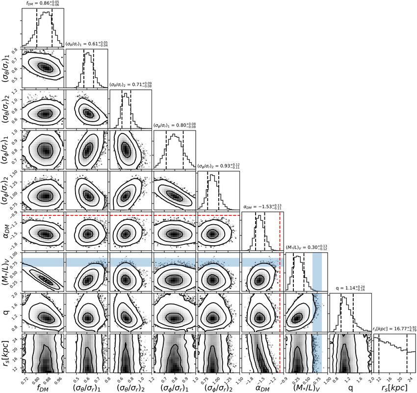
6002             M. S. Nitschai, M. Cappellari and N. Neumayer
rely on data of relatively limited quality. Moreover, these studies are   bar pattern speed, and the stellar and dark matter mass distribution
only possible for very few cases, where the full velocity information     in this region. Another work by Robin et al. (2017), investigated
is available.                                                             a wide solar neighbourhood field using the Besançon population
   For the Milky Way there have been in the past years many               synthesis model applied to RAVE and Gaia DR1 data to reproduce
surveys gathering kinematic information for stars all over the sky.       the velocities, constrain the thin and thick disc dynamical evolution
For example the Geneva–Copenhagen Survey (Nordström et al.               and determining the solar motion. In Hagen & Helmi (2018) they
2004), RAVE (Steinmetz et al. 2006), APOGEE (Allende Prieto               combine TGAS and RAVE data to study the kinematics of red clump
et al. 2008; Majewski et al. 2017), Gaia–ESO (Gilmore et al. 2012),       stars and derive the dark matter density in the solar neighbourhood.
and many others, but the Gaia mission (Gaia Collaboration et al.          They apply axisymmetric Jeans equations and get ρ DM (R , 0) =
2016) is by far the largest one, measuring billions of sources. Gaia      0.018 ± 0.002 M pc−3 . However, they also mention that the
provides us with the largest sample of three-dimensional kinematic        systematic errors are much larger and it is important to get accurate
information for stars that cover a large area on the sky.                 constrains on the stellar disc parameters.
   With this information, all these long-standing dynamical degen-           Here, we attempt to construct a first axisymmetric dynamical

                                                                                                                                                      Downloaded from https://academic.oup.com/mnras/article-abstract/494/4/6001/5825373 by guest on 31 May 2020
eracy issues disappear for the kinematics of the Milky Way from the       model of the Milky Way kinematics given by Gaia DR2. We use
Gaia mission, which are based on direct proper motion and radial          the new spherically aligned Jeans Anisotropic Method (JAMsph ;
velocities determinations for millions of individual stars: (i) one can   Cappellari 2020), which allows for general axial ratios for all three
obtain all six phase-space coordinates (three spatial coordinates and     components of the velocity ellipsoid and a spherical orientation,
three velocities), making the dimension of the observable larger than     as indicated by the Gaia data (Everall et al. 2019; Hagen et al.
that of the distribution function, thus allowing for extra parameters     2019). We want to test to what accuracy a relatively simple model
like the density to be uniquely constrained; (ii) one measures the true   can capture the richness of the Gaia kinematics. We intentionally
velocity moments, by direct summation, over many stars rather than        keep the model as simple as possible not to risk overfitting
having to infer them from integrated galaxy spectra; (iii) the stellar    kinematic features that may be due to non-equilibrium or non-
density is uniquely obtained without the need for a deprojection.         axisymmetry (e.g. bar, spiral arms, and warps) rather than tracers
   In this situation, unlike the case of every galactic dynamical         of the gravitational potential. We additionally provide a description
model for other galaxies that has been constructed in the past half a     of the mass density distribution (and circular velocity) of the Milky
century, dimensional arguments alone already imply that there is no       Way at radii r ≈ 3.6–12 kpc.
guarantee that even general models will be able to fit simultaneously        The outline of this paper is as follows: In Section 2, we briefly
all the components of the kinematics unless the model assumptions         present the Gaia DR2 data-set and introduce the Jeans model,
are sufficiently accurate. These data sets that provide full velocity     including its required components in Section 3. We present the
information then allow us to make a fundamental physical test,            resulting JAM model and the Milky Way circular velocity curve in
namely to verify whether a model based on the Newtonian equations         Section 4, before concluding in Section 5.
of motion,1 which was developed based on the motions on the scale
of the Solar system, is able to accurately predict the average motions
                                                                          2 GAIA S T E L L A R K I N E M AT I C DATA
of the stars at the scale of our Galaxy, 108 times larger.
   In recent years there has been good progress in dynamical              In 2018 April Gaia had its second data release (Gaia DR2; Gaia
modelling of the Milky Way and a summary of different dynamical           Collaboration 2018a), which contains the data collected during the
methods is given by Rix & Bovy (2013). Bovy & Rix (2013)                  first 22 months of its nominal mission lifetime. This gives for the first
used the dynamical modelling based on action integrals suggested          time a high-precision parallax and proper motion catalogue for ∼109
by Binney (2010, 2012) and Binney & McMillan (2011) where                 sources, supplemented by precise and homogeneous multiband all-
they use six-dimensional dynamical fitting with three-action-based        sky photometry and a large (a few times 106 ) radial velocity survey
distribution functions to fit abundance selected stellar populations      at the bright (G < 13) end (Gaia Collaboration 2018b).
from SEGUE. This machinery was improved and implemented in                   Some early dynamical models used subsets of the DR2 Gaia
the ROADMAPPING code (Trick, Bovy & Rix 2016), to recover the             data to infer the shape and mass of the dark matter halo (Posti &
gravitational potential by fitting an orbit distribution function to      Helmi 2019; Watkins et al. 2019; Wegg, Gerhard & Bieth 2019), the
stellar populations within the disc and it was applied to mock            Galaxy’s velocity curve (Eilers et al. 2019), or its non-equilibrium
data investigating its capabilities. The local dark matter density        features (Antoja et al. 2018). However, no study has yet attempted
was determined to be 0.0126 q−0.89 M pc−3 by Piffl et al.                to construct a comprehensive model of the bulk of the Gaia DR2,
(2014), were q is the halo’s axial ratio, using also an action based      namely the few times 106 of stars with high-quality full six-
distribution function. They investigated the vertical mass density        dimensional phase space coordinates. This is the goal of this paper.
using kinematics from giant stars in RAVE and variations in z                We use kinematics derived with Bayesian distance estimates of
from the number density determined by Jurić et al. (2008), fitting a     Schönrich, McMillan & Eyer (2019) . We assume as distance to
distribution function to the kinematics and computing the vertical        the Galactic Centre R = 8.2 kpc (Gravity Collaboration 2019),
density profile until it fits the observed profile. Kinematic models      a vertical displacement of the Sun from the mid-plane of z
based on Gaussian and Shu distribution functions were used by             = 0.02 kpc (Joshi 2007) and as solar velocities in cylindrical
Sharma et al. (2014) to constrain kinematic parameters of the Milky       Galactic coordinates (U , V , W ) = (−11.1, 247.4, 7.2) km s−1
Way using RAVE data and full phase space data from the Geneva–            (from Schönrich, Binney & Dehnen 2010; Gravity Collaboration
Copenhagen survey. Portail et al. (2017) used the made-to-measure         2019; Reid et al. 2009, respectively). The giant stars are the main
method to construct dynamical models of the bar region only, using        contribution in Gaia at distances larger than 1 kpc from the Sun and
kinematics from BRAVA, ARGOS, and OGLE and recovering the                 can be measured out to large distance due to their brightness. For
                                                                          this reason they give the most homogeneous sub-sample over the
                                                                          area we want to probe. They are selected based on their absolute
1 Relativistic   corrections are unimportant here.                        magnitude MG < 3.9, intrinsic colour (GBP − GRP )0 > 0.95 and

MNRAS 494, 6001–6011 (2020)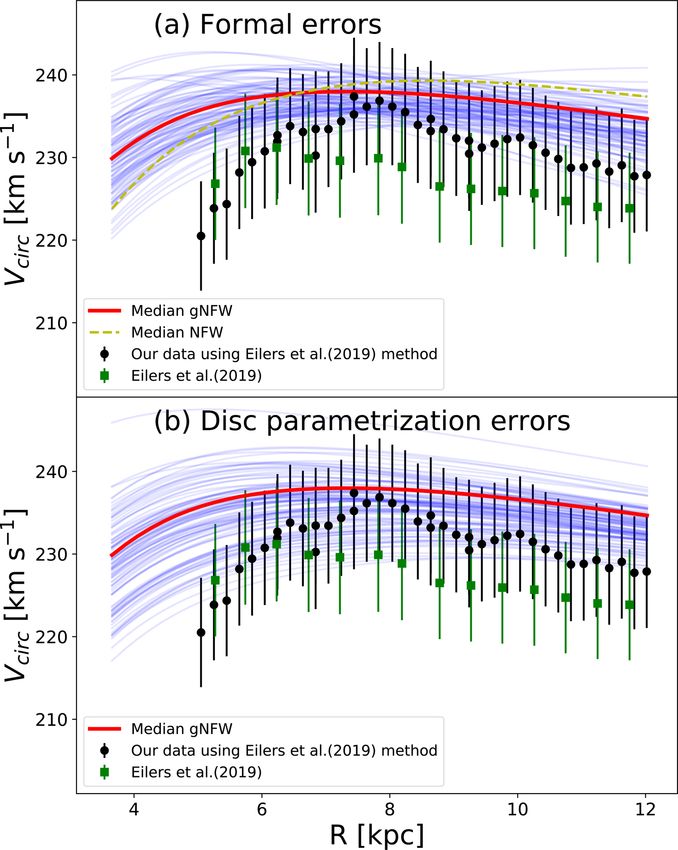
Milky Way dynamical modelling with Gaia data                        6003
positive parallaxes with relative uncertainty  /  > 5, no other             the disc area we are probing with the Gaia data and therefore we will
quality cuts were performed. This sample contains about 1.98 × 10⁶             keep it fixed for our model. Even an extreme model without a bulge
stars and covers a volume with extreme cylindrical coordinates 3.65            would not affect our conclusions. We use a bulge model of McMillan
< R < 12.02 kpc, −2.52 < z < 2.50 kpc, and −15◦ < φ < 15◦ ,                    (2017) which is an axisymmetric version of the one obtained from
which is divided into (R, z) cells of 200 × 200 pc. For each cell with         COBE/DIRBE photometry (Bissantz & Gerhard 2002)
at least 30 stars we calculated the median velocity and the velocity
                                                                                           ρ0,b             m2
dispersion. The median uncertainties over our full sub-sample are              ρb =               a exp − 2        ,                             (3)
                                                                                      (1 + m/r0 )           rcut
(vr , vφ , vz ) = (2.2, 1.3, 1.4) km s−1 , while the median velocity
error in each bin is always below 3 km s−1 , making the uncertainties          m2 = R 2 + (z/q)2 .                                                (4)
negligible for both velocity and velocity dispersion.
                                                                               We adopt the values of McMillan (2017) a = 1.8, r0 = 0.075 kpc,
                                                                               rcut = 2.1 kpc, and an axial ratio of q = 0.5. We normalize the bulge
3 METHODS                                                                      to our disc by ensuring it has the same bulge to disc ratio as the

                                                                                                                                                         Downloaded from https://academic.oup.com/mnras/article-abstract/494/4/6001/5825373 by guest on 31 May 2020
                                                                               original model (McMillan 2017), obtaining ρ 0, b = 80.81 LV pc−3 .
3.1 Model for the Milky Way stellar luminosity density                             Within 5 kpc from the Galactic Centre the bar dominates the
                                                                               kinematics (Wegg, Gerhard & Portail 2015; Bovy et al. 2019) but
The first component one needs to construct for a stellar dynamical
                                                                               since our data are mostly not covering this area we are ignoring
model is the distribution of the tracer population, from which the
                                                                               the bar in our stellar model. The small fraction of stars that might
kinematics was derived. Ideally, this would be extracted from the
                                                                               belong to the bar with radii smaller than 5 kpc should not have a
same Gaia data set we use to derive the kinematics, but this kind of
                                                                               significant effect on our model. Previous studies showed that one
model is not (yet) available.
                                                                               can measure reliable quantities outside the bar region of barred
   Therefore, we use the Milky Way stellar distribution from Jurić
                                                                               galaxies (Lablanche et al. 2012), by symmetrizing the bar density
et al. (2008) derived from the number density of main-sequence stars
                                                                               as done here.
using data from the Sloan Digital Sky Survey (SDSS). However, we
                                                                                   For use with our model, we approximate the intrinsic density of
are ignoring the stellar halo component since it is quite uncertain
                                                                               the disc + bulge stellar model with a multi-Gaussian expansion
and not as important since our data are mainly stars in the Milky
                                                                               (MGE) (Emsellem, Monnet & Bacon 1994; Cappellari 2002), by
Way disc rather than in the halo. The Jurić et al. (2008) photometric
                                                                               fitting a synthetic two-dimensional image using the MGE fitting
model was derived with data that only cover the disc plane near the
                                                                               method (Cappellari 2002) and MGEFIT software package.2 MGE
solar position and include only a smaller part of the Southern sky.
                                                                               is a general and easy way to find the potential and solve the
Hence in our work it is extrapolated to describe the whole disc area
                                                                               Jeans equations without having to modify the formalism for every
and used for giant stars rather than main-sequence stars from which
                                                                               different adopted parametrization. Most importantly, the method is
it was derived. Nevertheless, it is still the best stellar distribution
                                                                               sufficiently flexible to describe the photometry of multicomponent
we have at the moment for the disc region and probably is still a
                                                                               galaxies in great detail. Cappellari (2020) in fig. 5 presents an
good approximation for the giant stars too. In retrospect, the fact
                                                                               example of the negligible ( 1 per cent) errors one can expect in the
that our dynamical model, which has very little freedom, is able
                                                                               final Jeans kinematic predictions when approximating an analytic
to fit the data well, support the idea that the adopted stellar model
                                                                               distribution with the MGE, as we do in this paper. This indicates
may be a reasonably good representation of our tracer distribution.
                                                                               that numerical approximation errors due to the limited terms in
In fact, any change in the tracer distribution directly translates into
                                                                               the expansion should be negligible with respect to systematic
variations of the model kinematics.
                                                                               uncertainties in the data and model assumptions.
   The disc is decomposed into a sum of two exponential compo-
nents, the thin and the thick disc. This allows for different scale
lengths (Lthin , Lthick ) and heights (Hthin , Hthick ) for each component     3.2 Model for the dark matter and gas contributions

                                                        |z|
 ρD (R, z, L, H ) = ρ(R , 0) exp − R−R        L

                                                   −    H
                                                              ,         (1)    The second component of a dynamical model is the mass density of
                                                                               the Galaxy, which includes not only the stellar component but also
ρD (R, z) = ρD (R, z, Lthin , Hthin ) + f                                      the gas distribution and the dark matter halo.
              ×ρD (R, z, Lthick , Hthick ),                             (2)      We describe the dark matter as a generalized Navarro, Frenk,
                                                                               and White profile (gNFW; Wyithe, Turner & Spergel 2001), with
where ρ(R , 0) is the number density of stars in the solar neigh-
                                                                               variable inner slope α DM and axial ratio q
bourhood, and the parameter f in equation (2) is the thick disc
                                                                                           αDM
normalization relative to the thin disc. Our adopted values are the                         m          1 1 m −3−αDM
‘bias corrected’ parameters (Jurić et al. 2008): f = 0.12; (Lthin , Hthin )   ρDM = ρs                  +                ,                   (5)
                                                                                             rs        2 2 rs
= (2.6, 0.3) kpc and (Lthick , Hthick ) = (3.6, 0.9) kpc.
                                                                               with m from equation (4) and where the scale radius, rs , is also
   The parameter ρ(R , 0) was originally derived as a number
                                                                               allowed to vary between 10 and 26 kpc, consistent with values
density from star counts by Jurić et al. (2008), but since we want to
                                                                               found with the prediction of the halo mass–concentration relation
obtain meaningful stellar mass-to-light values (M∗ /L) we normalize
                                                                               M200 − c200 (Navarro, Frenk & White 1996; Klypin, Trujillo-Gomez
the density (Jurić et al. 2008) in such a way that the stellar luminosity
                                                                               & Primack 2011), for a halo mass around M200 ≈ 1.3 × 10¹² M
density at the solar radius corresponds to the local luminosity density
                                                                               (Bland-Hawthorn & Gerhard 2016), and with actual measurements
in V band ρ L = 0.056 LV pc−3 , which was derived by Flynn et al.
                                                                               for the Milky Way (e.g. Kafle et al. 2014; McMillan 2017; Eilers
(2006) using the local luminosity function and the vertical structure
                                                                               et al. 2019).
of the disc. We have chosen the V band since the SDSS data, used
to fit the disc model, and the Gaia data are including the V band.
   We further included the bulge, even though we have tested the               2 We  use the Python version 5.0.2 of the MGEFIT package available from
sensitivity of our models to it and saw that it has a minimal effect on        https://pypi.org/project/mgefit/

                                                                                                                  MNRAS 494, 6001–6011 (2020)
6004        M. S. Nitschai, M. Cappellari and N. Neumayer
    If α DM = −1, equation (5) is the classical Navaro, Frenk, and       A higher accuracy of JAMcyl with respect to Schwarzschild was
White (NFW) dark matter profile (Navarro et al. 1996). This one-         confirmed (see fig. 6 of by Jin et al. 2019) using the currently state-
dimensional profile is fitted with Gaussians using the MGE FIT 1D        of-the-art Illustris cosmological N-body simulation (Vogelsberger
procedure in the MGEFIT package (see footnote 2), and appropriately      et al. 2014). Given its spherical alignment, the JAMsph method
made oblate/prolate, for use with the model.                             should be even more accurate for the Milky Way.
    In addition, we include the gas density, even though it is quite        JAMsph is described in detail in Cappellari (2020) and here we
uncertain, again from the previous Milky Way model by McMillan           only summarize the key model assumptions. The Jeans equations
(2017). We include the mass density of both the H I and H2 gas           with the velocity ellipsoid assumed to be aligned with the spherical
in the disc of the Milky Way (equation 4 in McMillan 2017). For          coordinate system and the anisotropy defined as β = 1 − σθ2 /σr2 ,
simplicity of producing the MGE fit, we initially ignored the hole in    become (e.g. Bacon, Simien & Monnet 1983, equations 1 and 2)
the centre of this density profile, which is outside the range of our
kinematics, by removing the term in the equation that describes it,      ∂(νvr2 ) (1 + β)νvr2 − νvφ2      ∂
                                                                                 +                   = −ν    ,                                 (6)
so that the gas model only declines exponentially towards larger r.        ∂r             r               ∂r

                                                                                                                                                      Downloaded from https://academic.oup.com/mnras/article-abstract/494/4/6001/5825373 by guest on 31 May 2020
The gas density was modelled by creating an image which we fitted               ∂(νvr2 ) (1 − β)νvr2 − νvφ2           ∂
in 2-dim with the MGE FIT SECTORS routine in the MGEFIT package          (1 − β)        +                     = −ν        .                 (7)
                                                                                   ∂θ            tan θ                 ∂θ
(Cappellari 2002) as we did for the stellar model. This gas MGE
will be added to the potential density of the Milky Way but will be      These can be combined to give a linear first-order partial differential
kept fixed to the quoted mass by McMillan (2017) during the model        equation, for which standard textbook-like methods of solutions
fit, since we just want it as an estimate of the mass contribution       exist
from the gas in the disc region.                                         (1 − β) tan θ ∂(νvr2 ) 2βνvr2     ∂(νvr2 )
    Formally, removing the hole changes the force/potential inside                             −        −            = (r, θ ),               (8)
                                                                               r         ∂θ         r        ∂r
the volume we are probing and may affect our results, however, we
                                                                         where
subsequently verified that the effect is negligible by also running
a model including the central hole in the gas distribution. For                                  ∂    tan θ ∂
                                                                         (r, θ ) = v(r, θ) ×       −               .                          (9)
an accurate MGE model for the gas with the hole, we had to                                       ∂r     r ∂θ
proceed differently. We fitted equation (4) of McMillan 2017 in          A detailed solution was given by Bacon et al. (1983) and Bacon
one dimension (R) along the equatorial plane (z = 0) using the           (1985). Cappellari (2020) specialized the Jeans solution to the case
MGE FIT 1D routine in the MGEFIT package (Cappellari 2002),              where both the density and the tracer distributions are described by
while allowing for negative Gaussians (negative=True). We                the MGE parametrization and described an efficient and accurate
then described the sech2 (0.5 × z/zd ) trend in z with its best-         numerical implementation, which we used in this work.4 The use
fitting Gaussian exp(−0.195 × z2 /zd2 ), which provides an excellent     of MGE allows one to spatially vary the anisotropy by assigning
approximation. The resulting 2-dim MGE model for the gas was             different anisotropies to the various Gaussian components of the
then obtained by multiplying the 1-dim R-coordinate MGE with the         MGE.
z-Gaussian. Using this alternative 2-dim MGE gas model with a                JAMsph gives the solution of the Jeans equations for all three
hole, we found that the total density slope only change well within      mean velocity components (v r , v θ , v φ ) and the velocity dispersion
the quoted errors.                                                       in the three directions (equations 52– 54 of Cappellari 2020). We
                                                                         project the spherical velocities into cylindrical coordinates (v R , v φ ,
3.3 Bayesian JAM modelling                                               v z ). However, given that the model assumes a steady state, v R and
                                                                         v z are identically zero and do not need to be explicitly fitted. This
For the dynamical modelling we use a new solution of the axisym-         assumption is consistent with good accuracy with the Gaia maps
metric Jeans equations under the assumption of a spherically aligned     by Gaia Collaboration (2018b) which also show these velocities
velocity ellipsoid (Cappellari 2020), which was shown to describing      to be small for the purpose of this study (−15  vR  15 km s−1 ,
very accurately the dynamics of the Gaia data both in the outer halo     −10  vz  10 km s−1 ).
(Wegg et al. 2019) and the disc region (Everall et al. 2019; Hagen           The formal statistical errors in the Gaia data are quite small and
et al. 2019). This JAMsph method was developed specifically with         certainly much smaller e.g. than the actual deviations of the Milky
the Gaia data in mind. As an extreme test of the sensitivity of the      Way kinematics (or most external galaxies) from the axisymmetry
model assumption on the orientation of the velocity ellipsoid, we        and steady-state assumptions. Moreover, the Gaia data set contains
also use for comparison the cylindrically aligned JAMcyl solution        a very large number of values. In these situations, the formal
and the JAMPY package3 (Cappellari 2008).                                statistical uncertainties become meaningless as the uncertainties
   The JAMcyl method was applied to model the integral-field stellar     become entirely dominated by systematics. This is a common
kinematics of large numbers of external galaxies (see review in          issue also for the dynamical modelling of high-S/N integral-field
Cappellari 2016) and has been extensively tested against N-body          kinematics. To approximately account for systematic errors in the
simulations (Lablanche et al. 2012; Li et al. 2016) and in real          data and approximations in the model assumptions we follow the
galaxies against CO circular velocities (Leung et al. 2018), including   approach of Section 3.2 of a previous modelling paper by van den
many barred and non-perfectly-axisymmetric galaxies like the             Bosch & van de Ven (2009), as modified for Bayesian analysis in
Milky Way. In both cases, it was found to recover unbiased density       section 6.1 of Mitzkus, Cappellari & Walcher (2017). We stress
profiles, even more accurately than the more general Schwarzschild       the fact that the method is not statistically rigourous, as one should
(Schwarzschild 1979) approach (see e.g. fig. 8 of Leung et al. 2018).    expect from the fact that it tries to deal with systematic and not
                                                                         statistical uncertainties. However, it was found to work well in
3 We use the Python version 5.0.21 of the JAMPY package available from

https://pypi.org/project/jampy/                                          4 It   is included in the public JAMPY package from v6.0.

MNRAS 494, 6001–6011 (2020)
Milky Way dynamical modelling with Gaia data 6005
practice, in a number of cases. The key idea of this approximate the different components of the velocity dispersion can be directly
approach to deal with systematic uncertainties in the data is to measured from the maps, while the M∗ /L has an almost one-to-
assume that they produce a comparable contribution to the final one correspondence to the dark matter fraction fDM . The halo scale
uncertainty on the model parameters as the statistical uncertainties length rs is totally unconstrained by the Gaia data and is degenerate
in the data. This implies that, instead of adopting the standard with α DM : their combination simply defines the density total slope.
statistical confidence levels based on χ 2 (e.g. χ 2 = 1 for the While the halo axial ratio q is consistent with a spherical shape.
2
1σ uncertainty for one DOF) one should allow √ variations in the √ χ This effectively leaves to the model the freedom to vary only the
of the order of its standard deviation χ = 2(N − M) ≈ 2N ,
2
two parameters fDM and α DM , which describe the dark matter halo,
with N = 817 the number of data points fitted and M the number of to fit a set of four two-dimensional kinematic maps!
model parameters. The best-fitting standard gNFW model for the velocity maps is
In practice, we proceed as follows: First, after an initial fit, we shown in Fig. 1. We also show for comparison the model without
adopt for the kinematics a constant error of = 5.7 km s−1 , for dark matter and the best-fitting model with a ‘standard’ Navarro,
all kinematic components, to give χ 2 /DOF = 1 for the best-fitting Frenk, and White (NFW) α DM = −1 profile (Navarro et al. 1996).
Downloaded from https://academic.oup.com/mnras/article-abstract/494/4/6001/5825373 by guest on 31 May 2020
model. To include this uncertainty in the Markov chain Monte Carlo Moreover, we also show the model with free anisotropy for each
(MCMC) sampling, the error√needs to be increased in such a way of the 18 Gaussians of the MGE. The median parameters from
that a ‘misfit’ with a χ 2 = 2N using the original errors results the posterior distribution for all four models are listed in Table 1
in a fit with χ 2 = 1 with the updated, scaled errors. Hence, we together with the 1σ uncertainties, defined as half of the intervals
multiply the original error = 5.7 km s−1 by (2N)0.25 , which is enclosing 68 per cent of the posterior values, marginalized over the
√ to changing the 1σ confidence level from χ = 1 to
2
equivalent other parameters.
χ 2 = 2N . In addition, in Fig. 1 we show for reference a version of the
JAMsph or JAMcyl uses as fixed input the density of the tracer Gaia kinematic data that were symmetrized with respect to the
population (Jurić et al. 2008) and a model for the gas density equatorial plane and LOESS smoothed following Cappellari et al.
(McMillan 2017). Our standard model has nine free parameters: (i) (2015). In practice, first we use SYMMETRIZE VELFIELD8 on our
the velocity dispersion ratios or anisotropies (σ θ /σ r 5 and σ φ /σ r 6 ) for Gaia data to generate a symmetric (‘axisymmetric’) version with
both the flattest (qMGE < 0.2) Gaussian components (subscript 1) of respect to z = 0 and then we use the LOESS 2D9 routine (with
the MGE and the rest (subscript 2), to allow for some of the observed frac=0.05) of Cappellari et al. (2013b), which implements the
clear spatial variation of the anisotropy, while keeping the model as two-dimensional LOESS algorithm of Cleveland & Devlin (1988).
simple as possible. Our results are only weakly sensitive to different This gives a LOESS smoothed estimate of the kinematics at the sets
choices for separating the Gaussians with different anisotropies (see of coordinates (R, z) for the symmetrized data.
Section 4.2); (ii) the inner logarithmic slope of the gNFW profile We use the symmetrized and smoothed Gaia data as benchmark
(α DM ); (iii) the dark matter fraction fDM within a sphere of radius to quantify the quality of our JAM fits in Table 1. For this, we list the
2 2
R ; (iv) the mass-to-light ratio M∗ /LV of the stellar component in quantity χJAM /χLOESS , following Cappellari et al. (2015), for each
the V band; (v) the axial ratio q; and (vi) the scale radius (rs ) of the of the best-fitting models. This quantity has the advantage over the
dark matter profile. usual χ 2 that it approximates the χ 2 /DOF but is insensitive to the
Additionally, we also consider for comparison a model where we normalization of the kinematic uncertainties.
allow each of the 18 Gaussians in the MGE model for the stellar To partially estimate the effect on the model parameters of the
luminosity-density distribution to have a different anisotropy σ θ /σ r non equilibrium in the kinematics of the Milky Way we also fitted
and σ φ /σ r . This model has 41 free parameters. two models to two independent subsets of the Gaia data extracted
The Bayesian modelling was performed using the ADAMET7 from two azimuthal sectors (−15◦ < φ < 0◦ and 0◦ < φ < 15◦ )
package of Cappellari et al. (2013a), which implements the Adaptive of our data. The results for the two sectors (Table 1) are consistent
Metropolis algorithm by Haario, Saksman & Tamminen (2001). with each other and with the main model. As an extreme test of the
This is used to estimate the posterior distribution, as in standard sensitivity of our model to the assumptions on the orientation of the
MCMC methods (Gelman et al. 2013), to get the confidence levels velocity ellipsoid, we also have fit a model (JAMcyl ) that assumes
of the best-fitting parameters and to show the relations between the a cylindrically aligned velocity ellipsoid (Cappellari 2008). The
different parameters. We adopted constant priors on all parameters, JAMsph model gives a slightly better fit to the data than JAMcyl ,
in such a way that the probability of the model, given the data, is consistently with the finding that the Milky Way velocity ellipsoid
just proportional to the likelihood P (data|model) ∝ exp (− χ 2 /2). is nearly spherical aligned (Everall et al. 2019; Hagen et al. 2019).
However, the difference between the parameters inferred by two,
JAMsph and JAMcyl , models is minimal (Table 1) as the two solutions
4 R E S U LT S are not very different in the disc plane.
Three results can be inferred from Fig. 1: (i) The most striking
4.1 JAM fit to the Gaia data and important is how well this simple equilibrium model is able to
Formally, our standard model has nine free parameters, however, capture the average Gaia kinematics. Here, the main model residuals
most of them are either directly constrained by the data or irrelevant appear due to the known 15 per cent non-equilibrium and non-
and marginalized over. We include these 9 parameters just not to risk axisymmetry features (Gaia Collaboration 2018b), which cannot
underestimating the model uncertainties. The four ratios between be described by an equilibrium model. In fact, most of the model
5 ForJAMcyl this is σ z /σ R . 8 This routine is included in the PLOTBIN package available from https:
6 ForJAMcyl this is σ φ /σ R . //pypi.org/project/plotbin/
7 We use the Python version 2.0.7 of the ADAMET package available from 9 We use the Python version 2.0.11 of the LOESS package available from
https://pypi.org/project/adamet/ https://pypi.org/project/loess/
MNRAS 494, 6001–6011 (2020)6006 M. S. Nitschai, M. Cappellari and N. Neumayer
Downloaded from https://academic.oup.com/mnras/article-abstract/494/4/6001/5825373 by guest on 31 May 2020
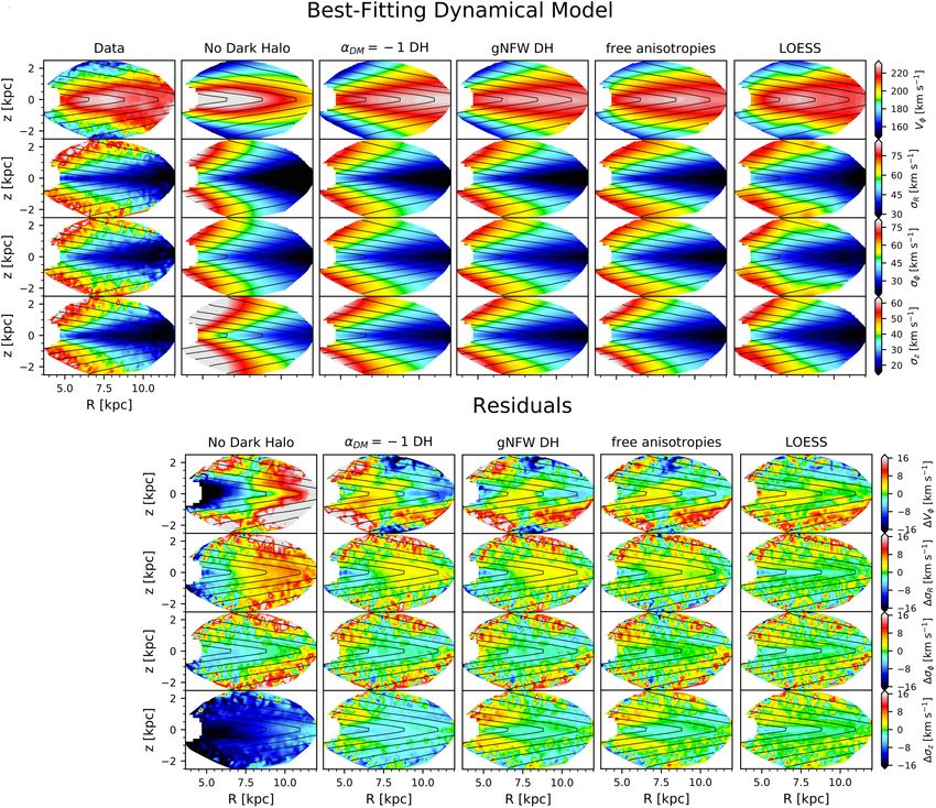
Figure 1. Data versus models. From left to right: (i) Gaia data, (ii) the best-fitting JAMsph model without dark matter, (iii) the best model with a ‘standard’
Navarro, Frenk, and White (NFW) dark matter profile, (iv) the best-fitting model with gNFW halo profile, with free inner logarithmic slope, and two free
anisotropies (see text), (v) the best-fitting model with a different anisotropy for each MGE Gaussian, and (vi) a symmetrized and LOESS-smoothed version
of the Gaia data. The latter is shown for reference and, given that it makes no other assumption than symmetry and small-scale smoothness, it essentially
represents the best fit that one can expect with any axisymmetric model. Below each model there are the corresponding residuals (data − model). From top to
bottom the rows show the mean azimuthal velocity (v φ ), the velocity dispersion in radial (σ R ), azimuthal (σ φ ), and vertical (σ z ) direction in Galactic cylindrical
coordinates.
residuals seem associated with the spiral-wave pattern visible in the one, with our median dark halo slope α DM = −1.53 ± 0.12. In
face-on view of the kinematics of the Milky Way disc in fig. 10 particular, an NFW halo systematically overestimates σ z and the
of Gaia Collaboration (2018b). The fact that most of the residuals radial gradient in v φ . The halo slope lies in the range expected from
are due to non-axisymmetry is also clearly visible by comparing simple predictions for halo contractions (Gnedin et al. 2004) for
the residuals of the best-fitting model to those of the symmetrized samples of real galaxies (e.g. fig. 2 in Cappellari et al. 2013a). This
data (Fig. 1): the largest JAM residuals are in the Vφ components, is consistent with previous work indicating a steeper slope than the
but most of those also stand out with respect to the symmetrized standard NFW is needed in the disc region of the Milky Way around
Gaia data. The same is true for the major deviations in the JAM fits the solar region (Cole & Binney 2017; Portail et al. 2017).
to the other components. This good agreement is further quantified The anisotropies of the data and model are in approximate
2 2
by the χJAM /χLOESS ratio in Table 1, which shows values quite agreement, although the model is by construction smoother than the
close to one, especially when allowing for ‘free anisotropies’. (ii) data and does not try to reproduce the sharp anisotropy variations
It is clear that a model without dark matter completely fails to and asymmetries. These are unlikely to contain information on the
describe the observations, (iii) moreover, a standard NFW dark gravitational potential, but are instead due to non-equilibrium and
matter profile does not provide an equally good fit as the best-fitting non-axisymmetry. With a more general model like Schwarzschild
MNRAS 494, 6001–6011 (2020)Milky Way dynamical modelling with Gaia data 6007
Table 1. Median parameters and 68 per cent (1σ ) confidence intervals for the spherically or cylindrically aligned JAM models and the χ 2 values for the
best-fitting models.
Parameter Spherically aligned JAMsph Cylindrically aligned
JAMcyl
No dark halo NFW dark halo gNFW dark halo −15◦ < φ < 0◦ 0◦ < φ < 15◦ Free anisotropies gNFW dark halo
(1) α DM − −1 − 1.53 ± 0.12 − 1.52 ± 0.13 − 1.50 ± 0.12 − 1.54 ± 0.14 − 1.48 ± 0.13
(2) fDM − 0.73 ± 0.05 0.86 ± 0.06 0.85 ± 0.06 0.84 ± 0.05 0.90 ± 0.06 0.91 ± 0.05
(3) rs [kpc] − 10.8 ± 1.0 16.8 ± 5.4 17.2 ± 5.3 17.1 ± 5.4 17.6 ± 4.9 16.2 ± 5.2
(4) qDM − 1.16 ± 0.25 1.14 ± 0.21 1.12 ± 0.23 1.33 ± 0.31 1.03 ± 0.22 1.40 ± 0.35
(5) (σ θ /σ r )1 0.97 ± 0.14 0.67 ± 0.05 0.62 ± 0.05 0.61 ± 0.05 0.60 ± 0.05 − 0.63 ± 0.04a
(6) (σ θ /σ r )2 0.82 ± 0.11 0.75 ± 0.08 0.71 ± 0.09 0.76 ± 0.10 0.73 ± 0.11 − 0.83 ± 0.06a
(7) (σ φ /σ r )1 0.87 ± 0.20 0.79 ± 0.08 0.80 ± 0.08 0.78 ± 0.09 0.77 ± 0.08 − 0.80 ± 0.07b
Downloaded from https://academic.oup.com/mnras/article-abstract/494/4/6001/5825373 by guest on 31 May 2020
(8) (σ φ /σ r )2 0.87 ± 0.20 0.94 ± 0.12 0.93 ± 0.12 0.95 ± 0.15 0.97 ± 0.14 − 0.96 ± 0.13b
(9) (M∗ /L)V 1.82 ± 0.03 0.58 ± 0.12 0.30 ± 0.13 0.34 ± 0.13 0.38 ± 0.13 0.21 ± 0.14 0.26 ± 0.12
(10) χ 2 10611 3672 3251 3078 2816 2698 3460
2 2
(11) χJAM /χLOESS 4.82 1.67 1.48 1.41 1.44 1.23 1.57
(12) (χJAM /χLOESS )2Vφ 6.39 2.37 1.98 1.91 1.89 1.38 2.06
(13) (χJAM /χLOESS )2σR 2.52 1.29 1.22 1.20 1.32 1.14 1.30
(14) (χJAM /χLOESS )2σφ 1.61 1.21 1.29 1.11 1.22 1.12 1.20
(15) (χJAM /χLOESS )2σz 14.03 1.87 1.47 1.32 1.49 1.27 1.87
Note. Row (1): the inner logarithmic slope of the gNFW profile; Row (2): the dark matter fraction within a sphere of radius R = 8.2 kpc; Row (3): the scale radius, and
Row (4): the axial ratio of the gNFW. Row (5) and (6): the velocity dispersion ratio (σ θ /σ r )1 and (σ θ /σ r )2 . Similar row (7) and (8): the velocity dispersion ratio (σ φ /σ r )1
2
and (σ φ /σ r )2 . Row (9): the mass-to-light ratio. Row (10): the χ 2 of the best-fitting models and row (11): quality of the best-fitting models, with χJAM measured from the
2
JAM models and χLOESS from the symmetrized data. Row (12), (13), (14), and (15): the quality of the best-fitting models for each individual velocity component (v φ , σ R ,
σ φ , σ z ). a See footnote 5. b See footnote 6.
(1979) method one could fit every detail of the data, down to The total-density distribution is the quantity that the dynamical
the noise. However, a better fit will not necessarily constitute models directly measure. This is very tightly constrained by the
an improvement in the recovered density, because there is a risk Gaia data and it is shown in Fig. 3. From the posterior of the
of interpreting non-equilibrium or non-axisymmetry features as models we measure a total density mean logarithmic slope of
tracers of an axisymmetric equilibrium model. Tests on real galaxies α tot ≡ log ρ tot /log r = −2.149 ± 0.055 in the radial range
(Leung et al. 2018) and simulations (Jin et al. 2019) indicate that 3.6–12 kpc of the data. These radii correspond to about 0.9–2.9
Schwarzschild models provides a less accurate recovery of the true half-light radii Remax , for our measured10 Remax ≈ 4.122 kpc. The
density than JAM in this situation. Thus, we intentionally kept the measured total-density slope is consistent with the ‘universal’ slope
standard model simple, not to risk over-interpreting features in the α tot ≈ −2.19 ± 0.03 inferred at comparable radii on early-type disc
data that are not real or not tracer of an equilibrium potential. galaxies (Cappellari et al. 2015) with effective velocity dispersion
Our model has a total density at the solar position of ρ tot (R ) = not smaller than the Milky Way’s value (Kormendy & Ho 2013) σ e
0.0640 ± 0.0043 M pc−3 and a dark matter density of ρ DM (R ) = 105 ± 20 km s−1 .
= 0.0115 ± 0.0020 M pc−3 , corresponding to a dark matter We also investigate how much the uncertainties of the
energy density of 0.437 ± 0.076 GeV cm−3 where the uncertainties parametrization of the Milky Way stellar tracer distribution affect
include systematics and are not purely statistical. These values are our JAMsph results. For this, we vary the disc parameters of Jurić
broadly consistent with previous determinations (McKee, Parravano et al. (2008) within the quoted errors and then redo the JAMsph fit
& Hollenbach 2015; McMillan 2017). using the CAPFIT least-squares program.11 This is repeated for 100
The posterior distribution of the parameters for the gNFW model different disc models, for random values of the scale heights, scale
are shown in Fig. 2. This figure also shows the expected covariance lengths, and the fraction of the thick disc normalization, within the
between the mass-to-light ratio, the dark matter fraction, and the given 20 per cent 1σ uncertainties (Jurić et al. 2008). The result
inner slope of the halo: models with steeper (more negative) α DM for the total density can be seen in panel (b) of Fig. 3. Here, the
have lower (M∗ /L)V ratio and higher dark matter fraction fDM . This blue lines indicate the systematic error due to the Milky Way stellar
distribution also shows that an NFW profile (red-dashed line in tracer model. This gives us an alternative estimate of the value and a
Fig. 2) is outside the 3σ confidence level. In addition, as comparison systematic error α tot ≡ log ρ tot /log r = −2.194 ± 0.044 and the
the blue-shaded region indicates the stellar mass-to-light ratio from logarithmic slope of the gNFW profile is α DM = −1.455 ± 0.055,
stellar counts 0.75 M /LV (15 per cent uncertainty at 1σ level from which is comparable to the previous estimate.
Flynn et al. 2006). This shows that our model (M∗ /L)V is consistent During this testing of these systematic errors, we saw that higher
with the stellar-counts determination within the errors. Our model values for the scale height and length of our disc models seem to
strongly excludes flattened haloes and favours a nearly round one, give JAM models that agree even better with our data. We leave
consistent with recent Gaia results (Wegg et al. 2019). further exploration of this aspect to a subsequent study.
4.2 Total density profile
Having found our best-fitting model we can find the total density 10 Using MGE HALF LIGHT ISOPHOTE in the JAMPY package.
profile, using the MGE RADIAL DENSITY procedure in the JAMPY 11 This is part of the Python package PPXF by Cappellari (2017) available
package (see footnote 3). here https://pypi.org/project/ppxf/
MNRAS 494, 6001–6011 (2020)6008 M. S. Nitschai, M. Cappellari and N. Neumayer
Downloaded from https://academic.oup.com/mnras/article-abstract/494/4/6001/5825373 by guest on 31 May 2020
Figure 2. gNFW parameters corner plot. Each panel shows the posterior probability distribution marginalized over two dimensions (contours) and one
dimension (histograms). The parameters are (i) the dark matter fraction fDM inside a sphere of radius R = 8.2 kpc; (ii) the velocity dispersion ratios [(σ θ /σ r )1 ,
(σ φ /σ r )1 ] of the Gaussians flatter than qMGE = b/a = 0.2, and the rest [(σ θ /σ r )2 , (σ φ /σ r )2 ]; (iii) the inner dark matter halo logarithmic slope α DM ; (iv) the
stellar mass-to-light ratio (M∗ /L)V ; (v) the axial ratio q of the dark matter halo; and (vi) the scale radius rs for the dark matter halo. The thick contours represent
the 1σ , 2σ and 3σ confidence levels for one degree of freedom. The red dashed line marks the ‘standard’ α DM = −1 slope of the NFW (Navarro et al. 1996)
dark matter profile and the blue shaded band indicates a mass-to-light ratio estimate from stellar counts (Flynn et al. 2006). The numbers with errors on top of
each plot are the median (black dashed lines) and 16th and 84th percentiles of the posterior for each parameter, marginalized over the other parameters.
Our model results depend on some arbitrary choices, like the possible anisotropies, separated both in radius (smaller or larger
number of Gaussians used in the MGE fit, and the axial ratio qMGE than one effective radii) and flattening at qMGE = 0.3 (instead of
at which we separate Gaussians with different anisotropies. We our standard qMGE = 0.2) we get α tot = −2.075. So even with
tested the sensitivity of the most robust quantity from the model, this different choice to separate the anisotropies, the result is still
the total density slope, to these choices. If we force the MGE fit consistent at the level of the quoted errors.
to have 35 Gaussians, instead of the 18 of our standard model, and
perform a least-squares fit, we obtain a slope for the total density of
α tot = −2.203, which agrees within the quoted errors with the least- 4.3 Circular velocity curve
squares fit for our standard model which has α tot = −2.185 (this is Having found a model that describes our Gaia data we can also
slightly different from the median value from the model posterior derive the circular velocity, using the MGE VCIRC procedure in the
quoted previously in this Section). Additionally, if we allow four JAMPY package (see footnote 3).
MNRAS 494, 6001–6011 (2020)Milky Way dynamical modelling with Gaia data 6009
Downloaded from https://academic.oup.com/mnras/article-abstract/494/4/6001/5825373 by guest on 31 May 2020
Figure 3. Milky Way total density profile. (a) The blue shaded region shows
100 realizations of the density profile from the model posterior of Fig. 2.
The black line is the median density for the NFW α DM = −1 model. (b)
Density profiles obtained by randomly varying the assumed parametrization
for the stellar disc (Jurić et al. 2008) within the quoted errors and re-running Figure 4. Circular velocity for the model. The red line is the circular
the whole model fitting procedure. velocity of our median gNFW model, the green squares are the recent
measurements of Eilers et al. (2019), the black points are derived with a
subset of our data, restricting them to the equatorial plane and the Eilers
The circular velocity of the Milky Way disc region is plotted et al. (2019) method and the yellow dashed line is for the mean normal NFW
as a red line for the gNFW and as a dashed yellow line for the profile. The blue lines in panel (a) are the circular velocities of 100 random
normal NFW profile in panel (a) of Fig. 4. The black points are parameters of the posterior distribution that give the formal error from the fit
derived with a subset (|z| < 0.5 kpc or tan (z/R) < 6◦ ) from our and in panel (b) they are 100 different disc models that give the systematic
data when using the same non-parametric method of Eilers et al. error due to disc parametrization.
(2019), also based on the axisymmetric Jeans equations, to calculate
the circular velocity and the green squares are the measurements kinematic errors. At the solar position we get a value of v circ (R )
of Eilers et al. (2019). The small offset between our values and the = 236.5 ± 1.8 km s−1 . This value also agrees well with the value
previous work by Eilers et al. (2019) is coming from our slightly of Eilers et al. (2019) (229.0 ± 0.2 km s−1 ), where they use a quite
higher value of the solar velocity because of the newest Gravity different stellar sample, stellar distance estimates, and modelling
Collaboration (2019) results for the distance to the Galactic Centre. assumptions, and with another recent work by Mróz et al. (2019)
The difference between our values using the method of Eilers et al. (233.6 ± 2.8 km s−1 ) in which they construct the rotation curve of
(2019) (black dots) and our result from the JAMsph model (red line) the Milky Way using the proper motion and radial velocities from
is expected, since the data used for Eilers et al. (2019) method are Gaia for classical Cepheids.
only covering the equatorial plane of the Galaxy (|z| < 0.5 kpc The result for the effect of the uncertainties of the parametrization
or tan (z/R) < 6◦ ) while for our model all the data reaching up of the Milky Way stellar tracer distribution on the circular velocity
to 2.5 kpc in z-direction were used. Moreover, also the different can be seen in panel (b) of Fig. 4. Here, the blue lines indicate the
parametrization of the tracer distribution in Eilers et al. (2019) systematic error due to the Milky Way stellar tracer model. This
method and our makes a difference. We have investigated this further gives us an alternative estimate of the value and systematic error
and can reproduce almost exactly their circular velocity curve if v circ (R ) = 236.3 ± 3.1 km s−1 , which is comparable to the previous
we use the same kinematics and the same tracer distribution of estimate.
Pouliasis, Di Matteo & Haywood (2017) with a spherical (qDM = 1)
NFW dark matter halo (Nitschai et al., in preparation). Reassuringly,
5 CONCLUSION
the two circular velocities are consistent within the estimated quite
small systematic uncertainties. The model with NFW halo would The model presented is the first stringent test of the Newtonian
produce an inconsistent circular velocity, supporting the finding that equations of motion on galactic scales. It demonstrates that we
this is excluded by the Gaia data. already have a remarkably accurate knowledge of the mass distri-
The blue transparent lines are 100 random realizations for the bution in our Milky Way and we can concisely describe the main
circular velocity from the posterior distribution that indicates the average characteristics of the observed stellar kinematics with a
formal uncertainty for our mean circular velocity but include minimal set of assumptions. The model also shows that the average
our approximate treatment for systematics by scaling the input kinematics of the Milky Way, outside of the bar region, can be
MNRAS 494, 6001–6011 (2020)6010 M. S. Nitschai, M. Cappellari and N. Neumayer
well described by an axisymmetric and equilibrium model. The Cappellari M., 2020, MNRAS, 494, 4819
fact that we can well describe the Galactic kinematics, regardless Cappellari M. et al., 2006, MNRAS, 366, 1126
of relatively minor deviations from equilibrium and axisymmetry Cappellari M. et al., 2013a, MNRAS, 432, 1709
(Widrow et al. 2012; Antoja et al. 2018; Gaia Collaboration 2018b), Cappellari M. et al., 2013b, MNRAS, 432, 1862
Cappellari M. et al., 2015, ApJ, 804, L21
is consistent with observations of external galaxies, where such
Cleveland W. S., Devlin S. J., 1988, J. Am. Stat. Assoc., 83, 596
deviations are widespread, but models can still capture the average
Cole D. R., Binney J., 2017, MNRAS, 465, 798
kinematic properties (Cappellari et al. 2013a) and recover circular Courteau S. et al., 2014, Rev. Mod. Phys., 86, 47
velocity profiles to 10 per cent accuracy (Leung et al. 2018), even de Lorenzi F. et al., 2009, MNRAS, 395, 76
from data of much inferior quality. Eilers A.-C., Hogg D. W., Rix H.-W., Ness M. K., 2019, ApJ, 871, 120
The Gaia data are going to improve in accuracy with subsequent Emsellem E., Monnet G., Bacon R., 1994, A&A, 285, 723
data releases. Moreover, when not relying entirely on parallactic Everall A., Evans N. W., Belokurov V., Schönrich R., 2019, MNRAS, 489,
distances, one can significantly increase the extent of the region 910
where kinematics can be measured (Wegg et al. 2019). Dynamical Flynn C., Holmberg J., Portinari L., Fuchs B., Jahreiß H., 2006, MNRAS,
Downloaded from https://academic.oup.com/mnras/article-abstract/494/4/6001/5825373 by guest on 31 May 2020
models will soon be able to study our Galaxy’s density distribution 372, 1149
Gaia Collaboration, 2016, A&A, 595, A1
over larger distances. These models are starting to provide a
Gaia Collaboration, 2018a, A&A, 616, A1
description of the dynamics of the Milky Way at a level that is
Gaia Collaboration, 2018b, A&A, 616, A11
impossible to achieve in external galaxies. This is providing a Gebhardt K. et al., 2000, AJ, 119, 1157
key benchmark for our knowledge of galactic dynamics that will Gelman A., Carlin J., Stern H., Dunson D., Vehtari A., Rubin D., 2013,
complement much less detailed studies of much larger samples of Bayesian Data Analysis, Third Edition. Chapman & Hall, Taylor &
external galaxies. Francis
The kinematics used in this paper and the MGE components can Gerhard O. E., 1993, MNRAS, 265, 213
be found as Supplementary data in the online version. Gilmore G. et al., 2012, The Messenger, 147, 25
Gnedin O. Y., Kravtsov A. V., Klypin A. A., Nagai D., 2004, ApJ, 616, 16
Gravity Collaboration, 2019, A&A, 625, L10
AC K N OW L E D G E M E N T S Haario H., Saksman E., Tamminen J., 2001, Bernoulli, 7, 223
Hagen J. H. J., Helmi A., 2018, A&A, 615, A99
M.S. Nitschai warmly thanks the two scholarships, Deutscher Hagen J. H. J., Helmi A., de Zeeuw P. T., Posti L., 2019, A&A, 629,
Akademischer Austauschdienst (German Academic Exchange Ser- A70
vice) - Programm zur Steigerung der Mobilität von Studieren- Jin Y., Zhu L., Long R. J., Mao S., Xu D., Li H., van de Ven G., 2019,
den deutscher Hochschulen (‘DAAD-PROMOS-Stipendium’) and MNRAS, 486, 4753
‘Baden-Württemberg-STIPENDIUM’, for the financial support Joshi Y. C., 2007, MNRAS, 378, 768
during the stay abroad working on this project and the Astrophysics Jurić M. et al., 2008, ApJ, 673, 864
Kafle P. R., Sharma S., Lewis G. F., Bland-Hawthorn J., 2014, ApJ, 794, 59
sub-department of the University of Oxford for the hospitality
Klypin A. A., Trujillo-Gomez S., Primack J., 2011, ApJ, 740, 102
during that time. NN gratefully acknowledges support by the
Kormendy J., Ho L. C., 2013, ARA&A, 51, 511
Deutsche Forschungsgemeinschaft (DFG, German Research Foun- Krajnović D., Cappellari M., Emsellem E., McDermid R. M., de Zeeuw P.
dation) – Project-ID 138713538 – SFB 881 (‘The Milky Way T., 2005, MNRAS, 357, 1113
System’, subproject B8). This work has made use of data from Lablanche P.-Y. et al., 2012, MNRAS, 424, 1495
the European Space Agency (ESA) mission Gaia (https://www. Leung G. Y. C. et al., 2018, MNRAS, 477, 254
cosmos.esa.int/gaia), processed by the Gaia Data Processing and Li H., Li R., Mao S., Xu D., Long R. J., Emsellem E., 2016, MNRAS, 455,
Analysis Consortium (DPAC, https://www.cosmos.esa.int/web/gai 3680
a/dpac/consortium). Funding for the DPAC has been provided by Majewski S. R. et al., 2017, AJ, 154, 94
national institutions, in particular the institutions participating in McKee C. F., Parravano A., Hollenbach D. J., 2015, ApJ, 814, 13
McMillan P. J., 2017, MNRAS, 465, 76
the Gaia Multilateral Agreement.
Mitzkus M., Cappellari M., Walcher C. J., 2017, MNRAS, 464, 4789
Mróz P. et al., 2019, ApJ, 870, L10
Navarro J. F., Frenk C. S., White S. D. M., 1996, ApJ, 462, 563
REFERENCES
Nordström B. et al., 2004, A&A, 418, 989
Allende Prieto C. et al., 2008, Astron. Nachr., 329, 1018 Piffl T. et al., 2014, MNRAS, 445, 3133
Antoja T. et al., 2018, Nature, 561, 360 Portail M., Gerhard O., Wegg C., Ness M., 2017, MNRAS, 465, 1621
Bacon R., 1985, A&A, 143, 84 Posti L., Helmi A., 2019, A&A, 621, A56
Bacon R., Simien F., Monnet G., 1983, A&A, 128, 405 Pouliasis E., Di Matteo P., Haywood M., 2017, A&A, 598, A66
Bender R., 1990, A&A, 229, 441 Reid M. J. et al., 2009, ApJ, 700, 137
Binney J., 2010, MNRAS, 401, 2318 Rix H.-W., Bovy J., 2013, A&A Rev., 21, 61
Binney J., 2012, MNRAS, 426, 1328 Rix H.-W., de Zeeuw P. T., Cretton N., van der Marel R. P., Carollo C. M.,
Binney J., Mamon G. A., 1982, MNRAS, 200, 361 1997, ApJ, 488, 702
Binney J., McMillan P., 2011, MNRAS, 413, 1889 Robin A. C., Bienaymé O., Fernández-Trincado J. G., Reylé C., 2017, A&A,
Bissantz N., Gerhard O., 2002, MNRAS, 330, 591 605, A1
Bland-Hawthorn J., Gerhard O., 2016, ARA&A, 54, 529 Rybicki G. B., 1987, in de Zeeuw P. T., ed., Proc. IAU Symp. 127, Structure
Bovy J., Rix H.-W., 2013, ApJ, 779, 115 and Dynamics of Elliptical Galaxies. Kluwer, Dordrecht, p. 397
Bovy J., Leung H. W., Hunt J. A. S., Mackereth J. T., Garcı́a-Hernández D. Schönrich R., Binney J., Dehnen W., 2010, MNRAS, 403, 1829
A., Roman-Lopes A., 2019, MNRAS, 490, 4740 Schönrich R., McMillan P., Eyer L., 2019, MNRAS, 487, 3568
Cappellari M., 2002, MNRAS, 333, 400 Schwarzschild M., 1979, ApJ, 232, 236
Cappellari M., 2008, MNRAS, 390, 71 Sharma S. et al., 2014, ApJ, 793, 51
Cappellari M., 2016, ARA&A, 54, 597 Steinmetz M. et al., 2006, AJ, 132, 1645
Cappellari M., 2017, MNRAS, 466, 798 Trick W. H., Bovy J., Rix H.-W., 2016, ApJ, 830, 97
MNRAS 494, 6001–6011 (2020)You can also read