EXPERIMENTAL WEEKLY TO SEASONAL U.S. FORECASTS WITH THE REGIONAL SPECTRAL MODEL
←
→
Page content transcription
If your browser does not render page correctly, please read the page content below
EXPERIMENTAL WEEKLY TO
              SEASONAL U.S. FORECASTS
                WITH THE REGIONAL
                  SPECTRAL MODEL
                                                              BY    J. ROADS

                 Since 1997, the Scripps Experimental Climate Prediction Center (ECPC) has been
                 routinely making near-real-time experimental global and regional dynamical weekly
                            to seasonal forecasts of many pertinent geophysical variables.

     A
            s described previously Roads et al. 2001a, here-           tional analysis, which is available to interested research-
            after RCF), the Scripps Experimental Climate               ers, almost without fail, every day in near–real time on
            Prediction Center (ECPC) has been making rou-              NCEP rotating disk archives. Transforming NCEP’s
     tine, near-real-time, long-range experimental global              higher-resolution operational global analyses to lower
     and regional dynamical forecasts since 27 September               (vertical and horizontal) resolution initial conditions for
     1997. The global spectral model (GSM) used for these              the GSM, 7-day global forecasts are made every day,
     forecasts is that of National Centers for Environmen-             and every weekend these GSM forecasts are extended
     tal Prediction’s (NCEP; Kalnay et al. 1996; see also              to 16 weeks. RCF (see also Roads et al. 2001b; Chen
     Roads et al. 1999) used for the NCEP–National Center              et al. 2001; Roads and Brenner 2002; Roads and Chen
     for Atmospheric Research (NCAR) reanalysis. The                   2003) provided a preliminary evaluation of the
     initial conditions and SST boundary conditions for these          12-week forecast capability of the GSM for many re-
     experimental GSM forecasts come from the NCEP                     gions for the first 2 yr and indicated that there were
     Global Data Assimilation (GDAS) 0000 UTC opera-                   places and times when the GSM 12-week forecasts of
                                                                       many relevant geophysical variables were skillful.
                                                                           Utilizing these GSM forecasts as lateral boundary
AFFILIATIONS:    ROADS—Scripps Experimental Climate Prediction         conditions, the ECPC also routinely makes higher-
Center, University of California, San Diego, La Jolla, California
                                                                       resolution regional spectral model (RSM; Juang and
CORRESPONDING AUTHOR: J. Roads, Scripps Experimental
Climate Prediction Center, UCSD, 0224, La Jolla, CA
                                                                       Kanamitsu 1994; Juang et al. 1997) forecasts for vari-
92093-0224                                                             ous regions (United States, the Southwest, California,
E-mail: jroads@ucsd.edu                                                Brazil). Several papers have described the RSM re-
DOI: 10.1175/BAMS-85-12-1887                                           gional simulation capability (Chen et al. 1999; Ander-
                                                                       son et al. 2000a,b, 2001; Anderson and Roads 2002; Han
In final form 14 May 2004
©2004 American Meteorological Society                                  and Roads 2004; Roads and Chen 2000; Roads et al.
                                                                       2003a,b,c; Takle et al. 1999). These papers have shown

     AMERICAN METEOROLOGICAL SOCIETY                                                                     DECEMBER 2004           | 1887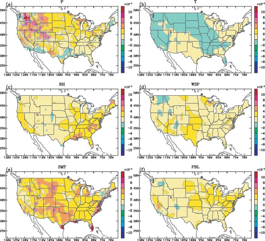
that the RSM is certainly useful for simulating and            the global and regional forecasts that may be especially
     understanding regional climates. The RSM, like other           relevant to various hydrology, fire danger, and atmo-
     regional models, provides increased focus for specific         spheric pollution communities. Accurate forecasts of
     regions, can be more constrained by realistic large-scale      precipitation, temperature (2 m), and soil moisture
     conditions, and can make use of higher-resolution re-          would be useful to the hydrologic community; precipi-
     gional datasets for validation.                                tation, temperature (2 m), relative humidity (2 m), and
        However, except for a few notable cases (e.g.,              wind speed to the fire community; and wind speed
     Anderson et al. 2000a,b, 2001; Leung et al. 2003) the          (10 m) and planetary boundary layer height to the air
     RSM has not yet unambiguously indicated that it pro-           pollution community. This ability to provide a diverse
     vides a better regional simulation capability than the         set of consistent geophysical outputs is one of the rea-
     bounding global analyses. This has been somewhat               sons that dynamical models are potentially more use-
     surprising, since it is commonly assumed that the              ful than statistical forecasting methodologies, which
     interactions of a regional model with its associated           focus in on only one or two variables, such as, for in-
     higher-resolution landscape should provide better re-          stance, temperature and precipitation, which must
     gional simulations and predictions. We do already              have adequate observational data.
     know that increased resolution alone is not sufficient             The next section provides an overview of our meth-
     to achieve better global simulations. In global models,        odology (models, observations, error measures), fol-
     physical parameterization improvements are some-               lowed by an examination of geographic, temporal, and
     times much more important (see, e.g., Marshall et al.          forecast lag characteristics of the experimental regional
     1997). Also, increased skill of regional models can some-      forecasts. The article concludes with a summary of the
     times be more easily attributed to regional model              evaluations. In short, our current regional forecasts
     physical parameterization improvements than to in-             have significant skill, but this forecast skill is not sig-
     creased resolution (see, e.g., Chen 2002; Roads et al.         nificantly better than that obtained from the driving
     2003a; Han and Roads 2004). In addition to further             GSM.
     improving the RSM parameterizations, we are now
     beginning to understand that if the regional simula-           METHODOLOGY. GSM forecasts. The GSM fore-
     tions are to be significantly better than the bounding         casts used for this study were previously described in
     global analysis, then additional regional observations         many papers (e.g., RCF; Roads 2004). Again, the
     will probably have to be included. For example, the            GSM is based upon the medium-range forecast (MRF)
     pending regional reanalysis (Mesinger et al. 2002) makes       model used for the NCEP–NCAR reanalyses (Kalnay
     use of regional precipitation and other observations,          et al. 1996; Kanamitsu et al. 2002). The GSM has a tri-
     along with improved land surface and other param-              angular truncation of T62 (192 ¥ 94 global Gaussian
     eterizations, in order to develop an improved regional         grid) and 18 irregularly spaced vertical levels (18LT62).
     analysis.                                                      Seven-day GSM forecasts, initialized every day from
        What about long-range forecasts with regional               the 0000 UTC NCEP GDAS operational analysis,
     models? Do regional models in general and our ver-             and 16-week GSM forecasts made every weekend pro-
     sion of the RSM in particular make useful regional fore-       vide the basic large-scale driving data for the RSM.
     casts when bounded by global forecasts instead of glo-         During the weekly 16-week (and also daily 7-day) fore-
     bal analyses? This question is especially important            casts, it is assumed that the initial SST anomaly is
     when considering global change projections that need           constant (persistent). The GDAS initial conditions
     to be downscaled for regional applications (see, e.g.,         have been accessed almost every day from 0000 UTC
     Chen et al. 2003; Han and Roads 2004), but also is rel-        27 September 1997 to the present (28LT126 NCEP glo-
     evant to current seasonal global forecasts. Roads et al.       bal analyses were available from 0000 UTC 27 Sep-
     (2004) and Roads (2004) examined the seasonal fore-            tember 1997 to 1800 UTC 14 March 2000; 42LT170
     cast capability of fire danger and precipitation and           were available from 0000 UTC 15 March 2000 to 1800
     found that the RSM was perfectly capable of providing          UTC 14 July 2002; 62LT256 became available 0000 UTC
     significant forecast skill at weekly to seasonal time scales   15 July 2002). These higher-resolution analyses are
     for many U.S. regions, but for at least the case of pre-       transformed to lower-resolution initial conditions
     cipitation forecasts, it was not clear that the regional       (18LT62) by linearly interpolating between vertical
     forecast skill was significantly better than the global        sigma levels, spectrally truncating the spectral com-
     forecast skill.                                                ponents, and bilinearly interpolating the higher-reso-
        This regional forecast examination is continued in          lution surface grids to our lower-resolution grids (and
     this paper by analyzing various forecast variables from        land mask).

1888 |       DECEMBER 2004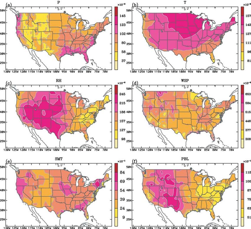
RSM. The RSM was initially developed by Juang and             (1991). As modified by Hong and Pan (1996), the RSM
Kanamitsu (1994; see also Juang et al. 1997) to provide       now allows convection to occur when the convective
a regional extension to the GSM, and thus in principle        available potential energy (CAPE) is large. There are
provides an almost seamless transition between the            some other important differences in the boundary
RSM and the GSM or the associated NCEP–NCAR                   layer. In the GSM boundary layer, vertical transfer is
reanalyses (Kalnay et al. 1996; Kanamitsu et al. 2002)        related to eddy diffusion coefficients dependent upon
and the higher-resolution region of interest. An intrin-      a Richardson number–dependent diffusion process
sic advantage, according to Hong and Leetma (1999),           (Kanamitsu 1989). In the RSM, a nonlocal diffusion
is that the RSM has relatively less restriction on nest-      concept is used for the mixed layer (diffusion coeffi-
ing size in comparison to other regional climate mod-         cients are still applied above the boundary layer).
els, and smaller nests can be easily embedded within          Briefly, in the mixed layer, the turbulent diffusion co-
the large-scale reanalysis or GSM forecasts with no-          efficients are calculated from a prescribed profile shape
ticeable errors or influences. For this experiment, the       as a function of boundary layer height and scale pa-
grid spacing was chosen to be 60 km at the central point.     rameters derived from similarity requirements (Troen
This horizontal resolution (and 18 vertical levels) is suf-   and Mahrt 1986). It should be noted that the RSM
ficient to resolve many features of interest, although        output planetary boundary layer height is actually the
eventually even higher-resolution simulations and fore-       height of the inversion layer, which can be a few tens
casts need to be attempted for the U.S. West, where           of meters higher than the commonly defined height
the topography exerts a strong control on near-sur-           corresponding to the level of maximum negative heat
face features.                                                flux, and the minimum height is the height of the low-
    Both the GSM and RSM use the same primitive               est model level (50 m), but nonetheless this PBL may
hydrostatic system of virtual temperature, humidity,          have some influence upon smoke and other pollutant
surface pressure, and mass continuity prognostic equa-        dispersal.
tions on terrain-following sigma (sigma is defined as             The RSM can be initialized directly from the GSM,
the ratio of the ambient pressure to surface pressure)        analysis or reanalysis, or it can use a previous integra-
coordinates. Therefore, in the absence of any regional        tion to initialize itself. Roads et al. (2003a) showed that
forcing (and intrinsic internal dynamics, any significant     it was best to initialize the RSM every day from the glo-
physical parameterization differences, and significant        bal analysis, since continuous runs adversely affected
spatial resolution) the total RSM solution should be          the regional solution. The first part of an RSM forecast
identical to the GSM solution. A minor structural dif-        or simulation involves the integration of the GSM for
ference is that the GSM utilizes vorticity and divergence     a nesting period based upon the large-scale output.
equations, whereas the RSM utilizes momentum equa-            Here, the RSM predicts regional deviations from the
tions in order to have simpler lateral boundary condi-        large-scale atmosphere base fields, which are linearly
tions. The GSM and RSM horizontal basis functions             interpolated in time between two output periods (6 h).
are also different. The GSM uses spherical harmonics          The nonlinear advection is first computed at the model
with a triangular truncation of 62 (T62) whereas the          grid points by transforming the global and regional
RSM uses cosine or sine waves to represent regional           spectral components to the regional grid. The global
perturbations about the imposed global-scale base             quantities are transformed to the global grid and then
fields on the regional grids. The double Fourier spec-        bilinearly interpolated to the regional grid; the regional
tral representations are carefully chosen so that the         quantities are exactly transformed. These calculations
normal wind perturbations are antisymmetric about             are almost exact (except for the interpolation error for
the lateral boundary. Other model scalar variables (i.e.,     the global quantities) and thus, like the global model,
virtual temperature, specific humidity, and surface log       the regional model is free of aliasing and phase error.
pressure) use symmetric perturbations.                        The linearly interpolated global-scale tendency is then
    Except for the scale-dependent horizontal diffusion,      removed, so that, in effect, only the portion affecting
the GSM and RSM physically are, in principle, identi-         the regional perturbation is retained. At the horizontal
cal. However, there are some notable parameteriza-            boundaries, the perturbation amplitude approaches
tion differences between the NCEP GSM and this RSM,           zero by a damping function increasing rapidly toward the
which has an upgraded physics package comparable              lateral boundary, which ensures that the boundary
to what was used for the NCEP Reanalysis II (see              tendencies are similar to the original GSM tendencies
Kanamitsu et al. 2002). Solar radiation is calculated         and features. A semi-implicit time integration scheme
from Chou and Suarez (1996) and the infrared radia-           is employed to suppress computational modes and also
tion is calculated according to Schwartzkopf and Fels         to allow the use of longer time integration steps.

AMERICAN METEOROLOGICAL SOCIETY                                                                 DECEMBER 2004           | 1889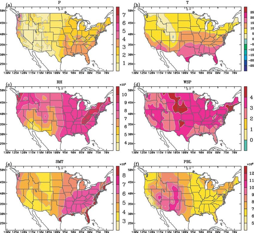
FIG. 1. Validating RSM annual means: (a) precipitation (P; mm day–1), (b) temperature (T; °C), (c) relative humidity (RH;
%), (d) wind speed (WSP; m s–1), (e) soil moisture (SMT; mm); and (f) planetary boundary layer height (PBL; m).

     Validations. We evaluated our 16-week GSM/RSM U.S.        latest high-resolution global model, or the reanalysis,
     forecasts, made starting every Saturday (0000 UTC)        which is based upon 4 times daily 6-h forecasts with
     since 27 September 1997. Again, an extensive valida-      the GSM, or the GSM 1-day forecasts (also output
     tion effort was previously undertaken for the GSM.        4 times daily) we previously used to validate the global
     Here we focus on the RSM forecasts, although some         model, but they do form a useful approximation that
     comparison to the coarser-scale GSM forecasts is also     can at least be used to estimate forecast skill. There
     provided. The main validation data for the weekly to      were very few (three) missing 0000 UTC initial states
     12-week forecasts was the weekly average of the 1-day     for the 5+ yr we have now run this experimental sys-
     RSM forecasts (output 4 times daily), initialized every   tem and for these periods we used a previous 2-day
     day from 0000 UTC analysis initial conditions and         forecast to generate the associated daily (actually 4 times
     bounded by the GSM 1-day forecasts (every 6 h). These     daily) GSM forcings.
     1-day RSM forecasts (also output 4 times daily) are not       Although the 1-day (output 4 times daily) RSM fore-
     exactly the same as the operational analysis, which is    cast validation set is certainly useful in the absence of
     based upon 4 times daily 6-h global forecasts from the    actual observations, at least there are better approxi-

1890 |      DECEMBER 2004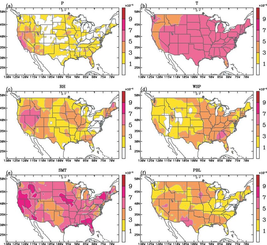
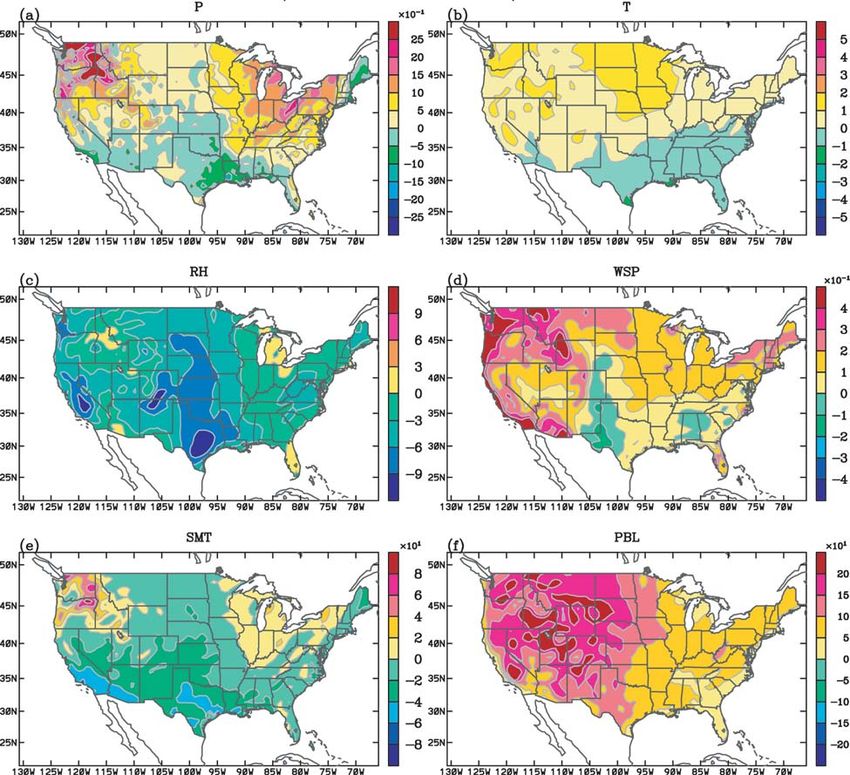
FIG. 2. RSM 12-week forecast systematic errors: (a) P (mm day–1), (b) T (°C), (c) RH (%), (d) WSP (m s–1), (e) SMT
(mm), and (f) PBL (m).

    mations to the U.S. precipitation from independent          certainly much less confident about other geophysical
    observations. For example, the National Climatic Data       variables (2-m RH, 10-m wind speed, total soil mois-
    Center (NCDC) and first-order station network along         ture in upper 2 m, and planetary boundary layer, or
    with the precipitation network of the River Forecast        more precisely height of inversion layer above lowest
    Centers were utilized by Higgins et al. (2000) to develop   model level). In that regard, the pending NCEP re-
    gridded (25 km) daily precipitation. Maximum and            gional reanalysis (Mesinger 2002) should eventually
    minimum temperature observations (Janowiak et al.           provide a better validation for these kinds of regional
    1999) were only available through September 2001,           model evaluations. In any event, the basic evaluation
    which would have limited our evaluation period to only      of these forecasts occurred for initial periods of 27 Sep-
    3 yr; however, as shown by Roads et al. (2003c), the        tember 1997 (since we also compared persistence fore-
    GSM and RSM surface temperature closely mimicked            casts, the first dynamical forecast actually began 4 Oc-
    these observations and we thus feel confident that our      tober 1997) with the ending validation day for the
    1-day RSM simulations provide an adequate substi-           16-week forecast ranging from 24 January 1998–12
    tute, for at least 2-m temperature. However, we are         January 2002.

    AMERICAN METEOROLOGICAL SOCIETY                                                              DECEMBER 2004           | 1891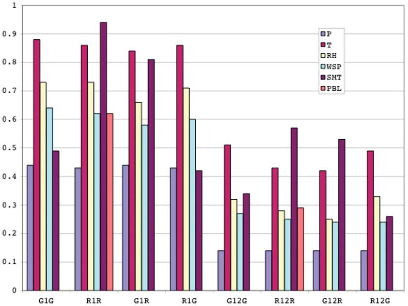
FIG. 3. Validating RSM 12-week standard deviations: (a) P (mm day–1), (b) T (°C), (c) RH (%), (d) WSP (m s–1), (e)
SMT (mm), and (f) PBL (m).

     Skill measures. The skill measures used here were pre-      the average of the temporal correlations is smaller
     viously used to describe the GSM forecast skill (e.g.,      than the average correlation. For this reason, a
     see RCF). Briefly they are                                  normalized covariance was used instead of the tem-
                                                                 poral spatial correlation when examining tempo-
     1) systematic error, which measures the average dif-        ral variations in the correlation; the average of the
        ference between forecasts and observations;              normalized covariances was then closer to the av-
     2) standard deviations, which compares the level of         erage correlation calculated over time and space.
        variation about the individual forecast and valida-
        tion climatologies;                                   GEOGRAPHICAL VARIATIONS. Figure 1 shows
     3) correlation, which compares the correlation be-       the annual means of the RSM validation data, which
        tween the forecast and validation anomalies: both     again consists of the average of 1-day RSM forecasts
        temporal and average correlations were computed       along with observed (Higgins et al. 2000) precipitation.
        and as pointed out by RCF, because there are times    Note that precipitation (P) is greatest over the north-
        when the entire domain is anomalously high or low,    west coastal regions and U.S. southeast, in contrast to

1892 |      DECEMBER 2004
FIG. 4. RSM 12-week forecast std dev in comparison to validating 12-week std dev. (a) P, (b) T, (c) RH, (d) WSP, (e)
SMT, and (f) PBL.
the drier central region of the Great Plains and U.S. general climatological features were quite similar in the
Southwest. Precipitation variations were quite similar GSM validation data (not shown).
to relative humidity (RH) and soil moisture (SMT) There were a number of noticeable systematic er-
variations, although RH and SMT were relatively rors (Fig. 2) in the RSM 12-week forecasts of the RSM
higher in the colder northern regions. In contrast to validation dataset. The precipitation was relatively large
precipitation, relative humidity, and soil moisture, 2-m in the north and relatively weak in the south. The 12-
temperature (T) decreased with latitude and elevation week temperature forecast was too high in the north
and had a more east–west orientation. Wind speed central and too low in the south. Wind speed (10 m)
(WSP) was strongest over the coastal regions in the lee had a strong systematic low bias in the Rocky Moun-
of the Rocky Mountains. The planetary boundary layer tain Front Range. For the most part, forecast soil mois-
height was a maximum over the dry mountainous re- ture was relatively dry just about everywhere but be-
gions of the United States [again the RSM had a diag- came especially dry in the southwest in the RSM and
nostic PBL, whereas the general circulation model especially dry throughout the intermountain region of
(GCM) did not]. Finally, it should be noted that these the West. Finally, the forecast PBL was relatively high,
AMERICAN METEOROLOGICAL SOCIETY DECEMBER 2004 | 1893FIG. 5. RSM 12-week forecast correlations: (a) P, (b) T, (c) RH, (d) WSP, (e) SMT, and (f) PBL.
especially over the western mountains, where it had a the country, where the land has a dominant influence
local maximum; this is somewhat consistent with the and the moderating ocean influences are smallest.
soil moisture forecasts, which were drier than the ini- Wind speed variability was strongest in the Northwest
tial state. The systematic errors in the GSM were some- and northern prairies.
what comparable to the RSM and will be discussed later Figure 4 shows that the forecast variations were
for the U.S. averages as a whole. relatively stronger than the validating analysis for al-
The validation standard deviations of 12-week most all variables except temperature. As noted by
means are shown in Fig. 3. Precipitation, soil moisture, Roads (2004), the precipitation variability was especially
and PBL variability were a maximum in the region strong over the U.S. West, in agreement with the overly
where they had maximum climatological values, namely strong GSM precipitation variability in this region (not
the northwest and southeast. Relative humidity, on the shown). This variability also showed up in the soil
other hand, was greatest in the southwest, presumably moisture variability, although interestingly, the vari-
because this is a dry region; in the moist regions, rela- ability was even stronger further to the east and south.
tive humidity is limited by the saturation value. Tem- The relative humidity variations were a bit strong in
perature variability was greatest in the central part of the Gulf Coast and Atlantic Seaboard and the wind
1894 | DECEMBER 2004speed variations were a bit strong in the region of the temporal variations of the U.S. 12-week RSM forecast
low-level jet, where the climatological values were rela- means (coterminous 48 states, cosine-weighted) in
tively weak by comparison. PBL variations were slightly comparison to the RSM validating data. For these and
strong everywhere, although the greatest excess vari- subsequent plots, individual 12-week means are plot-
ability occurred in the central part of the country. ted at the midpoint of the 12-week mean (e.g., the 12-
Figure 5 shows the correlations between the 12- week mean from 27 September 1997–19 December
week forecasts and the validating observations. Assum- 1997 is centered at 7 November 1997 on the plot ab-
ing 208 independent 12-week forecasts, correlations scissa). Despite obvious systematic errors, the fore-
above 0.1 might be considered to be significant at the casts and validations have similar seasonal and
99% level (e.g., Von Storch and Zwiers 1999). Of course, intraseasonal behavior. Temperature was a maximum
given the serial dependence of these forecasts, the sig- during the summer, in contrast to relative humidity,
nificance is likely to be lower. Anyway, temperature which was a maximum during the winter. Wind speed
forecasts were most skillful in the eastern part of the was a maximum during the winter–spring and a mini-
country where they were correlated with the RSM vali- mum during the summer–fall. Soil moisture was a
dations at greater than 60%; however, correlations were maximum during the spring and a minimum during
also greater than 0.4 for the western part of the coun- the fall. PBL was a maximum during the summer and
try. On the other hand, precipitation forecast correla- a minimum during the fall.
tions were greater than 0.1 only in the southern and Again, the mean or systematic errors were not in-
California regions of the country, where the ENSO cycle significant in either the GSM or RSM (Fig. 7). Although
dominates, and surprisingly has a north–south band the average RSM (solid lines) precipitation tends to
centered over the Great Plains. The correlations were follow the validating observations, there was a tendency
especially strong over California, indicating that this is for forecast precipitation to peak somewhat earlier, as
one region where we can make the best precipitation was noted previously by Roads et al. (2003a) and Roads
forecasts, at least during the wintertime. However, even (2004). The GSM (dashed lines) precipitation bias had
more skillful forecasts were made for the relative hu- a stronger seasonal cycle. Temperature errors were
midity, especially over the U.S. West, which has some relatively smaller although there was certainly a de-
implication for long-range forecasts of fire danger. Re- crease in error during the winter months, presumably
gions where the relative humidity forecasts were less in the southern tier of the United States. The GSM had
skillful, that is, over the U.S. East, were regions where a stronger positive bias during the wintertime. The rela-
the wind speed was forecast
best, which again could help to
provide some skill to forecasts
of fire danger, which depend
on both wind and relative hu-
midity (Roads et al. 1991). Soil
moisture was forecast well ev-
erywhere (presumably be-
cause this is a highly persistent
variable), with perhaps the dry
regions of New Mexico and
west Texas being the most dif-
ficult to accurately predict. Fi-
nally the planetary boundary
layer height was forecast best
across the southern tier of
states; it was more difficult to
forecast this variable to the
north, although there was
some indication of skill in the
northern prairies.
FIG. 6. RSM 12-week forecast (solid lines) and validation (dashed lines) U.S. aver-
TEMPORAL VARIA- ages: (a) P, (mm day–1), (b) T (°C), (c) RH (%), (d) WSP (m s–1), (e) SMT (mm),
TIONS. Figure 6 shows the and (f) PBL (m).
AMERICAN METEOROLOGICAL SOCIETY DECEMBER 2004 | 1895ter to summer transition. Soil
moisture variations were
quite similar in both the RSM
and GSM. Basically, the 12-
week forecasts were too dry,
especially during the late sum-
mer to fall. Twelve-week fore-
cast planetary boundary layer
heights were too high almost
all of the time, which was con-
sistent with the overall soil
moisture bias and at least the
positive summertime tem-
perature bias.
Figure 8 shows that the
magnitude of the temporal
variations of the U.S. stan-
dard deviations were compa-
rable to the magnitude of the
FIG. 7. RSM (solid lines) and GSM (dashed lines) 12-week forecast mean errors systematic errors, which is the
(U.S. average): (a) P (mm day–1), (b) T (°C), (c) RH (%), (d) WSP (m s–1), (e) main reason why one has to
SMT (mm), and (f) PBL (m). compute separate climatolo-
gies for different lagged fore-
casts. That is, comparisons of
the absolute differences
would be larger than the stan-
dard deviations; by taking
into account the climatologies
at different lags, we can focus
on the anomalous behavior,
which does have some fore-
cast skill. However, note that
variations in the 12-week
forecasts were much larger
than the variations in the vali-
dation dataset, especially in
the precipitation, relative hu-
midity, soil moisture, and
planetary boundary layer
height. Temperature and
wind speed had a better cor-
respondence between the
forecasts and validating data.
FIG. 8. RSM 12-week forecast (solid lines) and validation (dashed lines) U.S. std Figure 9 shows the tem-
dev: (a) P (mm day–1), (b) T (°C), (c) RH (%), (d) WSP (m s–1), (e) SMT (mm), poral variations of the corre-
and (f) PBL (m). lations for the RSM (solid
lines) and GSM (dashed lines)
12-week forecasts with the
tive humidity was relatively low in the RSM and RSM validations. Of interest here is how close the RSM
relatively high in the GSM although both showed some- and GSM forecast correlations were for all fields. For
what similar seasonal variations. The wind speed bi- some of the variables there was a clear seasonal varia-
ases were only slightly reduced in the RSM and both tion in skill. For example, precipitation and soil mois-
the GSM and RSM had too-strong winds during the win- ture forecast skill were strongest during the winter and
1896 | DECEMBER 2004smallest during the summer.
Of special interest is the slight
decrease in skill for many vari-
ables. RCF (see also Reichler
and Roads 2003) hypoth-
esized that part of the initial
forecast skill could probably
be attributed to the strong El
Niño–Southern Oscillation
(ENSO) cycle at the beginning
of the period.
FORECAST LAGS. Figure
10 shows the U.S. average sys-
tematic errors (in comparison
to the RSM validation) as a
function of forecast lead for
both the RSM (solid lines) and
GSM (dashed lines). RSM
(and GSM) precipitation were FIG. 9. RSM (solid lines) and GSM (dashed lines) 12-week forecast correlations
excessive initially, but became (U.S. average): (a) P (mm day–1), (b) T (°C), (c) RH (%), (d) WSP (m s–1), (e)
closer to the observations at SMT (mm), and (f) PBL (m).
long forecast lead times. In a
similar manner, the tem-
perature bias increased over
time. GSM RH had a positive
bias initially and then de-
creased toward a small bias at
long lead times, whereas the
RSM RH bias was small ini-
tially and then became a rela-
tively large negative basis at
long lead times. The soil
moisture also decreased with
increasing forecast time,
which had been noted previ-
ously by Roads and Chen
(2000). This decrease in soil
moisture is consistent with
the increasing bias in the PBL
height, although, as shown
previously, is not wholly geo-
graphically consistent. Finally
the wind speed had a slight
FIG. 10. U.S. RSM weekly (solid line) and GSM weekly (dashed) mean errors as a
negative bias in the RSM but a
function of forecast lead time (weeks): (a) P, (b) T, (c) RH, (d) WSP, (e) SMT,
small positive bias in the GSM. and (f) PBL.
Figure 11 shows the RSM
(solid lines) and GSM (dashed
lines) correlations with the RSM validation as a func- and RSM. The skill was especially high for the tempera-
tion of forecast lead. Also shown are RSM monthly (O) ture and soil moisture (although, as shown below, it is
and 12-week forecast correlations (*), and GSM actually quite difficult to diagnose this model-based
monthly (+) and 12-week (¥) forecast correlations. Note quantity). Precipitation appeared to be the most diffi-
that there is remarkable agreement between the GSM cult variable to forecast although wind speed and rela-
AMERICAN METEOROLOGICAL SOCIETY DECEMBER 2004 | 1897tive humidity were also rela-
tively difficult to forecast.
Except for soil moisture, all
variables show the positive
influence of time averaging,
indicating that forecasts of
time averages, even for lags
of 2 months, still show signifi-
cant skill. Note that 12-week
forecast skill at zero lag is also
almost as good as 4-week
forecasts at zero lag and only
slightly better than 12-week
averages at 1-month lag, in-
dicating the usefulness of dy-
namical models (in a time-
averaged sense) for seasonal
forecasts.
SUMMARY. Figure 12 sum-
FIG. 11. U.S. RSM weekly (solid line), monthly (o), 12-week (*), and GSM weekly marizes the GSM and RSM 1-
(dashed line), monthly (+), 12-week (x) forecast correlations: (a) P, (b) T, (c) and 12-week forecast corre-
RH, (d) WSP, (e) SMT, and (f) PBL.
lations using both the GSM
and RSM validation datasets
(observed precipitation was
used in place of daily forecast
precipitation in both data-
sets). Note that the weekly
forecast skill, as measured by
correlation, is quite high in
comparison to seasonal fore-
cast skill, which is especially
low for precipitation. Soil
moisture has fairly high skill
due to its remarkable persis-
tence, but there are obviously
problems in describing it; for
example, the global forecasts
were better able to forecast
the regional soil moisture
than the global soil moisture.
There does appear to be
somewhat of a scale problem
since the global model pre-
dictions of the regional vali-
dating set were generally
FIG. 12. GSM and RSM 1- and 12-week forecast correlations. G1G indicates 1- slightly lower than the re-
week forecasts made by the global model and validated by the global model vali- gional model predictions of
dations. R1R indicates 1-week forecasts made by the regional model and vali-
the global validating set (ex-
dated by the regional model validations. G1R indicates 1-week forecasts made
by the global model and validated by the regional model validations. R1G indi- cepting soil moisture). In any
cates 1-week forecasts made by the regional model and validated by the global event, despite the significant
model validations. Similar notation is applicable to the G12G, R12R, G12R, and skill of these seasonal fore-
R12G labels, except 12 denotes that these are 12-week forecasts. casts by the regional model of
1898 | DECEMBER 2004many geophysical variables, this skill
is certainly not significantly greater TABLE 1. RSM and GSM U.S. 1-week forecast means; forecast
than what might be achieved by a glo- systematic errors (SE); forecast std dev (SD); ratio of forecast
standard deviations to validating standard deviations (SD/SDv);
bal forecast model.
forecast correlations, using either the GSM or RSM validation
Although this paper emphasized datasets. G1G indicates 1-week forecasts made by the global
the evaluation of the RSM forecasts model and validated by the global model validations. R1R
(since a number of previous papers indicates 1-week forecasts made by the regional model and
had evaluated the GSM forecast skill), validated by the regional model validations. G1R indicates 1-
it has now become clear (see Tables 1 week forecasts made by the global model and validated by the
and 2) that the RSM has only compa- regional model validations. R1G indicates 1-week forecasts
rable but clearly not superior forecast made by the regional model and validated by the global model
validations.
capability over the corresponding
driving GSM. There were many simi-
larities. The 12-week GSM and RSM G1G Mean SE SD SD/SDv Correlation
precipitation was too high over the P, mm day-1 2.49 0.52 2.10 0.91 0.44
northern United States and deficient
T, K 283.31 -0.30 3.10 1.01 0.88
over the southern United States. By
contrast the soil moisture was too low RH, % 81.83 2.97 7.42 0.92 0.73
just about everywhere, except per- -1
WSP, m s 3.61 0.05 0.70 1.07 0.64
haps the northwest, where the 12-
week precipitation forecasts were ex- SMT, mm 480.18 -36.92 28.95 0.42 0.49
ceedingly wet. This dry soil moisture PBL, m
was consistent with an excessively
high U.S. West planetary boundary R1R Mean SE SD SD/SDv Correlation
layer (at least in the RSM). Forecast P, mm day -1
2.50 0.53 2.73 1.18 0.43
temperature was too low over the
T, K 283.08 -0.12 3.14 0.98 0.86
southern Gulf Coast states. Wind
speeds were too low in the southern RH, % 77.43 -0.56 7.74 1.01 0.73
entrance region of the low-level jet.
WSP, m s-1 3.58 0.18 0.66 1.12 0.62
The 12-week variations were compa-
rable to these 12-week forecast biases, SMT, mm 488.17 -0.73 30.52 1.11 0.94
indicating that they must be removed, PBL, m 833.87 65.67 176.41 1.07 0.62
either empirically or through the de-
velopment of better models. It should G1R Mean SE SD SD/SDv Correlation
also be mentioned that the RSM ap- P, mm day-1 2.49 0.52 2.10 0.91 0.44
pears to have somewhat greater vari-
ance, especially in the precipitation T, K 283.31 0.11 3.10 0.97 0.84
forecasts (see also Roads 2004) than RH, % 81.83 3.84 7.42 0.97 0.66
either the GSM or the validation -1
WSP, m s 3.61 0.21 0.70 1.18 0.58
dataset.
Thus, we have to conclude that the SMT, mm 480.18 -8.72 28.95 1.06 0.81
RSM is not yet capable of producing
PBL, m
quantitatively better weekly to sea-
sonal forecasts than the GSM. If we R1G Mean SE SD SD/SDv Correlation
can find ways to improve these RSM P, mm day -1
2.50 0.53 2.73 1.18 0.43
forecasts, perhaps by developing bet-
ter regional land surface initial condi- T, K 283.08 -0.53 3.14 1.02 0.86
tions or better regional parameteriza- RH, % 77.43 -1.43 7.74 0.96 0.71
tions, we may eventually be able to
show a clear advantage to using a re- WSP, m s-1 3.58 0.02 0.66 1.02 0.60
gional model for seasonal forecasts. SMT, mm 488.17 -28.93 30.52 0.44 0.42
This challenge is being met by the RSM
PBL, m
community of modelers, which has
AMERICAN METEOROLOGICAL SOCIETY DECEMBER 2004 | 1899shown steady growth for a number
TABLE 2. RSM and GSM U.S. 12-week forecast means; forecast of years (e.g., Roads 2000). In addi-
systematic errors (SE); forecast std dev (SD); ratio of forecast tion to the overall RSM model devel-
standard deviations to validating standard deviations (SD/SDv);
opment, which takes place as the
forecast correlations, using GSM or RSM validation. G12G
indicates 12-week forecasts made by the global model and
GSM is developed, increasing focus is
validated by the global model validations. R12R indicates 12- being paid to further improving RSM
week forecasts made by the regional model and validated by characteristics, which could then po-
the regional model validations. G12R indicates 12-week tentially influence further GSM de-
forecasts made by the global model and validated by the velopment. In that regard, it should
regional model validations. R12G indicates 12-week forecasts be mentioned that the evaluations
made by the regional model and validated by the global model described here were developed from
validations.
a somewhat older version of the RSM
(RSM96) and our goal is to begin
G12G Mean SE SD SD/SDv Correlation transitioning to the newer version of
P, mm day-1 2.42 0.46 0.81 1.09 0.14 the model (RSM), which is beginning
to show increased skill in some
T, K 283.82 0.12 1.62 0.98 0.51
regions.
RH, % 79.83 1.10 4.74 1.08 0.32 Finally, the RSM continues to pro-
-1 vide a potential outreach to the ap-
WSP, m s 3.57 0.02 0.29 1.32 0.27
plication community, which is inter-
SMT, mm 471.56 -44.03 35.17 0.84 0.34 ested in not only the long forecast
PBL, m horizons and ensembles currently
obtainable from global models, but
R12R Mean SE SD SD/SDv Correlation also the higher geographic resolution
P, mm day -1
2.39 0.43 0.99 1.33 0.14 obtainable from regional models.
Again, besides possible influences
T, K 283.78 0.48 1.65 0.98 0.43
upon regional skill, another value of
RH, % 74.08 -3.84 5.01 1.28 0.28 regional model simulations and fore-
casts is the increased scrutiny brought
WSP, m s-1 3.54 0.15 0.26 1.32 0.25
to bear for a specific region. It is now
SMT, mm 477.58 -10.90 39.06 1.75 0.57 possible to use a small amount of glo-
PBL, m 886.91 119.56 89.70 1.26 0.29
bal or regional analysis data to initial-
ize and drive a regional model on
G12R Mean SE SD SD/SDv Correlation short to long time scales. We can then
P, mm day-1 2.42 0.46 0.81 1.09 0.14 use these regional models to provide
comprehensive regional output and
T, K 283.82 0.53 1.62 0.97 0.42 to examine various physical param-
RH, % 79.83 1.90 4.74 1.21 0.25 eterizations and test various scientific
-1
hypotheses under highly controlled
WSP, m s 3.57 0.18 0.29 1.46 0.24
boundary conditions. Regional mod-
SMT, mm 471.56 -16.92 35.17 1.57 0.53 els thus continue to provide a valu-
able analysis tool, even if they are
PBL, m
not yet able to provide a superior
R12G Mean SE SD SD/SDv Correlation long-range forecast tool. Our chal-
P, mm day -1
2.39 0.43 0.99 1.33 0.14 lenge is still to show that the RSM and
other regional models can signifi-
T, K 283.78 0.08 1.65 1.00 0.49 cantly contribute to global seasonal
RH, % 74.08 -4.64 5.01 1.15 0.33 forecast ensembles and global
change experiments.
WSP, m s-1 74.08 -4.64 5.01 1.15 0.33
SMT, mm 3.54 -0.02 0.26 1.19 0.24 ACKNOWLEDGMENTS. This re-
search was funded by a cooperative
PBL, m 477.58 -38.01 39.06 0.94 0.26
agreement from NOAA-NA17RJ1231,
1900 | DECEMBER 2004and NASA NAG5-11738, and a cooperative agreement with ——, and A. Leetmaa, 1999: An evaluation of the NCEP
the USFS (USDA 02-JV-11272169). The views expressed RSM for regional climate modeling. J. Climate, 12,
herein are those of the authors and do not necessarily re- 592–609.
flect the views of NOAA, NASA, or USFS. I thank J. Ritchie Janowiak, J., G. Bell, and M. Chelliah, 1999: A gridded
for his help with the computations, and M. Kanamitsu, database of daily temperature maxima and minima
S. Chen, F. Carr, and the anonymous reviewers for their for the conterminous US: 1948–1993. NCEP Climate
useful comments. Prediction Center Atlas Rep. 6, 35 pp.
Juang, H., and M. Kanamitsu, 1994: The NMC nested
regional spectral model. Mon. Wea. Rev., 122, 3–
REFERENCES 26.
Anderson, B. T., and J. O. Roads, 2002: Regional simu- ——, S. Hong, and M. Kanamitsu, 1997: The NMC
lation of summertime precipitation over the south- nested regional spectral model. An update. Bull.
western United States. J. Climate, 15, 3321–3342. Amer. Meteor. Soc., 78, 2125–2143.
——, ——, and S.-C. Chen, 2000a: Large-scale forcing Kalnay, E., and Coauthors, 1996: The NCEP/NCAR 40-
of summertime monsoon surges over the gulf of Year Reanalysis Project. Bull. Amer. Meteor. Soc., 77,
california and southwest United States. J. Geophys. 437–471.
Res., 105, 455–467. Kanamitsu, M., 1989: Description of the NMC global
——, ——, ——, and H.-M. H. Juang, 2000b: Regional data assimilation and forecast system. Wea. Fore-
simulation of the low-level monsoon winds over the casting, 4, 335–342.
gulf of california and southwest United States. J. ——, W. Ebisuzaki, J. Woolen, J. Potter, and M. Fiorino,
Geophys. Res., 105, 17 955–17 969. 2002: NCEP/DOE AMIP-II Reanalysis (R-2). Bull.
——, ——, ——, and ——, 2001: Model dynamics of Amer. Meteor. Soc., 83, 1631–1643.
summertime low-level jets over northwest Mexico. Leung, L. R., Y. Qian, J. Han, and J. O. Roads, 2003:
J. Geophys. Res., 106, 3401–3413. Intercomparison of global reanalyses and regional
Chen, S.-C., 2002: Model mismatch between global and simulations of cold season water budgets in the
regional simulation. Geophys. Res. Lett., 29, 1060, western U.S. J. Hydrometeorology, 4, 1067–1087.
doi:10.1029/2001GL013570. Marshall, S., J. O. Roads, and R. J. Oglesby, 1997: Ef-
——, J. O. Roads, H.-M. H. Juang, and M. Kanamitsu, fects of resolution and physics on precipitation in
1999: Global to regional simulation of California’s the NCAR Community Climate Model. J. Geophys.
wintertime precipitation. J. Geophys. Res., 104, 31 Res., 102, 19 529–19 541.
517–31 532. Mesinger, F., and Coauthors, 2002: NCEP regional re-
——, ——, and M. Wu, 2001: Seasonal forecasts for analysis. Preprints, Symp. on Observations, Data As-
Asia: Global model experiments. J. Terr.–Atmos.– similation, and Probabilistic Prediction, Orlando,
Oceanic Sci., 12, 377–400. FL, Amer. Meteor. Soc., J59–J63.
——, M.-C. Wu, S. Marshall, H.-M. H. Juang, and J. O. Reichler, T. J., and J. O. Roads, 2003: The role of
Roads, 2003: 2xCO 2 Eastern Asia Regional Re- boundary and initial conditions for dynamical sea-
sponses in the RSM/CCM3 Modeling System. Glo- sonal predictability. Nonlin. Processes Geophys., 10,
bal Planet. Change, 37, 277–285. 1–22.
Chou, M.-D., and M. J. Suarez, 1996: A solar radia- Roads, J. O., 2000: The Second International Regional
tion parameterization (CLIRAD-SW) for atmo- Spectral Model Workshop. Bull. Amer. Meteor. Soc.,
spheric studies. NASA Tech. Memo. 104606, v. 15, 81, 2979–2982.
48 pp. ——, 2004: Experimental weekly to seasonal, global to
Han, J., and J. Roads, 2004: US climate sensitivity sim- regional US precipitation forecasts. J. Hydrol., 288,
ulated with the NCEP regional spectral model. 153–169, doi:10.1016/j.jhydrol.2003.11.033
Climate Change, 62, 115–154, doi:10.1023/ ——, and S.-C. Chen, 2000: Surface water and energy
B:CLIM.0000013675.66917.15 budgets in the NCEP regional spectral model. J.
Higgins, R., W. Shi, E. Yarosh, and R. Joyce, 2000: A Geophys. Res., 105, 29 539–29 550.
gridded precipitation database for the United States ——, and S. Brenner, 2002: Global model seasonal fore-
(1963–1993). NCEP Climate Prediction Center At- casts for the Mediterranean region. Israel J. Earth
las Rep. 7, 47 pp. Sci., 51, 1–16.
Hong, S., and H. Pan, 1996: Nonlocal boundary layer ver- ——, and S.-C. Chen, 2003: Evaluation of seasonal fore-
tical diffusion in a medium-range forecast model. cast skill over China. Global Planet. Change, 37, 327–
Mon. Wea. Rev., 124, 2322–2339. 335.
AMERICAN METEOROLOGICAL SOCIETY DECEMBER 2004 | 1901——, K. Ueyoshi, S.-C. Chen, J. Alpert, and F. Fujioka, ——, and Coauthors, 2003c: GCIP water and energy
1991: Medium-range fire weather forecasts. Int. J. budget synthesis (WEBS). J. Geophys. Res., 108, 8609,
Wildland Fire, 1, 159–176. doi:10.1029/2002JD002583.
——, S. Chen, M. Kanamitsu, and H. Juang, 1999: Sur- ——, S. Chen, F. Fujioka, and R. Burgan, 2004: Seasonal
face water characteristics in NCEP global spectral fire danger forecasts for the USA. Int. J. Wildland
model reanalysis. J. Geophys. Res., 104, 19 307–19 327. Fire, Special Issue: Fire and Forest Meteorology, in
——, ——, and F. Fujioka, 2001a: ECPC’s weekly to sea- press.
sonal global forecasts. Bull. Amer. Meteor. Soc., 82, Schwarzkopf, M. D., and S. B. Fels, 1991: The simpli-
639–658. fied exchange method revisited: An accurate, rapid
——, B. Rockel, and E. Raschke, 2001b: Evaluation of method for computation of infrared cooling rates
ECPC’s seasonal forecasts over the BALTEX region and fluxes. J. Geophys. Res., 96, 9075–9096.
and Europe. Meteor. Z., 10, 283–294. Takle, E. S., and Coauthors, 1999: Project to Intercom-
——, S.-C. Chen, and M. Kanamitsu, 2003a: U.S. re- pare Regional Climate Simulations (PIRCS). J.
gional climate simulations and seasonal forecasts. Geophys. Res., 104, 19 443–19 461.
J. Geophys. Res., 108, 8606, doi:10.1029/2002JD002232. Troen, I., and L. Mahrt, 1986: A simple model of the
——, ——, L. Druyan, M. Fulakeza, S. Cocke, T. LaRow, atmospheric boundary layer: Sensitivity to surface
J.-H. Qian, and S. Zebiak, 2003b: International Re- evaporation. Bound.-Layer Meteor., 37, 129–148.
search Institute/Applied Research Centers (IRI/ Von Storch, H., and F. W. Zwiers, 1999: Statistical
ARCs) regional model intercomparison over South Analysis in Climate Research. Cambridge Univer-
America. J. Geophys. Res., 108, 4425, doi:10.1029/ sity Press, 216 pp.
2002JD003201.
1902 | DECEMBER 2004You can also read