The most advantageous partners for Australia to bilaterally link its emissions trading scheme - NZAE
←
→
Page content transcription
If your browser does not render page correctly, please read the page content below
The most advantageous partners for Australia to
         bilaterally link its emissions trading scheme

                                      Duy Nong
                     UNE Business School, University of New England
                            Armidale, NSW, Australia 2350
                             Email: nnong@myune.edu.au

                                 Mahinda Siriwardana
                     UNE Business School, University of New England
                            Armidale, NSW, Australia 2350
                              Email: asiriwar@une.edu.au

Abstract

The theory of marginal abatement cost (MAC) indicates that if a country has a high MAC, it
should link its domestic emissions trading scheme (ETS) with a foreign country which has
either low MAC or low emissions reduction target. This is required to maximise its economic
benefits from the linkage compared to its domestic ETS. On the other hand, if a country has a
low MAC, it would seek a partner which has either a high MAC or a high emissions
reduction target. Using a computable general equilibrium (CGE) model, namely the extended
GTAP-E model, the authors found that Australia would yield the greatest economic benefits
by linking its ETS with India. China is the second best alternative for Australia to link its
ETS while the European Union is the most expensive option for Australia. However, any
bilateral linkage is always better for Australia than operating its own domestic ETS.

Keywords: Australia, emissions trading scheme, linkage, marginal abatement cost, CGE
model.

JEL classification codes: F18, Q56, Q58.

1 Introduction

Since the last decade, many policy makers have been considering an emissions trading
scheme (ETS) as a promising policy to tackle climate change issues. There are many schemes
currently operating around the world. They include regional ETS in the European Union
(EU), national ETSs in Switzerland, Norway, Kazakhstan, New Zealand and South Korea,
and many other regional schemes in United States, Canada and Japan (Parliament of
                                              1!
!
Australia, 2013b). Many researchers have concluded that such schemes not only have
moderate effects on economies but also bring great benefits to economic systems (Adams,
2007; Adams et al., 2014; Babiker et al., 2004; Hawkins & Jegou, 2014; Tuerk, 2009). The
benefits would be larger if the borders of the schemes are broader. In this regard, several
governments have shown their ambition to establish a global emissions trading market
because of many advantages from such linkages (European Commission, 2016; Hawkins &
Jegou, 2014; Ranson & Stavins, 2015; Siriwardana, 2015). In Australia, the Labor
Governments (Rudd 2007-10; Gillard 2010-13; Rudd 2013) had negotiated with the
European Union to link the Australian ETS with the EU-ETS after the success in
implementing the Carbon Price Mechanism in the domestic market (Deparment of Climate
Change and Energy Efficiency, 2012). Under these negotiations, the first stage (2015-18)
would be a one-way link where the liable entities in Australia would import allowances from
the EU-ETS. From 2018, these two schemes were intended to develop two-way links. In the
proposal, the Australian Labor Government also desired to negotiate with other countries in
order to link with its ETS (Parliament of Australia, 2013a).

The most significant benefit of the linkage is the opportunity to reduce the total costs of
abatements in comparison to operating their own domestic ETSs alone. In a linkage,
participants will jointly seek to equalise their marginal abatement costs (MACs) hence the
price of permits will converge to an intermediate level. Such an outcome leads to an increase
in market liquidity and a decrease in concern for an emissions leakage and unfair
competiveness between participants when every firm in the linkage faces the same price for
permits (M. Babiker et al., 2004; Flachsland, Marschinski, & Edenhofer, 2009; Hawkins &
Jegou, 2014; Jaffe & Stavins, 2008; Siriwardana, 2015; Tuerk, 2009). Using a graphical
illustration to show the cost-effectiveness achieved by an international ETS, Babiker et al.
(2004) pointed out that two countries in the linkage would equalise their MACs and both
economies would achieve net economic gains through the linkage.

In order to carry out such a comparison of benefits, it is assumed that the proposed economies
have their own domestic cap-and-trade ETSs and they are compatible in order to unify their
domestic ETSs into an international ETS. In each scheme, permits are entirely auctioned. In
this paper, the authors will compare the potential economic benefits gained by Australia from
a bilateral ETS linkage with the European Union, United States, South Korea, Japan, China
and India. We assume the implementations of the schemes in these selected economies could

                                               2!
!
be a promising policy for governments to pursue following the agreements at the 2015 Paris
Climate Conference. In addition, if an ETS was implemented in Australia, the first process
would likely be the negotiations for bilateral trades with other schemes. In order to complete
such comparisons, we use the computable general equilibrium (CGE) modelling approach,
namely the extended GTAP-E model. This model particularly suits this task, as it includes
complete interactions between consumers and producers throughout the world. Bilateral
trades between countries are also presented in the model. In addition, it consists of
greenhouse gas emissions in the database, which is released from the production processes
and consumption of fuels. Furthermore, the model provides a mechanism to implement ETSs
in different economies and a possibility of linking such ETSs.
In this study, the emissions targets for these economies are considered according to their
plans for 2030 which they were committed at the 2015 Paris Climate Conference. The
analysis focuses assuming that these ETSs are implemented in markets where there are no
pre-existing distortions1. This is because the problem of “immiserizing growth” occurs when
there are pre-existing distortions in partner economies (Bhagwati, 1958; Lipsey & Lancaster,
1956), hence not all countries benefit from a linkage of ETSs (Babiker et al., 2004).
The paper is organised as follows. Section 2 describes the theory of marginal abatement cost
in the context of international ETS and a review of previous literature is in Section 3. Section
4 outlines the model, database and emissions targets used in this study. Section 5 presents the
simulation results and discussions. Section 6 concludes the paper.
2 Marginal abatement cost
Marginal abatement costs normally differ between countries. In some economies, MAC
would increase considerably if they undertake a small amount of additional emissions
reduction. However, some other economies would experience only low levels of MAC for
every additional unit of abatement. Some of the main reasons for differential MACs between
countries are energy efficiency, possibilities of fuel substitutions and sources of emissions. If
a country can improve technology in order to use energy more efficiently, their MAC will
become lower. In addition, the higher the possibility to substitute clean energy sources (e.g.
natural gas) for emissions intensive energy inputs (e.g. coal), the greater the potential for a
!!!!!!!!!!!!!!!!!!!!!!!!!!!!!!!!!!!!!!!!!!!!!!!!!!!!!!!!
1
Distortions in a market occur when there are existing taxes, such as taxes on fossil fuels. In addition, such
taxes are different from country to country (Babiker et al., 2004).
3!
!country to achieve a lower MAC. If a country burns a large amount of fossil fuels in their
production processes, a small improvement in technology to switch to clean energy inputs or
use of energy more efficiently would enable that country to reduce its MAC considerably.
The source of emissions is also an important component to determine the MAC. If a country
has a high level of emissions from production processes, it is unlikely that it will have a low
MAC as it has to reduce the level of production in order to lower its emissions levels. Labour
and capital costs are also major determinants of the MAC level of a country. If such costs are
low, it is not costly for the country to reduce its production level, thus diminishing the
emissions levels in order to meet a target. Production sectors can also substitute capital for
energy when the price of energy increases considerably. As a result, such a country will pay
less for every tonne of abatements.
When ETSs are linked together in an international ETS, participants could reduce the total
cost of abatements by equalising their MACs. In such a linkage, all countries or regions will
achieve economic benefit buts linkage with different partners will yield different benefits to
the country. In this regard, Figure 1 graphically shows the cost-effectiveness of an
international ETS with two countries.
Figure 1: Cost-effectiveness of an international ETS
(a) (b)
MAC1
Permits Permits
price price
MAC1
A’ MAC3
B
P1 A P1
MACT
P*
B MAC2 P2
MACT
P*
P2
Q11 Q1 Q2 Q22 QT Q11 Q1 Q3 Q33 QT Emissions
Emissions
reduction reduction
Source: Adapted from Babiker et al. (2004).
Figure 1 (a) indicates that country 1 and country 2 initially perform their domestic ETSs.
Country 1 commits to reduce its emissions levels by Q1 units under its regulation while
4!
!country 2 reduces its emissions levels by Q2 units. In addition, country 1 has a relatively high
MAC, which is indicated by MAC1 curve while country 2 has a lower MAC curve, namely
MAC2. Under two independent schemes, country 1 has a higher price of permits than it is for
country 2 (P1 > P2) because country 1 has higher MAC than in country 2. When these two
countries link their domestic ETSs, they jointly obtain a lower MAC (indicated by MACT)
relative to their individual MAC curves. Total emissions reduction units for such a linkage
are QT (= Q1 + Q2). As shown in Figure 1 (a), the linkage allows the two countries to obtain
an intermediate price for permits (P*). Of these, the high emissions abatement cost country
(country 1) will only reduce its emissions by Q11 units and buy additional permits (= Q1 –
Q11) from country 2. In such a case, country 2 will reduce its emissions by Q22 units and sell
its surplus permits (= Q22 – Q2) to country 1 where Q22 – Q2 is equal to Q1 – Q11. As a result,
such a linkage enables both country 1 and country 2 to achieve the net economic gains
(marked by area A and area B, respectively) compared with their own domestic schemes.
The net gains, area A and area B, however, are subject to change due to a change in partners
or emissions targets (or abatement units). For example, if country 2 in Figure 1 (a) reduces its
emissions targets or expects to achieve a lower level of emissions reduction units, the total
abatement units (QT) will decline, hence decreasing the price of permits and increasing the
net gain (area A) for country 1. Similarly, if country 2 increases its emissions reduction units,
it will reduce net gain for country 1. By contrast, the higher the level of emissions reduction
in country 1 the greater the net gains (area B) country 2 will achieve. Figure 1 (b) shows that
country 1 links its ETS with country 3, which has the same emissions reduction target as
country 2 (Q3 = Q2) but higher MAC relative to country 2 (MAC3 > MAC2). With the same
analysis as in Figure 1 (a), country 1 only achieves the net gain A’, where area A’ is smaller
than area A in Figure 1 (a). These illustrations suggest that if country 1 is a high MAC
country, it should link its domestic ETS with a scheme, which has either a low MAC or a low
emissions reduction target, in order to maximise its economic benefits from the linkage
compared with its domestic ETS. On the other hand, a low MAC economy like country 2
would seek a partner, which has either a high MAC or a high emissions reduction target.
3 Survey of literature
Studying the effects of the environmental taxes on different economies has been well
developed, especially since the use of CGE models for environmental policy analysis.
Economists and environmentalists therefore have reliable tools to quantify the comprehensive
5!
!effects of such policies on various aspects of an economy. Recently, there has emerged a
wide range of empirical literature that develops applications of CGE modelling in order to
estimate the effects of ETSs. Many studies have focused on the European Union ETS (EU-
ETS) subject to the Kyoto Protocol commitment. For example, Böhringer (2002) used a
world CGE model to examine the effects of the restricted levels for trading emissions on the
magnitude and distribution of abatement costs across EU countries. The model encompasses
7 sectors and 23 regions, including 15 EU member states. The database for the model was
constructed from four sources with a base year of 1995. Of these, GTAP4 contains global
Input-Output tables; EUROSTAT includes Input-Output tables for all EU member countries;
IEA provides energy balances and energy prices/taxes; and CHELEM supplies harmonized
accounts on bilateral trade between countries. The author found that allowing for the
possibility of trading between power sectors across country borders would provide the
highest efficiency gains, instead of restricting them to domestic markets subject to the
electricity sectors receiving permits at an auction price, rather than free.
Babiker et al. (2003) used the Emissions Prediction and Policy Analysis European Union
(EPPA-EU) model in order to examine (1) how the allocation of emissions permits between
sectors affect the welfare costs in the European Union and (2) the effects of the climate
change strategy on domestic production. Such a model is a global dynamic general
equilibrium model, which includes 11 sectors and 22 regions. The simulation results
indicated that permit allocations would lower economic costs if such allocations differ from
the trading solution in the simulations while the European economy would bear more costs in
the case of exempting energy-intensive industries. The findings also suggest that divergence
from the domestic economy-wide cap-and-trade system increases economic costs but the EU
economy is better off rather than having an economy-wide cap-and-trade system due to
existing energy taxes in the various economies.
Kemfert et al. (2006) used the GTAP-E model in order to analyse the abatement costs and
welfare impacts of the EU-ETS. The GTAP-E model is a static multi-country and multi-
sector CGE model. There are three scenarios in this study. In Scenario 1, the emissions quota
for each selected sector of each region was fixed, the carbon prices were then determined
endogenously. There was no trading of emissions in this scenario. Scenario 2 allowed
emissions trading between sectors within each country’s border. In Scenario 3, all selected
sectors could trade their permits within the EU region. The permit allocations were based on
6!
!the national allocation plans2 as submitted to and approved by the EU. The simulation results
show that the real GDP increased in all regions while welfare gains mostly occurred in
regions where high efficiency gains from emissions trading were experienced. When
emissions permits were allowed to trade across the borders, the abatement costs for all EU
States members were relatively low (at US$2 per tonne of CO2). In such a trading scenario,
Germany, UK and the Czech Republic were the main sellers of emissions permits, whereas
Belgium, Denmark, Finland and Sweden became the main buyers.
Edwards and Hutton (2001) applied a CGE model in order to compare the economic effects
of different methods of permits allocation within the UK, subject to a target (i.e. reducing the
UK’s emissions level by 17.5% relative to business-as-usual). This CGE model consists of 12
perfectly competitive sectors, nine being fuels and three non-energy. The authors assumed
that the permits were traded internally in the UK market. The main findings included (1) if
revenue from permit auction is recycled to industry through output subsidies or employment
tax cuts, it is likely to cause a ‘double dividend’. (2) When permits are allocated freely, the
cost is increased if foreign-owned companies consider such permits as a windfall to repatriate
to shareholders. However, in the case of free allocation using benchmarks, it is not
necessarily costly. (3) The 2010 UK’s emissions target needed much tighter controls beyond
2010, especially as a rapid growth in carbon use outside the Organisation for Economic Co-
operation and Development area was expected. In that case, the authors suggested that taxes
and permit prices could be much higher than the price levels found in the study.
Kim et al. (2004) used a CGE model to evaluate the effects of the dual system of carbon tax
and ETS on South Korea’s economy. Such a model is a multi-sector recursive dynamic CGE
model, which includes 21 goods and services. The ETS was applied for large emitters while a
carbon tax was applied for small emitters. Two cases of emissions reduction were considered
in this study. They are a 20% reduction target scenario and 1995 emissions level stabilization
scenario. The results show that the targets could be achieved in both scenarios via the dual
system. In addition, MACs of large emitters would increase faster than those for small
emitters in South Korea. The authors concluded that the carbon tax along with an ETS would
be the most efficient option for South Korea to reduce emissions if the carbon tax and the
price of permits were applied to emitters according to their levels of marginal cost.
!!!!!!!!!!!!!!!!!!!!!!!!!!!!!!!!!!!!!!!!!!!!!!!!!!!!!!!!
2
A national allocation plan determines how many allowances to be allocated in total and to each EU ETS
installation on their territory.
7!
!There were also many studies, which applied the CGE models to assess the effects of an ETS
on the Australian economy. The ETS was either applied in the domestic market only or as a
part of the global or international emissions trading market. For example, Adams (2007) used
the Monash Multi-Regional Forecasting (MMRF) model with key inputs related to the
electricity sector supplied by McLennan, Magasanik Associates (MMA) in order to evaluate
the likely costs of an ETS on the Australian economy. The MMRF model is a dynamic model,
containing 52 industries, 56 commodities, 8 states/territories and 56 sub-state regions of
Australia. Of these, the outputs of the MMA model were the inputs in the MMRF model.
Adams suggested that the ETS should be introduced in Australia, as the economy would
grow strongly in the case of ETS. Adams also indicated that the compensation for energy cost
increases could allow maintenance of global trade competitiveness for Australian producers.
In addition, the impacts on economic welfare could be moderated via targeted recycling of
revenue from auctioned permits.
Gerardi and Demaria (2008) quantified the impacts of the Carbon Pollution Reduction
Scheme (CPRS) on the Australia’s electricity generation sectors by using an integrated CGE
modelling approach. Such an approach includes a suite of models, such as the GTEM model
(outlined the international impacts), the MMRF model (detailed the domestic impacts) and
the MMA’s electricity market models (presented the sectoral impacts). In this approach,
outputs of the other modelling simulations were key inputs into the electricity market
simulations. The simulation results indicate that the emissions levels of the Australian
electricity sectors in all policy scenarios were far lower than the emissions level projected in
the baseline. They also found that there was a strong transition to renewable energy industries
in Australia. Such renewable energy production was predicted to contribute half of the
generation mix by 2050.
Hoque et al. (2010) used the MMRF-Green model in order to assess the impacts of the
CPRS-53 on the Australian economy, particularly the tourism sectors. As the tourism sector is
not disaggregated in the database, the authors obtained the effects on the Australian tourism
industry by linking the MMRF-Green model and Tourism Satellite Account (TSA) 4
methodology. That is, the authors had to map the industry in the TSA and MMRF-Green
!!!!!!!!!!!!!!!!!!!!!!!!!!!!!!!!!!!!!!!!!!!!!!!!!!!!!!!!
3
The CPRS is an emissions trading scheme for GHG emissions, which the Australian government proposed to
commence in 2011. The CPRS-5 scenario indicates that a cap on the Australian emissions is set at 475 Mt in
2020, that is 5% below the 2000 level (of 500 Mt) by 2020.
4
A TSA provides macroeconomic aggregates that describe the size and the economic contribution of tourism
output, tourism direct gross value added and tourism direct gross domestic product, consistent with similar
aggregates for the total economy, and for other productive economic activities.
8!
!model industry. In the modelling, an initial price of emissions of A$25 per tonne was
imposed in 2011 and the Australian industries could buy emissions permits from the
international markets in order to meet their national obligations. The projections were
obtained until 2020. As a result, Australia only experiences a mild contraction in the
economy at the macro level compared with the baseline scenario. Most tourism industries
would only experience small contractions in their real outputs and some industries would
undergo expansion. Among them, the most adversely affected industries were cafes,
restaurants and food outlets, air transport, and water transport with reductions in outputs by
1.32%, 1.32% and 0.82%, respectively. The most favourably affected sector was rail
transport with an expansion in activity by 1.28%, as it is a low emissions intensive industry.
In 2011, the Australian Treasury (2011) released a comprehensive analysis of the carbon
pricing in Australia by using the CGE modelling approach. The analysis was based on the
simulation results from a combination of many models, such as two top-down dynamic CGE
models (the GTEM and MMRF models); bottom-up sector-specific models for electricity
generation and road transport sectors; a partial-equilibrium model of the Australian energy
sector (the Energy Sector model); the model for estimating the impact of the Carbon Farming
Initiative on the Australian forestry sector; the Treasury’s Price Revenue Incidence
Simulation model (to quantify the effects of a carbon price on a range of prices); and the
Treasury’s Price Revenue Incidence Simulation model and Distribution model (to analyse the
distributional implication for households). In Scenario 1, carbon price was assumed to start
from A$20 per tonne in 2012-13, rising 5% per year, projected to be around A$29 in 2015-
16. In Scenario 2, the starting carbon price in 2012-13 was assumed to be at A$30 per tonne,
rising to A$61 in 2015-16. In both modelling scenario results, the real income of Australia
still grew but at a slightly diminishing rate, as the domestic economy transforms to be more
carbon efficient and as sourcing international abatement causes income outflow. Pricing
carbon affected the demand for labour as a result of slower output and capital growth,
however, the level of employment was unaffected. Labour moved across industries during the
transition to a lower carbon economy, although the rate of movement was relative low
compared to normal rates of job turnover from year to year. In this study, pricing carbon
would considerably change the composition of electricity generation in Australia. Electricity
generation from renewable sources was estimated to be higher in both scenarios. Renewable
generation would rise by 20% and 21-26% of total electricity generation output by 2020
under Scenario 1 and Scenario 2, respectively. Wind generation would develop quickly
9!
!initially, then it would be overtaken by geothermal energy generation. The results also
indicated that gas would play an important role in generating electricity in Australia in both
scenarios.
Adams et al. (2014) investigated the effects of an ETS on the Australian electricity sector.
The ETS in Australia was a part of the global ETS. Hence, the dynamic multi-country CGE
model, namely the GTEM model was used to generate the prices and allocations of permits
for Australia. The outputs were then the inputs in the MMRF model. In addition, the
electricity sector in MMRF was replaced by the WHIRLYGIG’s specification. The
WHIRLYGIG model includes detailed information of the Australian electricity sectors,
including wholesale and retail electricity prices, capacity by generation type, fuel use,
emissions, etc. The main findings were that the global price of permits increased from A$25
per tonne in 2015 to A$50 in 2030, Australia would need to buy half of its abatement
required from overseas markets and Australia would only experience a reduction in GDP by
1.1% in 2030 relative to the baseline.
Siriwardana (2015) used the GTAP-E model in order to assess the effects of ETSs linkage
between Australia, Japan and South Korea on their economies and emissions levels. The
linkage was carried out as a complement to the free trade agreements (FTAs) between
Australia and the other two countries. The GTAP-E model is a static multi-region and multi-
sector CGE model. Two scenarios were examined in his study. In Scenario 1, the simulation
was performed by cutting all bilateral tariffs between Australia and the other two countries.
Scenario 2 was carried out with an additional ETSs linkage between these three economies.
The emissions quota or target for each of the three countries followed the 2020 targets,
ratified at the Cancun conference in 2010. Such 2020 targets were then converted into targets
in the base year 2007. The author found that removing bilateral protection of trade brings
significant benefits to all three countries. Real GDP and welfare in these three countries were
likely to increase. However, when the FTAs were under operation with the complement of
the ETSs, real GDP of these three countries were reduced considerably (e.g. -3.69% for
Australia, -2.43% for Japan and -3.52% for South Korea). The price of permits was also very
high. Based on such findings, the author indicated that an ETS linkage between Australia,
Japan and South Korea would be a very expensive option, as all three countries would lose
their competitive advantage.
10!
!4 Model and database
4.1 Model structure and database
This study uses an extended GTAP-E model in order to quantify the net economic gains for
Australia from different bilateral ETS linkages. In GTAP-E, consumers are modelled to
maximise utility, while firms or producers will try to minimise costs. The model also contains
market-clearing conditions, where supplies of goods and services are equal to demands. In
addition, the model displays flows of bilateral trade of goods and services between countries.
In this extended version of the model, we retain the production and demand structures of the
original GTAP-E model. As outlined in Figure 2, the production structure is a combination of
five levels of constant elasticity of substitution (CES) production functions and one Leontief
function. At each level of CES, industries can substitute cheap inputs for relatively expensive
inputs, depending on the magnitudes of the substitution possibilities. For example, at the
bottom level, the CES function allows industries to substitute gas or petroleum products for
oil when oil becomes more expensive relative to gas or petroleum products. Such a selection
creates a non-coal commodity composite for selection in the next level of CES function. In
the next level, the CES function provides the same procedure to select between coal and non-
coal composites subject to their prices. As a result, each firm or industry will minimise their
input costs through the CES functions according to their existing substitution possibilities. At
the highest level, industries select the input combination between endowment-energy
composites and non-energy composites through the Leontief function, which does not allow
them to substitute between these two inputs.
11!
!Figure 2: The production structure in GTAP-E model
Non/CO2! Output!
Leontief!
Endowment/energy! Non/energy!inputs!
CES! CES!
Land! Labour! Capital/energy! Natural!resources! Domestic! !Imports!
Non/CO2! CES!
Capital! Energy!
CES!
Non/CO2!
Electricity! Non/electricity!
CES!
Non/coal! Coal!
CES!
CO2! Non/CO2!
Oil! Gas! Petro/products!
CO2! Non/CO2! CO2! Non/CO2! CO2! Non/CO2!
Sources: Adapted from McDougall and Golub (2007) with enhancements by the authors.
The enhancements also include incorporation of non-CO2 emissions in the database in
addition to the original CO2 emissions. The variables and equations related to such non-CO2
emissions were also developed in the modelling in the same way as in CO2 emissions. Such
modifications to emissions allow the capture of comprehensive emissions levels in each
region, hence the analysis of climate change policies would be more accurate, complete and
efficient. In augmenting the emissions database, it was assumed that the non-CO2 emissions
intensities for domestic and imported consumptions are the same, thus such emissions from
12!
!domestic and imported consumptions by firms and households were allocated according to
the imported and domestic consumption values by these agents. The incorporation of non-
CO2 emissions results in emissions from endowment usage and production activity, while the
original CO2 emissions in the model are only from fuel combustions. As shown in Figure 2,
non-CO2 emissions also come from combustion of oil, gas, petroleum products and coal. In
addition, non-CO2 emissions come from the use of land and capital in the agricultural sector.
The non-CO2 emissions are also released in production processes, shown as emissions from
the output production process in Figure 2, and by the use of ‘chemical, rubber and plastic
products’, and ‘gas manufacture and distribution’ commodities.
13!
!Table 1: CO2 and non-CO2 emissions by sectors, government and household consumptions in the selected regions (million tonnes (Mt).
Australia United States European Union Japan China South Korea India
Non- Non- Non- Non- Non- Non- Non-
CO2 CO2 CO2 CO2 CO2 CO2 CO2 CO2 CO2 CO2 CO2 CO2 CO2 CO2
Agriculture 5.66 91.9 48.2 489.32 60.1 469.44 10.78 33.21 106.3 1205.2 6.21 15.71 21.01 402.97
from endowment usage 0 79.34 0 214.03 0 281.28 0 24.17 0 605.21 0 13.44 0 355.95
from production processes 0 0.52 0 1.44 0 2.48 0 0.15 0 0 0 0.53 0 0.84
from fuel combustions 5.66 12.04 48.2 273.85 60.1 185.68 10.78 8.89 106.3 599.99 6.21 1.74 21.01 46.18
Coal mining 2.5 22.7 1.65 56.08 1.35 36.99 0 0.3 105.41 231.84 0.05 0.89 0.97 22.36
Oil extraction 1.41 0.37 23.25 22.47 7.64 1.24 0 0.05 33.29 1.12 0.13 0.01 6.03 0.98
Gas extraction 3.41 3.65 65.91 72.45 19.35 26.19 0.27 0.25 26.96 0.34 0.93 0.01 11.17 0.52
Oil products manufacturing 12.56 0.48 181.47 5.91 129.91 17.33 29.58 0.82 78.73 12.86 15.72 3.15 36.53 8.66
Electricity generation 212.04 0.72 2413.94 20.7 1340.1 11.36 442.85 0.95 2957.41 18.77 193.7 1.8 770.71 2.54
Other manufacturing 40.58 6.17 447.17 186.17 434.26 126.25 166.11 42.73 1124.16 182.73 56.16 13.45 198.41 15.94
Transportation 63.18 4.87 1168.03 76.5 1120.25 37.84 177.4 5.86 320.33 4.74 77.1 2.45 99.32 11.93
Other services 5.6 11.62 215.48 195.03 194.7 131.01 103.72 4.84 169.22 196.66 21.64 17.72 46.91 130.35
Government consumption 0 0 0 0 0 0 0 0 0 0 0 0 0.01 0
Household consumption 34.24 0.6 1018.18 4.24 725.74 15.2 140.72 0.1 346.83 3.07 51.24 0.28 112.7 0.2
Total 381.18 143.08 5583.28 1128.87 4033.4 872.85 1071.43 89.11 5268.64 1857.33 422.88 55.47 1303.77 596.45
Source: GTAP-E database (base year 2007).
14!
!Table 1 shows the data in the new database related to CO2 and non-CO2 emissions from
industrial sectors, government and household consumptions in the selected regions. The
addition of non-CO2 emissions significantly improves the quality of the database. The
agricultural and coal mining sectors considerably increase their emissions levels across the
regions when non-CO2 emissions are incorporated in the database because data further
represents emissions from endowment usages and fugitive activities. Other manufacturing
and other services sectors also show significant increases in their emissions levels in all
regions due to incorporation of non-CO2 emissions mainly from production processes. The
incorporation of non-CO2 emissions, however, does not considerably alter emissions levels of
household and government consumptions.
Figure 3: CO2 and non-CO2 emissions levels by country (Mt).
Mt!
5583!
6000! 5269!
5000!
4033!
4000!
3000!
1857!
2000! 1129! 1304!
873! 1071!
381!143! 423! 596!
1000! 89! 55!
0!
Australia! United! European! Japan! China! South! Inidia!
States! Union! Korea!
CO2! nonBCO2!
Source: GTAP-E database (base year 2007).
Figure 3 compares CO2 and non-CO2 emissions levels in different regions in the new
database. If the database only includes CO2 emissions, Australia, for example, only releases
381Mt of emissions. When there is a presence of non-CO2 emissions, the Australia’s
emissions level increases significantly by 38% (=((381+143) – 381)/381 – 1) to 524Mt (=381
+ 143). It is much closer to the 2007 level of emissions reported by the Australia Department
of the Environment, that is 575Mt (Department of Climate Change, 2013). Similarly, new
emissions of the United States, European Union, Japan, China, South Korea and India also
increase by 20%, 22%, 8%, 35%, 13% and 46%, respectively.
15!
!In the modelling, the authors also separate non-CO2 and CO2 emissions variables in order to
assess the fluctuation of CO2 and non-CO2 emissions. In the case of emissions trading, total
emissions (the sum of CO2 and non-CO2 emissions) will be traded together but the
fluctuation of CO2 and non-CO2 emissions by each agent will be reported separately, along
with the fluctuation of total emissions. This flexibility allows us to focus on the type of
emissions for a particular sector. For example, environmentalists would need to know the
fluctuations of NO2 and CH4 emissions in agricultural sectors.
The extension of the model also includes development of coding in order to flexibly evaluate
the effects of climate change policies. For example, a carbon tax can be imposed in selected
sectors in a particular region. An ETS can also be implemented in a domestic region with
selected sectors. In a linkage, the selected sectors can trade their permits across the borders
while other sectors will not participate in the emissions trading market or will not need to buy
permits to cover their emissions.
4.2 Emissions permit allocation
At the 2015 Paris Climate Conference, many countries and regions have agreed to reduce
their emissions levels by 2030. Of these, three levels of emissions targets have been
estimated: sufficiency, medium and inadequacy. The estimates suggest that none of the
selected countries and regions in this study has sufficient abatements (Arup, 2015). China,
the European Union and India only have high levels of abatements, which are close to the
sufficient levels. The emissions target of the United States is on the medium level but it is
very close to the inadequate level. The remaining countries, Australia, Japan and South
Korea, have the targets belonging to the third rank, which indicate inadequate efforts to
reduce emissions.
These 2030 emissions targets relative to the base year levels are presented on the third
column of Table 1 (Arup, 2015). China and India have committed to reduce their emissions
intensities of GDP by 2030 relative to 2005 levels; hence their 2030 emissions targets relative
to the 2005 levels are calculated as follows:
!"!_!!"#" !"!_!!""#
!"#!"#"
= (1 – emission intensity reduction)* !"#!""#
!"#!"#" ∗!"!_!!""#
! !"2_!!"#" = (1 – emission intensity reduction)* !"#!""#
16!
!The GDP2005 of China and India are taken from the World Bank (2014a). This study assumed
that GDP of China in 2030 could be based on its annual GDP growth rate in 2005 (World
Bank, 2014b), while GDP of India in 2030 is forecasted by the World Bank (2014c).
Emissions of China and India in 2005 are taken from UNFCCC (2014). Based on the
emissions data published by the World Bank for the period 2000-2010, the emissions growth
rate for South Korea was used in order to calculate emissions target by 2030 relative to its
business-as-usual emission levels.
As the GTAP-E model is a static CGE model, which can only present the effects of a policy
change at one period, and emissions levels in the database is in the base year 2007, we revert
these emissions targets to the targets in 2007 (see the fourth column in Table 1). Such
reversions are based on the average emissions growth rates in each economy from 2000 to
20105.
These emissions targets for a whole country are equally imposed on each sector of the
corresponding economy, hence emissions permits allocated to each sector within an economy
are proportional to their emissions levels. For example, Australia has to reduce its national
emissions levels by 34% relative to the 2007 level, hence each sector in Australia must
reduce their emissions level by 34%. Consequently, permits allocation to each sector in
Australia equals to 66% (=1 - 34%) of its emissions level.
Table 2: Emissions reductions from the 2007 levels
2030 emissions targets Required Change in CO2e
Base year Region relative to base year from the 2007 levels
2005 Australia -28% -34%
2030 South Korea -37%** -30%
2005 China -60%* -25%
1990 European Union -40% -17%
2005 United States -28%*** -18%
2013 Japan -26% -6%
2005 India -35%* -17%
Note: * refers to a reduction of CO2e emissions per unit of its GDP relative to base year.
** indicates a reduction relative to business-as-usual. *** The United States submitted its
emissions target by 2025.
Sources: From commitments at the 2015 Paris Climate Conference (Arup, 2015) and
calculations by the authors.
!!!!!!!!!!!!!!!!!!!!!!!!!!!!!!!!!!!!!!!!!!!!!!!!!!!!!!!!
5
In order to get emissions in the same period 2000-2010, emissions for Australia, Japan, the United States and
the European Union are collected from UNFCCC, while emissions in this period for China, South Korea and
India are gathered from the World Bank.
17!
!5 Simulation results
The ETS places a cost on the economy, as it requires firms to pay for their emissions. The
abatement costs would be low if firms use energy more efficiently by updating to a new
technology or buying new machines. In addition, a country can have low abatement costs if it
has better prospects to substitute for dirty energy inputs. Linking with another scheme is also
a valuable option to reduce its abatement costs.
Table 3 shows some key macroeconomic effects on the Australian economy of its domestic
ETS and different bilateral ETS linkages with South Korea, China, the European Union,
United States, Japan and India. The simulation results clearly indicate that every bilateral
ETS linkage between Australia and its partner yields better outcomes for Australia than from
its domestic ETS. For example, if Australia has its own domestic ETS, the price of emissions
permits is US$54.7 per tonne of CO2e, which is much higher than the permit prices in the
case of linking its ETS with other schemes. Real GDP and other macroeconomic effects are
also unfavourable if Australia operates the ETS on its domestic market only. Such findings
suggest that Australia has a high MAC relative to other selected economies. By bilaterally
linking its ETS with any selected scheme, Australia can reduce the cost burdens on its
economy, thus moderating the economic effects.
Table 3: Macroeconomic effects on the Australian economy of different bilateral ETS
linkages (percentage changes)
Bilateral ETS linking with
Domestic
Australian Index South European United
China Japan India ETS
Korea Union States
Price of permits (US$) $33.20 $18.30 $36.80 $26.40 $24.40 $11.20 $54.70
Emissions trading (Mt CO2e) -41.68 -84.35 -34.06 -60.2 -63.97 -110.62 0
Expected net rate of return -0.69 -0.32 -0.7 -0.47 -0.57 -0.18 -1.1
Capital stock (end of period) -6.97 -4.16 -7.54 -5.64 -5.57 -2.57 -10.1
Real GDP -2.93 -1.71 -3.18 -2.34 -2.31 -1.03 -4.36
Consumer price index (CPI) 0.55 0.45 0.76 0.65 0.5 0.29 1.18
Real household income -2.02 -1.28 -2.17 -1.64 -1.7 -0.76 -2.69
Real Household consumption -2.01 -1.27 -2.16 -1.64 -1.69 -0.75 -2.68
Welfare (in terms of equivalent
-19,377 -12,186 -20,939 -15,844 -16,045 -7,317 -26,342
variation) (US$ million)
Source: Model simulations.
18!
!As shown in Table 3, linking with India yields the lowest price per permit (US$11.2 per
tonne of CO2e), followed by linking with China (US$18.3). The highest price of permits is in
the international linkage between Australia and the European Union (US$36.8). In addition,
in these linkages Australia always becomes a permit buyer. The largest volume of permits
imported by Australia is from the linkage with India. It is consistent with the theory of MAC
in Figure 1 (a) because Australia has a higher MAC compared to the MACs of the other
economies; hence at the lower price of permits Australia will import emissions permits. Such
theory also indicates that linking with India’s ETS provides the greatest net economic gain
for Australia. In fact, the simulation results show that linking with India’s scheme yields
modest effects on the Australian economy relative to the results from other bilateral linkages.
Every macroeconomic outcome shown in Table 3 in the linkage between Australia’s and
India’s ETSs yields lower rates compared with those in other bilateral linkages. For example,
by linking with India’s ETS, real GDP in Australia reduces by 1.03%. The consumer price
index only increases by 0.29%. Real household income and consumption reduce by 0.76%
and 0.75%, respectively. In addition, Australia’s economic welfare measured by equivalent
variation reduces by US$7,317 million while its economic welfare would decline by
US$20,939 million in the case of linking with the European Union’s ETS or US$26,342
million if Australia operates its own domestic ETS.
In the ETS simulation, the carbon price puts a cost on emissions, thus considerably increasing
production costs. The carbon price also increases the cost of investment, subsequently
reducing expected net rate of return and investment in capital stock. In the demand side, the
ETS increases the overall price level indicated by the consumer price index (see Table 3). It
particularly leads to increases in the price of fuels, the price of electricity and the prices of
goods, which are produced with energy-intensive inputs. Hence, real private consumption
will fall. Such effects on the economy lead to a decline in real GDP.
Real household income will also decline due to reductions in the factor prices, such as wage
rates. The reductions in real household consumption and income are the same throughout the
linkages, as we have fixed expenditure share in private incomes.
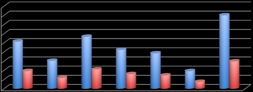
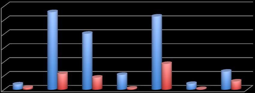
Figure 4 indicates Australia’s export and import volumes which will result from linking with
different schemes and its own domestic ETS. In all cases, Australia’s exports and imports are
reduced. When the ETS results in the contraction of the Australian economy, it will lower
demand for inputs, thus reducing its imports. At the same time, the ETSs are also
19!
!implemented in the other economies and present unfavourable effects on their production and
economies; they will also lower their demands. In this study, the selected economies are the
biggest importers for Australia’s commodities6, hence the reductions in their demand for
inputs would considerably affect the exports from Australia. As a result, Australia’s exports
will fall.
Similar to other macroeconomic findings, if Australia implemented its own domestic ETS,
the effects on their exports and imports would be worst relative to linking with any other
schemes. Linking with India’s scheme is still the best option for Australia in order to lower
unfavourable effects on its exports and imports. In the linkage with India’s scheme,
Australia’s exports and imports only reduce by 1.22% and 1.64%, respectively.
Figure 4: Australia’ export and import volumes from bilateral ETS linkages and its own
domestic ETS
European&
South&Korea& China& Union& United&States& Japan& India& Domestic&ETS&
0%!
B1%!
B2%!
B3%!
B4%!
B5%!
B6%!
B7%!
B8%!
Exports! Imports!
Source: Model simulations.
Figure 5 outlines the prices of electricity and energy in Australia under different scenarios. In
Australia, electricity generation mainly relies on fossil fuels, hence the carbon price
significantly increases the outlay of such a sector, eventually increasing the price of
electricity. The costs of the ETS on the emissions considerably affect the energy sectors, thus
reducing their supplies. In the demand side, although demands for energy by other sectors are
reduced, it would not be adequate to compensate the reductions in the supply of energy. In
!!!!!!!!!!!!!!!!!!!!!!!!!!!!!!!!!!!!!!!!!!!!!!!!!!!!!!!!
6
In the database, total export value at market prices from Australia to these six economies accounts for 68% of
total Australia’ exports.
20!
!addition, an increase in the electricity price also constitutes of an increase in the price of
energy. Taken together, the price of energy subsequently declines. The price of electricity is
particularly high (an increase of 40%) when Australia does not link its ETS with other
schemes. In the case of linking ETSs, the highest increasing rate in the electricity price in
Australia is only at 28.32% with a link with EU-ETS, while its price of electricity only
increases by 9.6% in the case of linking with India’s scheme.
Figure 5: Prices of electricity and energy in Australia in different scenarios
45%!
40%!
35%!
30%!
25%!
20%!
15%!
10%!
5%!
0%!
South! China! European! United! Japan! India! Domestic!
Korea! Union! States! ETS!
Price!of!electricity! Price!of!energy!!
Source: Model simulations.
In Figure 6, we provide the effects of the ETSs on the production levels of the energy sectors
in Australia. The Australian electricity generation sector experiences the highest reduction in
its production level because it is the highest emissions intensive sector. Another negative
effect on the electricity generation sector is the reduction in electricity demand because of
considerable increases in the price of electricity. Production level reductions in coal, gas and
oil products manufacturing sectors are due to considerable reductions in demands from other
sectors and final users, as they are high emissions intensive inputs. Overall reductions in
exports also reduce demands for these energy commodities. In addition, such sectors also
bear the costs on their fugitive emissions.
21!
!Figure 6: Effects of ETSs on production levels of the Australian energy sector in each
scenario
European! Domestic!
South!Korea! China! Union! United!States! Japan! India! ETS!
2%!
0%!
B2%!
B4%!
B6%!
B8%!
B10%!
B12%!
B14%!
B16%!
B18%!
B20%!
B22%!
B24%!
B26%!
B28%!
B30%!
B32%!
B34%!
Coal!mining! Oil!extraction! Gas!extraction!
Oil!products!manufacturing!! Electricity!generation!
Source: Model simulations.
Our findings indicate that subject to the 2030 emissions targets, Australia has the highest
MAC (indicated by the price for permits in Table 3), followed by the European Union, South
Korea, United States, Japan, China and India. China and India have very low MACs
compared to other economies as they have low costs of labour and capital than those other
selected economies. On the other hand, developed countries normally have high costs of
labour and capital, hence for every unit of additional emissions abated, such countries have to
pay relatively higher MACs. As a result, Australia could obtain the optimal net economic
gain by linking its ETS with India. China would be the second choice for Australia to seek
for co-operation in trading emissions. Linking with the European Union or South Korea is a
very costly option for Australia but it is still better than operating its own domestic ETS. The
findings also suggest that the price levels for permits significantly affect the economies. The
higher the price for permits the higher level of unfavourable effects the country has to face.
22!
!6 Conclusions
This paper explores the theory of marginal abatement cost in the case of linking two domestic
ETSs. The purpose behind this is to examine which conditions are critical to obtaining net
economic gain for a country. The findings suggest that if a country has a high MAC, it should
link its domestic ETS with a scheme which has either low MAC or a low emissions reduction
target, in order to maximise its economic benefits from the linkage compared with its
domestic ETS. On the other hand, if a country has a low MAC, it would seek a partner, which
has either high MAC or a high emissions reduction target.
By using the extended GTAP-E model, we can find which economies among the European
Union, United States, China, Japan, South Korea and India, are the most advantageous
partners for Australia with which to bilaterally link its ETS. The findings suggest that subject
to the 2030 emissions targets, Australia has a high MAC while India has the lowest MAC
relative to those for other economies, hence linking ETSs between Australia and India would
yield the highest economic benefits to Australia. China is the second best choice for Australia
to link its ETS, while the most expensive option for Australia is the linkage with the
European Union. However the theoretical framework and simulation results have shown that
linking with any other scheme would always yield better outcomes for Australia than having
its own domestic scheme.
In reality, there are only a few ETSs currently under operation around the world. It is
therefore very challenging for a country to seek an appropriate partner with which to link its
ETS. In addition, country A may be the best partner for country B but country B would not
necessarily be the best partner for country A. However our findings suggest that when there
are many ETSs and each scheme looks for a partner, they will eventually lead to a global
ETS. Consequently, all economies in the linkages are better off as the more schemes in the
linkage, the lower total costs of abatements they would achieve.
23!
!References
Adams, P. D. (2007). Insurance against catastrophic climate change: how much will an
emissions trading scheme cost Australia? Australian Economic Review, 40(4), 432-460.
Adams, P. D., Parmenter, B. R., & Verikios, G. (2014). An Emissions Trading Scheme for
Australia: National and Regional Impacts. Economic Record, 90(290), 316-344.
Arup, T. (2015). Paris UN climate conference 2015: Australia ranked third to last for
emissions. The Sydney Morning Herald. Retrieved from
http://www.smh.com.au/environment/un-climate-conference/paris-un-climate-conference-
2015-australia-ranked-third-to-last-for-emissions-20151207-glhtxf.html
Australian Treasury. (2011). Strong growth, low pollution: modelling a carbon price.
Australian Government, Canberra.
Babiker, M., Reilly, J., & Viguier, L. (2004). Is international emissions trading always
beneficial? The Energy Journal, 33-56.
Babiker, M. H., Criqui, P., Ellerman, A. D., Reilly, J. M., & Viguier, L. L. (2003). Assessing
the impact of carbon tax differentiation in the European Union. Environmental Modeling
& Assessment, 8(3), 187-197.
Bhagwati, J. (1958). Immiserizing growth: a geometrical note. The Review of Economic
Studies, 25(3), 201-205.
Böhringer, C. (2002). Industry-level emission trading between power producers in the EU.
Applied Economics, 34(4), 523-533.
Deparment of Climate Change and Energy Efficiency. (2012). Interim partial (one-way) link
between the Australian emissions trading scheme and the European Union emissions
trading scheme. Retrieved from https://ris.govspace.gov.au/.../04-Linking-EU-ETS-RIS-
for-Publishing-20120830.doc.
Department of Climate Change. (2013). National Greenhouse Gas Inventory - Kyoto
Protocol classifications. Retrieved from http://ageis.climatechange.gov.au/.
Edwards, T. H., & Hutton, J. P. (2001). Allocation of carbon permits within a country: a
general equilibrium analysis of the United Kingdom. Energy Economics, 23(4), 371-386.
European Commission. (2016). International Carbon Market. Retrieved from
http://ec.europa.eu/clima/policies/ets/linking/index_en.htm.
Flachsland, C., Marschinski, R., & Edenhofer, O. (2009). To link or not to link: benefits and
disadvantages of linking cap-and-trade systems. Climate Policy, 9(4), 358-372.
Gerardi, W., & Demaria, A. (2008). Impacts of the carbon pollution reduction scheme on
Australia's electricity markets. Retrieved from
http://lowpollutionfuture.treasury.gov.au/consultants_report/downloads/Electricity_Sector
_Modelling_Report_updated.pdf
Hawkins, S., & Jegou, I. (2014). Linking emission trading schemes. Considerations and
recommendations for a joint EU–Korean carbon market. International Centre for Trade
and Sustainable Development.
Hoque, S., Dwyer, L., Forsyth, P., Spurr, R., Ho, T., & Pambudi, D. (2010). Economic
impacts of greenhouse gas reduction policies on the Australian tourism industry: A
dynamic CGE analysis: CRC for Sustainable Tourism Pty Limited.
Jaffe, J., & Stavins, R. N. (2008). Linkage of tradable permit systems in international climate
policy architecture. National Bureau of Economic Research.
Kemfert, C., Kohlhaas, M., Truong, T., & Protsenko, A. (2006). The environmental and
economic effects of European emissions trading. Climate Policy, 6(4), 441-455.
Kim, K. S., Tang, J. C., & Lefevre, T. (2004). Analysis on Dual System (Carbon Tax plus
Emission Trading) in Domestic CO2 Abatement Strategy-CGE Analysis for Korean Case.
Journal of economic research, 9(2), 271-308.
24!
!Lipsey, R. G., & Lancaster, K. (1956). The general theory of second best. The Review of
Economic Studies, 24(1), 11-32.
McDougall, R., & Golub, A. (2007). GTAP-E: A revised energy-environmental version of
the GTAP model. GTAP Resource, 2959.
Parliament of Australia. (2013a). Chapter 1: Introduction and conduct of the inquiry.
Retrieved from
http://www.aph.gov.au/Parliamentary_Business/Committees/Senate/Economics/Complete
d_inquiries/2010-13/cleanenergypackageinternationalemissionstrading2012/report/c01.
Parliament of Australia. (2013b). Emissions trading schemes around the world. Retrieved
from
http://www.aph.gov.au/About_Parliament/Parliamentary_Departments/Parliamentary_Lib
rary/pubs/BN/2012-2013/EmissionsTradingSchemes.
Ranson, M., & Stavins, R. N. (2015). Linkage of greenhouse gas emissions trading systems:
Learning from experience. Climate Policy, 1-17.
Siriwardana, M. (2015). Australia's new Free Trade Agreements with Japan and South Korea:
Potential Economic and Environmental Impacts. Journal of Economic Integration, 30(4),
616-643.
Tuerk, A. (2009). Linking emissions trading schemes: Routledge.
25!
!You can also read