TTC'2019 The MEEDUSE solution - Transformation Tool Contest
←
→
Page content transcription
If your browser does not render page correctly, please read the page content below
TTC’2019
                                   The MEEDUSE solution

                       Akram Idani1                German Vega1                Michael Leuschel2
                  1
                      Univ. Grenoble Alpes, Grenoble INP, CNRS, LIG. F-38000 Grenoble France
                                       {Akram.Idani, Germa.Vega}@imag.fr

                                        2
                                            Universittsstrae 1n. D-40225 Dsseldorf
                                            Michael.Leuschel@uni-duesseldorf.de

                                                        Abstract
                        The TTC’2019 case study deals with a realistic model transformation
                        which is that of generating binary decision diagrams from truth tables.
                        Among other challenges, the contest emphasizes on correctness which
                        motivated us to apply Meeduse, a tool that we developed in order to
                        define formal semantics with animation facilities of Domain Specific
                        Languages (DSLs). This study allowed us to try how far we can push
                        the abilities of a formal method to be integrated within model-driven
                        engineering. The results were positive and concluding, and show that
                        Meeduse can be adapted to model-transformation which brings to this
                        field formal automated reasoning tools like AtelierB for theorem proving
                        and ProB for model-checking. Meeduse, combined with ProB, provides
                        three strategies: random animation, interactive animation and model-
                        checking. The first strategy runs randomly the transformation rules
                        until it consumes all the truth table rows and then automatically pro-
                        duces the binary decision diagram. The second strategy allows a step-
                        by-step debugging of the transformation rules. And the third strategy
                        is useful for analysing the reachability of some defined states which al-
                        lows to verify whether unwanted situations may happen or not. The
                        proposed solution and demonstration videos can be found at:

                                 https://github.com/meeduse/Meeduse_TTC_2019

1    Introduction
This paper presents the application of Meeduse to the TTC’2019 case study. First we notice that the tool was
conceived in order to define proved executional semantics of domain specific languages (DSLs) by integrating
the formal B method [1] within EMF-based frameworks like XText, Sirius, GMF... Meeduse was recently

Copyright c by the paper’s authors. Copying permitted for private and academic purposes.
In: A. Editor, B. Coeditor (eds.): Proceedings of the XYZ Workshop, Location, Country, DD-MMM-YYYY, published at
http://ceur-ws.org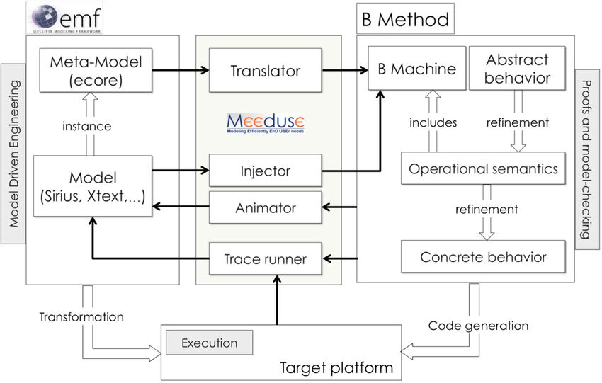
developed (in 2018) and has had successful applications in the safety-critical domain, especially for railway
systems modeling. The reader can refer to [2] for more information about the overall approach of Meeduse.
   The challenge of the TTC’2019 case study for us, is to define and run model transformations as exectu-
tional semantics using a well established formal technique, the B method. This works starts from the following
observations:

    • We are not experts in circuit design and hence the application is limited to the cases provided in the
      TTC’2019 call for solutions. However, we provide transformation rules written in a formal language which
      is assisted by automated reasoning tools; and then we believe that domain experts may be attracted by our
      solution. Indeed, translating a truth table into a binary decision diagram, has several applications in safety
      critical systems where formal methods became a strong requirement.

    • Our objective is not to search for the most compact BDD, but to show how a formal method assisted by
      theorem proving and model-checking techniques can be applied for the particular field of model transfor-
      mation. We note that we discovered too late the update of the TTC call. So, we decided to keep our work
      unchanged and present it as applied to the original BDD meta-model.

    • We have skills in both formal methods (FM) and model-driven engineering (MDE) and we advocate for
      collaborations between both communities in order to take benefits of their complementarities. The Meeduse
      tool favors this communication since it makes possible the use of MDE and FM tools together in one unified
      framework.

2     Brief overview of Meeduse architecture
The goal of Meeduse1 is to support a pragmatic approach to associate model-driven engineering with a proof-
based formal approach. In practice, the tool brings together three technological spaces: EMF for model driven
engineering, B Method [1] for proofs and refinements, and finally the execution of the target system.

                                                        Figure 1: Overview
   Figure 1 depicts the high level architecture of Meeduse, and shows the interactions of the main components
of the tool: Translator, Injector, Animator and Trace runner.

(1) Translator: this component automatically translates an Ecore meta-model into an equivalent B specification
    which represents the structure of the meta-model as well as basic operations like constructors, destructors,
    getters and setters. The resulting B specification can be manually refined by additional invariants and
    concrete operational semantics, as sketched in the right hand side of figure 1. The proof of correction of the
    full specification can be performed with the help of an automatic prover, like the ones proposed by AtelierB.
    1 Meeduse:   Modeling Efficiently EnD USEr needs.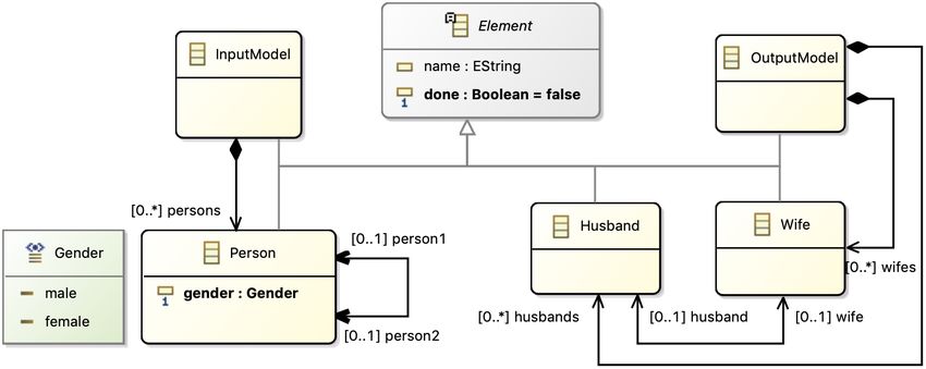
(2) Injector: this component takes a model conforming to the meta-model (which can be designed using EMF-
    based modeling tools like Sirius, GMF, XText, etc) an translate it into a specialized B machine derived from
    the B specification produced from the meta-model. This translation essentially transforms abstract sets
    of the specification (that represent classes in the meta-model) into enumerations representing the concrete
    instances of the model, and hence allows valuations of the B machine variables and model checking over
    finite domains.

(3) Animator: in Meeduse, animation of B specifications is done using the ProB tool [3] which is an open-source
    model-checker supporting the B method. Component Animator asks ProB to animate B operations and gets
    the reached state by means of B variables valuations. Then, the Animator translates back these valuations
    to the initial EMF model resulting in automatic synchronization of the model.

(4) Trace runner: this component allows to play a sequence of operations issued from an execution trace by
    animating the corresponding B operations which leads to automatic modifications of the model. Thanks to
    this component, animation can be done from outside EMF by an external agent running in the execution
    target platform. The trace runner can be useful for conformance validation between the model and the
    execution, and also for some forms of run-time verification.

   Our main objective for the TTC’2019 challenge is to write the model-to-model transformation rules using B
specifications and then to reuse some selected components of Meeduse in order to animate these specifications
given an input model. As Meeduse was not initially designed to define model transformation rules, but to define
DSL execution semantics, we need to rethink the model transformation problem in terms of operational semantics
of an abstract machine.

   The global strategy consists in reusing the Translator component of Meeduse to help automate part of the
writing of the B Machine formal specification of the transformation, use the ProB model checker to animate
the execution of the transformation, and finally reuse the Meeduse’s Animator synchronization capabilities to
obtain the resulting EMF output model. For the TTC’2019 case study, the B specification of a model-to-model
transformation will be structured in two modules:

    • The “Model construction” machine (called B Machine in figure 1) is automatically generated by Meeduse
      from the input and output meta-models of the transformation, and defines basic modeling operations.

    • The “operational semantics” machine is used to manually specify the model-to-model transformation rules
      (notice in the right hand part of figure 1 that Meeduse extensively use the refinement capabilities of the B
      method, we do not exploit this technique for this case study).

   The following section will further describe these two machines and explain the approach in detail, using a
simple transformation for illustration purposes. After that, we will present the complete specification of the
transformation rules of the TTC’2019 case study.

3     A step-by-step overview of Meeduse approach

Presenting the full B formalization of the TTC’2019 case study requires introducing many concepts and prop-
erties, which would be inconvenient for readers from the MDE community who may not be familiar with formal
methods, and particularly with the B method notation. Hence, we decided to introduce in this section our ap-
proach and its underlying formal concepts as a step by step tutorial that uses a simplistic model transformation
example inspired by some basic MDE material available on-line. Application of Meeduse to the TTC’2019 case
study follows similar ideas and will be presented in section 3.
   Figure 2 shows the input and output meta-models for the example transformation. The input of the transfor-
mation is a model defining persons (of any gender) which may be married (represented by the person1/person2
relation) and the output is a model focused only on married wives and husbands (represented as instances of
their respective classes).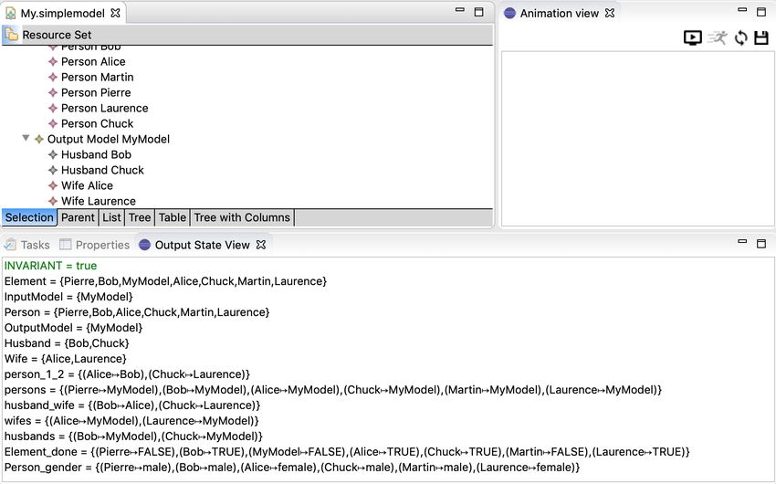
Figure 2: Input/Output meta-models

3.1   Step 1: merging meta-models
As discussed previously, the input of our tool is the meta-model of a DSL, for which we define, using the formal
B method, its execution semantics. In our approach, meta-modeling elements like classes and associations,
which are abstract concepts, are automatically translated into state variables of the corresponding B machine.
Furthermore, constraints defined in the meta-model (for example, the cardinality of attributes) are translated as
invariants of the B specification. The resulting formal specifications allow the specification of the DSL execution
semantics by using B operations. The details of this automatic translation are given in the following section.

   In order to apply the Meeduse approach for model-to-model transformation, our idea is first to merge both
input and output meta-models into a single one which is automatically translated by Meeduse into B, and then
specify the transformation rules as operations of the corresponding B machine. Intuitively, the state of the
transformation execution includes the input model, the partially generated output model and any additional
information required by transformation rules (for instance, traceability links created by other rules).

                                         Figure 3: Merging meta-models

   To concretely illustrate this idea, figure 3 shows the merging meta-model for our simple transformation. Then,
we suggest that the execution semantics of the transformation follows a consumption/production technique:
instances of output classes are created while consuming instances of input classes. In order to keep track of the
modeling elements that have been processed by the transformation, we introduce an abstract meta-class Element
which allows to gather modeling elements consumed by the transformation. This class introduces an attribute
name to identify processed elements and a boolean attribute done which marks consumed input elements. Having
defined this merging meta-model, we are ready to start thinking about the formalization of the transformation.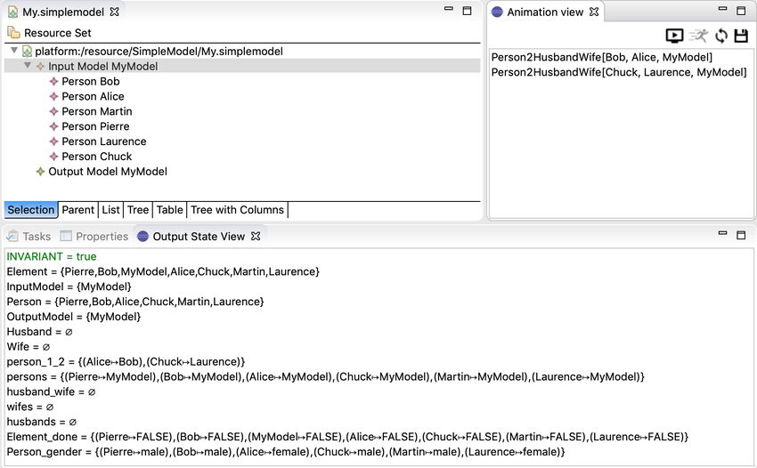
3.2   Step 2: generation of the “model construction” specification
From the merging meta-model, Meeduse automatically generates B specifications that gathers modeling opera-
tions as well as structural invariants. This technique allows to write the transformation rules in the B language.
Figure 4 presents the structural part of the resulting B machine.

                             Figure 4: Structural part of the modeling specification

   In this simple example, we can easily remark that there is a direct correspondence between entities in the meta-
model and declarations in the generated specification. The Meeduse rules for translating an ecore meta-model
into a B specification can be roughly summarized as following:

  • Primitive types (e.g. integer, boolean) become B basic types (Z, BOOL,. . . ).
  • Enumerations and DataTypes are translated into given abstract sets (e.g. Gender={male,female}).
  • For each meta-class there is a variable in the specification (named as the class) representing the set of existing
    instances (e.g. variable Person represents the set of existing instances of class Person). If a class A is a
    subclass of a class B then Meeduse generates an inclusion relationship between their corresponding existing
    instances (A ⊆ B). For example, we get predicate Person ⊆ Element because class Person is a sub-class
    of class Element. The additional class Element introduced in the merging meta-model is translated into an
    abstract set that represents all possible instances. In this example it is designated by set ELEMENT.
  • Each attribute leads to the definition of a variable that is typed as a function from the set of possible
    instances to the attribute type (e.g. Person gender ∈ Person → gender ). The function specializations
    depend on multiplicities and the optional/mandatory character of the attribute. For example, attribute
    done in class Element is an optional boolean attribute, then the corresponding variable is a partial function
    defined as: Element done ∈ Element →  7 BOOL.
  • References are also represented as functional relations between the sets of possible instances issued from both
    source and target classes (e.g. husband wife ∈ Husband   7 Wife). Like attributes, the relation specializations
    depend on the reference cardinalities (and its opposite) like for example, the husband wife variable which is
    a partial injection.

   The behavioral part of the generated B machine provides all basic operations for model manipulation: getters,
setters, constructors and destructors; for this reason we often refer to this machine as the “model construction”
machine. Figure 5 shows the specification of two generated operations. Operation Husband NEW is a constructor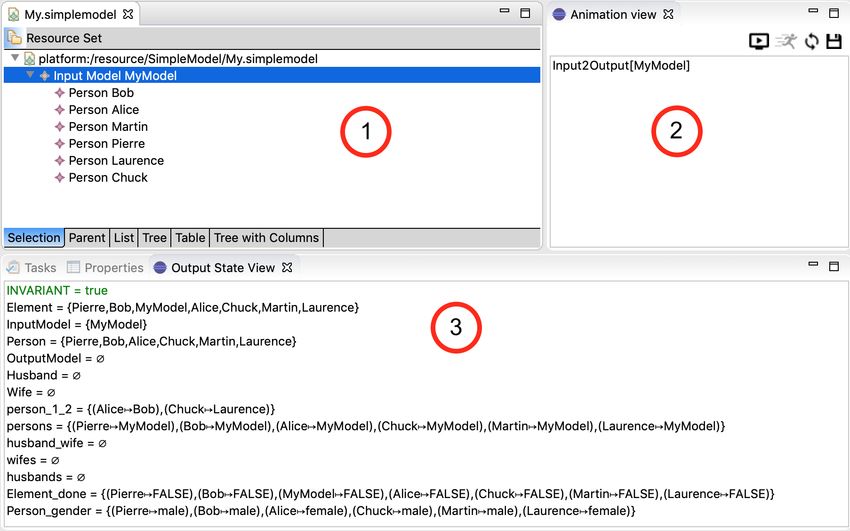
that creates an instance of class Husband. This operation takes an element from the possible objects defined by
abstract set ELEMENT and adds it to the set of existing instances of class Husband. Operation Husband SetWife
is a setter that straightforwardly assigns a value to the bi-directional reference husband/wife.

      Husband NEW (aHusband ) =                       Husband SetWife (aHusband,aWife) =
      PRE                                             PRE
        aHusband ∈ ELEMENT                              aHusband ∈ Husband
      THEN                                              ∧ aWife ∈ Wife
        Husband := Husband ∪ {aHusband } k            THEN
        Element:= Element ∪ {aHusband }                 husband wife(aHusband ) := aWife
      END;                                            END;

                         Figure 5: Generated constructor and setter for class Husband

   Notice that this step is analogous to what happens in MDE tools that generate code from meta-models. For
instance, from a given meta-model definition EMF can generate Java modeling code (getters, setters, etc), that
can be used to program model transformation in Java. In the same way, Meeduse generates a B machine that
can in turn be used to specify model transformations in B.
   The B specification issued from our simple meta-model is about 335 lines of code with 34 basic operations
which are proved correct (with respect to the structural invariant) by construction. Proofs were carried out using
AtelierB, for this simple specification it generated 120 proof obligations, which were all automatically proved by
the theorem prover. This means that the use of these modeling operations guarantees the preservation of the
structural properties (invariant) of the meta-model. They will never create an invalid instance contrary to a java
based technique like that of EMF or other tools.

3.3   step 3: writing the transformation rules
A model transformation is manually written in a new B machine as a set of B operations that can reuse the
modeling operations defined in the simpleModel machine (figures 4 and 5). Each transformation rule is defined
as a B operation composed of two parts: the guard and the action. The guard gives the conditions under which
the rule can be triggered, and the action specifies a sequence of calls to modeling operations (from machine
simpleModel) whose effect is to create the output model.

                                            Person2HusbandWife =
                                              ANY output, p1, p2 WHERE
                                                  output ∈ OutputModel
                                                  ∧ p1 ∈ Person ∧ p2 ∈ Person
                                                  ∧ Person gender(p1) = male
                                                  ∧ Person gender(p2) = female
  Input2Output =                                  ∧ ((p1 7→ p2) ∈ person 1 2 ∨ (p2 7→ p1) ∈ person 1 2)
     ANY input WHERE                              ∧ Element done[{p1, p2}] = {FALSE}
       input ∈ InputModel                         ∧ (husbands ∪ wifes)[{p1,p2}] = ∅
        ∧ input 6∈ OutputModel                THEN
     THEN                                        Husband NEW(p1) ;
       OutputModel NEW(input)                    Wife NEW(p2) ;
     END;                                        Husband SetWife(p1, p2) ;
                                                 OutputModel AddHusbands(output, p1) ;
                                                 OutputModel AddWifes(output, p2) ;
                                                 Element SetDone(p1, TRUE) ;
                                                 Element SetDone(p2, TRUE)
                                              END
                                            END

                                  Figure 6: Transformation rules written in B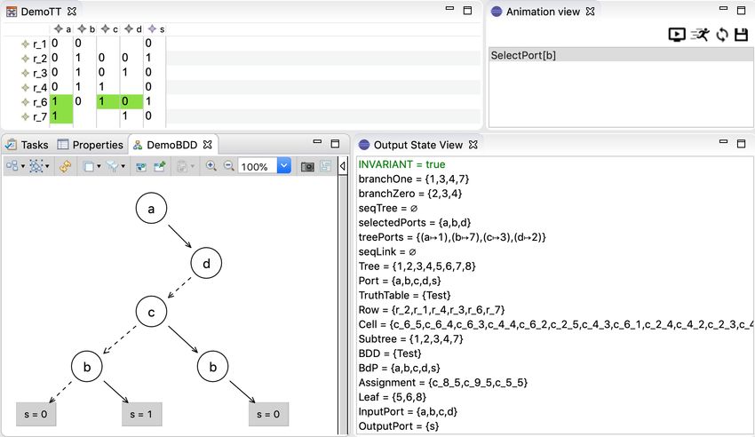
For our simple example, we defined the following two transformation rules (detailed in figure 6):
• Operation Input2Output creates an OutputModel for each InputModel. It takes any existing instance
of class InputModel (input ∈ InputM odel) which has not been yet transformed (condition input 6∈
OutputM odel) and then its action creates the new instance of OutputModel by calling basic operation
OutputModel NEW(input).
• Operation Person2HusbandWife takes two instances of class Person representing a married couple (defined
by parameters p1 and p2) and translates them into instances of classes Husband and Wife in the resulting
output model. The enabling conditions for this transformation rule are:
– there exists an output model (output ∈ OutputM odel)
– the input instances satisfy a pattern, p1 is a male (Person gender(p1) = male), p2 is a female (Per-
son gender(p2) = female) and they are married ((p1 7→ p2) ∈ person 1 2 ∨ (p2 7→ p1) ∈ person 1 2)
– The input instances have not been already processed by a previous execution of the transformation
(Element done[{p1, p2}] = {FALSE} and (husbands ∪ wif es)[{p1, p2}] = ∅)
We can remark that the chosen style for specifying the transformation rules in B reminds transformation
languages available in the MDE community. The specification of the rule guard (clause ANY) is similar to some
declarative transformation languages (it looks like the where condition and checkonly patterns in QVT relational
for example). Nonetheless, the action part has a more imperative style. As B is not a specialized language for
model transformation, some aspects have to be taken care explicitly, for instance we have to check that a rule is
not applied several times for the same input.
An important aspect that is worth mentioning is that we do not specify explicitly the execution order of the
rules. The semantics of a B machine is that, at any given point during the execution, the system considers all
enabled operations and makes a non-deterministic choice. The choice of the parameters in the ANY clause is
also non-deterministic, meaning that at any execution state, the system will select any objects that satisfy the
condition and use them as arguments for the operation.
However, in this example we have indirectly prescribed an order of execution, because in the guard of the
Person2HusbandWife rule we check for the existence of an object created by the Input2Output rule. This
strategy is also similar to some declarative transformation languages that use traceability information to infer
an execution order. The dynamics of a B machine execution will be further explored in the following sections.
A final point concerns the correctness of the transformation rules. As mentioned in the previous section, the
individual model construction operations (constructors, setters, . . . ) were proved correct, then the result of exe-
cuting a sequence of operations in the action part of a rule will obviously preserve the model structural properties.
However, we also need to prove that the order of the sequence of calls is correct, meaning that the preconditions
of every operation in the sequence are satisfied. Lets’s consider for example operation Husband SetWife which
can be applied only on existing instances of classes Husband and Wife: aHusband ∈ Husband ∧ aWife ∈ Wife.
As actions Husband NEW and Wife NEW produce these instances, then the proof of correctness associated to the
call of Husband SetWife in rule Person2HusbandWife succeeds.
For our example rules, the AtelierB generated 13 additional proof obligations, which were automatically
proved. This means that we don’t need to test the validity of the input models or verify the output model using
the EMF validator.
3.4 step 4: animation and debugging
Proofs are mainly for a verification purposes (i.e. “do the transformation right?”). However, we need to validate
the rules in order to be sure that they produce the results expected by a domain expert (i.e. “do the right
transformation?”). For this purpose, Meeduse provides an interactive animation facility that uses the ProB [3]
animator in background.
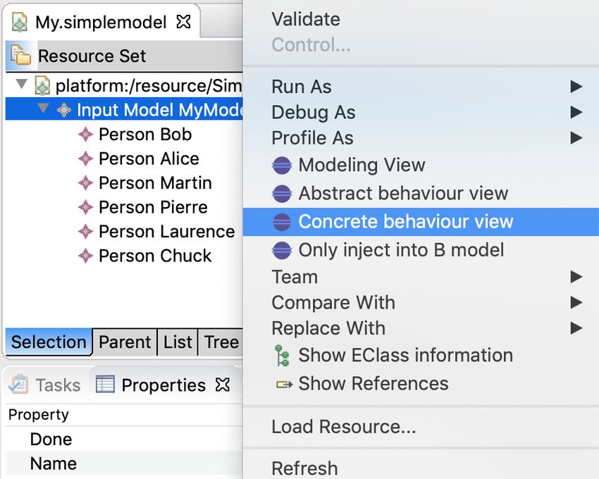
In Meeduse the user can load an EMF input model and injects it in the B specifications as variable valuations.
Figure 7 shows an example input model open in the EMF editor, the model represents a group of 6 people. The
figure also shows how to invoke this functionality in the tool: right click on the root element of a model and then,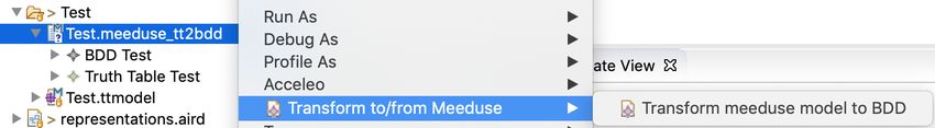
choose Concrete behaviour view. After loading the model, Meeduse asks ProB to animate the initialization
and then gets the initial state of the machine. Given this state, ProB computes the list of operations whose
guards are satisfied and which can then be animated from the initial state. Figure 8 is a screen-shot of Meeduse
after loading the example input model.

                                     Figure 7: Loading a model in Meeduse

   At this point we can make some observations for our example. From the input model (loaded in the EMF
editor in view 1 of figure 8) Meeduse initialized some of the variables of the machine and asked ProB to calculate
the initial state of the machine. The state of the machine is displayed in View 3 of figure 8 (called Output State
View). In particular, we can observe that the variables that represent classes of the input model (InputModel,
Person) and those of the output model (OutputModel, Husband and Wife) were initialized as follows:
      InputModel := {MyModel} ||
      Person := {Bob, Alice, Martin, Pierre, Laurence, Chuck} ||
      OutputModel := {} ||
      Husband := {} ||
      Wife := {} ||
   Notice that the Output State View not only shows the valuations of the variables, but also detects invariant
violations (a facility provided by ProB for a given valuation). If the input model contains errors, this view will
detect them. This invariant validation acts like the EMF validator: the model is validated against its meta-model.
In B, we say that the valuations satisfy the invariant.
   Meeduse also asked ProB to calculate the list of operations that are enabled in the current state. This list
of operations is shown in view 2 of figure 8 (the animation view). ProB not only calculates the enabled
operations, but also their arguments values when their guards are satisfied. In the case that there are several
combinations of values that satisfy an operation guard, Meeduse proposes all the combinations in the animation
view. In our case, the only enabled operation that can be animated at the initial state is Input2Output, and
applied to parameter MyModel.
   If the user double clicks on this operation Meeduse will ask ProB to animate it, which computes on the one
hand the next reached state and on the other hand the list of operations that are enabled from this new state.
Then Meeduse gets the reached state and translates it back to the EMF model. Figure 9 is a screen-shot after
animation of operation Input2Output from which we can observe the effect of the rule execution.
   The output state view shows the new variable valuations computed by ProB, in particular we can observe
that variable OutputModel contains a new element. The EMF modeling editor is automatically synchronized.
An instance of class Output, named MyModel was created, which is the expected result of rule Input2Output.
And finally, the animation view shows that from this new state only operation Person2HusbandWife can be
triggered, but with two possible parameter valuations: Bob,Alice,MyModel and Chuck,Laurence,MyModel. The
user can then choose which one to animate.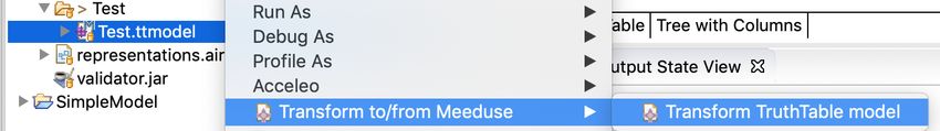
Figure 8: Meeduse screenshot: initial values

                          Figure 9: Meeduse screenshot: after animation of rule 1

  This interactive animation technique applies the transformation rules step-by-step to the input EMF model
which is useful for debugging. The animation stops when the B specification reaches a deadlock: a state from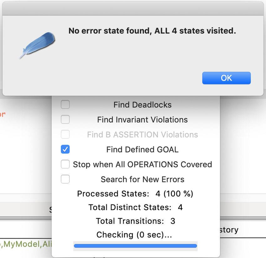
which there is no other possible operation to animate. It also stops when an invariant violation is detected,
which is not possible in our case as we entirely proved using AtelierB that the transformation rules preserve the
invariant. Figure 10 gives the result of the animation at the final state. In the output model, two husbands (Bob
and Chuck) and two wives (Alice and Laurence) were created, with the corresponding marriage relation. The
valuations of the B variables showed in the output state view are equivalent to the EMF model since Meeduse
maintains this equivalence at every animation step.

                          Figure 10: Meeduse screenshot: after animation of all rules

   When the domain expert agrees with the behaviors showed by animation, transformation rules can be played
without any human interaction. After loading a model (figure 7) the user can enable the automatic runner from
the animation view by clicking on the corresponding icon. This runner executes a random animation: at every
step it chooses randomly an operation from those provided by ProB and automatically animates it until reaching
the ending state where a deadlock or an invariant violation is detected.

3.5   step 5: Proving the transformation
Application of a formal method to model transformation brings several benefits to this field. Indeed, since
Meeduse produces a formal specification and automatically manages the traceability between EMF models and
the B machine valuations, we can go a step further towards the usage of automatic reasoning tools like model-
checkers.
   The invariants discussed in step 2 define the properties of our meta-model, not those of the transformation.
One way to analyze the transformation and have some confidence about its correctness is to define unwanted
states and ask ProB to find them by model-checking. In the following we present some example goals that we
defined for our simple transformation:

  GOAL1    ==   ∃ pp . (pp ∈ Husband ∧ Person gender(pp) = female) ;
  GOAL2    ==   ∃ pp . (pp ∈ Wife ∧ Person gender(pp) = male) ;
  GOAL3    ==   ∃ (p1, p2).((p1 7→ p2) ∈ husband wife ∧ {p1,p2} 6⊆ dom(person 1 2) ∪ ran(person 1 2)) ;
  GOAL4    ==   Husband ∩ Wife 6= ∅
The three first goals are linkage properties between the input and the output meta-model. Goal1 and Goal2
for example state that an instance of class Husband is created but from a Person whose gender is female and
vice-versa. Goal3 means that a husband and his wife in the output model are created but without any existing
marriage link between the input persons from which they originate. Goal4 represents a forbidden property of
the output meta-model and means that someone is husband and wife at same time.
Given the B specification extracted from the initial model (that of figure 8), we can ask ProB, from outside
Meeduse, to find by model-checking states where one of these goals are satisfied. The answer of ProB is given in
figure 11. It mentions that all state space is explored without finding any of the four goals. Since the state space
is entirely bounded thanks to valuations, ProB is able to compute all reachable states. This model-checking
proof gives a good confidence about the correctness of the transformation. It can be applied to bigger examples
in the limits of space memory and the model-checker capacities.
Figure 11: Result of ProB after model-checking the input model
3.6 Discussion
In this section we used together four tools:
• EMF for meta-modeling and the automatic extraction of an editor plugin in a classical MDE approach. This
was the subject of step 1.
• The AtelierB prover for theorem proving in order to prove that the various B specifications (the model
construction and the model transformation) preserve the meta-model structural properties. This was the
subject of steps 2 and 3.
• ProB for one of its numerous model-checking capabilities (step 5).
• Meeduse was involved in step 2 in order to translate an ecore meta-model into a B specification, and also
in steps 3 and 4 for debugging and executing the transformation given an instance of the input model.
In this work, we are not advising that the MDE expert learns the B method and its associated tooling, or
conversely that the FM expert learns meta-modeling with its tools. We believe that skills in both domains are
required, and we suggest a way to make people collaborate. Meeduse provides practical solutions for that, as
shown by this simplistic example. Furthermore, we didn’t exploit neither the whole MDE capabilities nor the
whole FM capabilities, but we limited our proposal there to a subset of what can be done for the particular case
of model-to-model transformations. Some interesting research directions would be:• MDE: Apply a model-to-text transformation in order to translate the proved B operations into a well-known
MDE language for model-to-model transformation, like ATL. Indeed, once the rules are proved (using a
theorem proving technique, or a bounded model-checking approach), we can think about their translation
into the ATL language (for example) then apply the ATL tool for running the transformation.
• FM: Apply refinement in order to produce a correct implementation from the B specifications. In B, the
refinement technique is well mastered and assisted by automated reasoning tools. It starts from abstract
specifications and incrementally introduces properties with additional data until reaching an implementation
of the transformation rules.
4 Application to the TTC’2019 case study
4.1 Provided artifacts and some technical details
Meeduse is an eclipse plugin, distributed as an update site of the Eclipse Modeling Platform. We developed and
tested it on the Oxygen distribution of Eclipse, with various operating systems: MacOS, Windows and Linux.
Its application to the TTC’2019 case study followed exactly the same principles than those presented in the
previous section and led to several artifacts provided at:
https://github.com/meeduse/Meeduse_TTC_2019
• Meta-modeling artifacts: provided in folder Meeduse TTC 2019/eclipse wksp/Meeduse tt2bdd/model/
– The merging meta-model (named meeduse tt2bdd.ecore) follows the main principles of the merging
step described in section 3.1. This meta-model was done in EMF Ecore-Tools.
– The model construction B specification (named meeduse tt2bdd.mch) was first automatically generated
by Meeduse from the ecore file of the merging meta-model. Then, it was manually enhanced by
few additional utility operations which were useful for the transformation but not yet integrated to
Meeduse. This B specification is about 1162 lines of code. Refer to section 3.2 for an overview of its
main principles.
– Files with extensions .bmethod, .trace and .uml can be exploited by a Meeduse developer. Note
that the tool applies a UML-to-B transformation technique that’s why it first generates a UML model
from the ecore file. It also integrates a meta-model of the B method which is instantiated during the
transformation. The textual file .mch is produced from this instance.
– The model transformation specification (named meeduse tt2bddref.ref). This file will be explained
in the following since it gives our solution rules to the TTC’2019 call. The proposed transformation is
based on five rules: TruthTable2BDD, SelectPort, setLinks, Transform and Continue.
• Merging models driver: provided in folder Meeduse TTC 2019/eclipse wksp/MeeduseRepo/. On the one
hand, this driver produces an instance of the merging meta-model (meeduse tt2bdd.ecore) from a truth
table conforming to TT.ecore. The generated instance contains exactly the same input truth table. On the
other hand, it extracts a binary decision diagram from the merging model which produces an instance of
meta-model BDD.ecore. The generated instance contains exactly the same output BDD than that computed
by Meeduse when executing the transformation rules. This driver is implemented as generic as possible in
order to be reused further for other kinds of meta-models. Figure 12 shows how to use the driver on an
input truth table. Simply right click on your .ttmodel file and then choose Transform to/from Meeduse
-> Transform TruthTable model. It will create a .meeduse tt2bdd file. After running the transformation
right click on the .meeduse tt2bdd file and choose Transform to/from Meeduse -> Transform meeduse
model to BDD. The resulting file is a .bddmodel on which the validator, given by the TTC’2019 organizers,
can be executed.
• Modeling artifacts: provided in folder Meeduse TTC 2019/runtime wksp/
– meeduse.tt2bdd.design: this is a sirius project allowing to have a nice representation of the truth table
and of the BDD. When executed on a given root element of an EMF resource, Meeduse is synchronised
with the resource and then every eclipse tool also synchronised with the same resource is expected
to be compatible with Meeduse. We tested it with: Sirius, XText, Ecore Reflective Editor and alsoFigure 12: Using the merging driver
automatically generated outline editor plugins from .genmodel files. In this solution, one can use our
Sirius artifacts for visualizing the models (the TT and the BDD) issued from the merging meta-model.
Sirius has two benefits: (1) it favours graphical animation because when executed the model changes
(input elements are consumed and output elements are produced) and Sirius automatically updates its
rendering at every modification of the model, and (2) it is an easy-way to define conditional styles which
changes the visual representation depending on some OCL-like conditions. For this example, when a
cell is selected it becomes green which allows the user to know which rows are being transformed.
Figure 13 shows the sirius views of a truth table under transformation and the current state of the
corresponding BDD. In this snapshot some cells of rows r 6 and r 7 are currently selected (for ports
a, c, d), and a sub-part of the BDD is produced from rows already consumed (r 5 and r 8). In our
transformation a consumed row is simply removed from the truth table.
Figure 13: A Truth Table under transformation
– meeduse.tt2bdd.sample: in this folder we provide models with the resulting BDD. Every model is ranged
in a sub-folder with the same name as the model. Folder Test contains the illustration model used in the
TTC’2019 call for solutions. The demo videos are also done based on this model. Each of these folders
contains the three files: .ttmodel, .bddmodel and .meeduse tt2bdd. Note that our (bad) result is that
the biggest model that Meeduse was able to deal with is in folder GeneratedI12O2Seed7634. For the
two remaining models (GeneratedI14O4Seed7634 and GeneratedI15O5Seed282316) ProB produced
a memory overhead. We are currently trying to enhance our tools in order to load such huge models.
However, for the other models, our results were satisfactory since our major interest in the TTC’2019
challenge is not to load the most explosive model but to provide a correct transformation on which
proof of correctness is done thanks to formal automated reasoning tools: we guarantee the preservation
of the meta-model structural properties and also the transformation properties that we identified.4.2 Transformation rules
The transformation rules are specified in file meeduse tt2bddref.ref where the rules are written in ASCII
encoding. In appendix the whole specification (which is about 150 lines of code) is presented using the B
language. In this subsection we describe the general idea of the transformation.
First, the definition clause allows to define some kinds of helpers (we reuse the ATL term) that calculate some
formula based on the set theory and the first order logic predicates:
−1 −1 −1
zeroCells(pp) == (cellPort [{pp}] ∩ cells [selectedRows]) ∩ Cell value [{FALSE}] ;
−1 −1 −1
oneCells(pp) == (cellPort [{pp}] ∩ cells [selectedRows]) ∩ Cell value [{TRUE}] ;
selectedCells == dom(Cell selected B {TRUE}) ;
−1 −1
outputCells(rr) == cells [{rr}] ∩ cellPort [OutputPort] ;
−1 −1
inputCells(rr) == cells [{rr}] ∩ cellPort [InputPort]
• zeroCells applied to a port pp gives all cells with value 0 that belong to the selected rows. The row selection
mechanism will be discussed while presenting the transformation rules. Definition oneCells is similar but
gives cells with value 1.
• outputCells and inputCells applied to a row rr gives the cells that are concerned by an output or an input
port.
• selectedCells gives the set of cells that are consumed during the transformation.
The algorithm proposed in the TTC’2019 call for solutions suggests to find an input port which is (ideally)
defined in all the Rows, and turn it into an inner node. We somehow applied this technique but introduced a
maximality criterion. In fact our algorithm chooses the port whose set of cells is the biggest one, with respect to
the selected rows. This maximality is computed by the following definition called maxPort . Definition maxRow
simply gives the ports of a given row rr.
portRow(rr) == (cellPort −1
; cells) B rr ;
maxPort(pp,rr) == pp ∈ InputPort ∧ rr ⊆ Row ∧
¬ ( ∃ ss . (ss ∈ InputPort ∧ ss 6= pp ∧ ss ∈ dom(portRow(rr))
∧ card(portRow(rr)[{ss}]) > card(portRow(rr)[{pp}]))) ;
4.3 A step-by-by step execution
The screen-shot of figure 14 shows that at the beginning of the transformation the only port that can be selected
is port a. This is the expected result since port a establishes the maximality criterion. Note that in the initial
state all rows are selected and then a has the biggest set of cells in comparison with the other ports.
The Animation view provides two possibilities for selectPort(a) because one can select the zero value or
the one value. The animation of the second occurrence of selectPort(a) leads to figure 15 where cells of value
one of port a are selected and a node is created in the BDD model. In fact, every time a port is selected, a node
in the BDD is created. For this state, formula maxPort identifies port d as the one satisfying the maximality
criterion and then the animation view gives two possible executions of selectPort(d) (for value zero and for
value one).
The animation of the first occurrence of selectPort(d) leads to the model of figure 16 where zero cells of
port d are selected and an other node is created in the BDD model. In this new state four possible rules can be
triggered because ports b and c are equivalent regarding the maximality criterion. Meeduse suggests then two
possibilities for each of selectPort(b) and selectPort(c). Running the second occurrence of selectPort(b)Figure 14: First execution
Figure 15: Second execution
Figure 16: Third execution
Figure 17: Fourth execution
produces figure 17 from which it is possible to trigger finally rule selectPort(c) and hence reach the end of the
selection step with nodes extraction.
From step of figure 17 the execution of the second occurrence of selectPort(c) leads to figure 18 where
only one row r 9 has all its cells selected. Now, only rule Transform(r 9) is proposed. When applied this rule
iterates several times on row r 9 until it transforms it entirely. The first calls transform non-deterministically
the row output cells into assignments with the same values (figure 19). After consuming all output cells (in this
case we have only one output cell), this rule creates a Leaf and then removes the row from the model togetherwith its cells. By this way row r 9 and its cells will not be considered for the next calculus of the enabledness
conditions of the transformation rules.
Figure 18: Fifth execution
Figure 19: Sixth execution
In figure 20, after removing row r 9, the enabled rules are those that create links between nodes, assign-
ments and leafs. These are successive occurrences of operation setLinks: setLinks(1,2), setLinks(2,3),
setLinks(3,4), setLinks(4,5). The valuations correspond to tree identifiers managed by the internal state of
the B specification every time an instance of class tree is produced.
Figure 20: Seventh execution
Figure 21 gives the resulting model after a row is entirely consumed and the corresponding path in the BDD is
produced. Rule continue then updates the internal state of the B machine and makes possible the port selection
process for the remaining rows. From the model of figure 21 only port c with value zero can be selected. Indeed,
given the set of selected rows and cells, only port c satisfies the maximality criterion.
4.4 Checking the transformation rules
The transformation sequence that is executed by Meeduse based on our transformation rules (refer to annexes
for the formal details), can be summarized by:
• TruthTable2BDD: this rule creates a BDD from a truth table under the condition that the BDD was not
previously created. It also creates the BDD input and output ports, and then adds all generated ports to the
BDD. It calls sequentially modeling operations BDD NEW, BddInput NEW, BddOutput NEW and BDD Addports
which were generated from the meta-model.Figure 21: A successive animation of setLink
• SelectPort: this rule selects an input port satisfying the maximality condition and depending on the
current state of the transformation and then decides whether it creates a new tree or reuses a tree already
created. When it creates a tree it calls the modeling operation Subtree NEW. For the first tree only it calls
Tree SetOwnerBDD which marks this first tree as a root tree. These are the first actions that the operation
makes and which are defined by the first SELECT clause. The next actions defined in the second SELECT
clause of this operation select non-deterministically cells of value zero or those of value one. This explains
the two possible instances of operation SelectPort that can be applied to the same selected port.
• Transform: this operation can be triggered only when there is no more one selected row, and allows
to consume the row and its cells. It has two deterministic behaviours defined by clause IF: creates an
assignment for output cells if there exists an output cell not yet consumed, or creates a leaf if all output
cells are consumed.
• Continue: it is not really a transformation rule because it is mainly used as a checkpoint for the model-
checker. The model-checking proof technique applied to this case study, verifies the transformation properties
not for all the state space (like for the tutorial example), but before every call to operation Continue.
The ProB model-checker computes exhaustively all the execution possibilities. Note that we added some
preference to the DEFINITION clause:
SET PREF SHOW EVENTB ANY VALUES == TRUE
SET PREF MAX OPERATIONS == 4
The first preference allows the tool to explicitly show parameters when running the transformation. The
second preference allows to configure the maximum number of enabled operations. In fact, at every step ProB
computes operations whose guard is evaluated to true and will limits its analysis of every operation to the
maximum preferred size. In the example above, number 4 is sufficient but the user can choose to modify it for
his convenience. ProB allows to check the reachability of unwanted states using goals and based on the maximum
number of computed operations:
• For every consumed row, one distinct leaf is created.
• For every output cell of a consumed row, one assignment is created with the same value.
• When there is no row to deal with then all tree links are produced.
• Values of trees in a computed BDD path (before running operation Continue) are equivalent to the selected
cells values in the consumed row.
Our exhaustive model-checking validation technique was done on input models of reasonable sizes: until 5
input ports, 2 output ports, and 32 rows. We believe that the model-checking proofs done given these models
are sufficient to have some confidence about our rules because most of the provided models are generated by a
combinatorial technique. We think that since the proof succeeded for a restricted number of port combinations,
then it can be generalized for bigger combinations. Not only the algorithm applies redundantly the same principles
to the consumed rows but also the properties of these rows (by means of cell values and connexion with ports)
are similar and they don’t change during the transformation.Further study may be required in order to show the existence of a least fixed point, from which one can
generalize the proof and stop building input models for the exhaustive model-checking. For bigger examples we
simply apply Meeduse as a runner of the transformation in order to get the output BDD. For these examples
we set property SET PREF MAX OPERATIONS to one, which forces ProB to compute only one instance of each
operation which is immediately animated by Meeduse in the automatic execution mode. Finally, we note that all
our output models successfully passed the validator provided by the TTC’2019 organizers which was somehow
expected since we spent a lot of time on checking the B specifications using automated reasoning tools. Meeduse
was also helpful for debugging the formal specifications thanks to the visualization designed in Sirius.
5 Conclusion
First, from a methodological point of view we were able to define how formal DSL execution semantics can be
applied to define model transformations. Merging meta-models required the implementation of an additional
driver, but we believe that Meeduse can be adapted to deal with two or several heterogeneous meta-models.
This issue is now considered as a possible evolution of the tool. In general, we are satisfied by the application of
Meeduse to the model-to-model transformation problem because as far as we know none of the existing works
combine theorem proving and model-checking in a publicly available tool and which is well integrated within
EMF-based platforms.
For performance, it mainly depends on the performance of ProB. Execution times spent by the tool to generate
the output models are given in table 1. The number of model elements grow exponentially. For 14 input ports
and 2 output ports, Meeduse reached an out of memory. For bigger examples, it should be useful to try the
experiments on a machine with higher performances than that on which we have done these measures.
Input Model rows input ports output ports Cells Exec. Time
GeneratedI4O2Seed42 16 4 2 96 3s
GeneratedI5O2Seed5 32 5 2 224 5s
GeneratedI8O2Seed68 256 8 2 2560 1mn3s
GeneratedI8O4Seed68 256 8 4 3072 2mn1s
GeneratedI10O2Seed68 1024 10 2 20480 18mn8s
GeneratedI12O2Seed7634 4096 12 2 57344 6h40mn
Table 1: Some performance measures
For readability, we believe that the verbose notation of the B method is accessible because it recalls some
programmatic styles. It is often said to be less difficult than other formal notations. Our transformation file is
about 150 lines which remains reasonable. However, we don’t believe that an MDE expert must become expert
in the B method in order to apply Meeduse. We think that model transformation interests the safety-critical
community whose main intention is to develop systems which are bug-free because a failure can lead to human
loss. This study gives solutions to this problem with the support of a tool. In this sense we advocate for a
collaboration between MDE and FM experts. The B specification that we provide is expected to be readable
for a FM expert, may be more readable than an ATL or a QVT transformation. But this intuition needs some
empirical studies in order to be confirmed.
References
[1] J.-R. Abrial. The B-book: Assigning Programs to Meanings. Cambridge University Press, New York, NY,
USA, 1996.
[2] Akram Idani, Yves Ledru, Abderrahim Ait Wakrime, Rahma Ben Ayed, and Philippe Bon. Towards a
tool-based domain specific approach for railway systems modeling and validation. In Third International
Conference, RSSRail 2019, Lille, France, June 4-6, 2019, Proceedings, volume 11495 of LNCS, pages 23–40.
Springer, 2019.
[3] Michael Leuschel and Michael Butler. Prob: an automated analysis toolset for the b method. International
Journal on Software Tools for Technology Transfer, 10(2):185–203, Mar 2008.Appendix
REFINEMENT
meeduse tt2bddref
REFINES
meeduse tt2bddmain
INCLUDES
meeduse tt2bdd
DEFINITIONS
selectedRows ==
LET cr BE cr = {cc,rr | rr ∈ Row ∧ cc= card(cells −1 [{rr}] ∩ selectedCells)} IN
LET mx BE mx = max(dom(cr)) IN
cr[{mx}]
END
END;
portRow(rr) == (cellPort −1 ; cells) B rr ;
maxPort(pp,rr) == pp ∈ InputPort ∧ rr ⊆ Row ∧
¬ ( ∃ ss . (ss ∈ InputPort ∧ ss 6= pp ∧ ss ∈ dom(portRow(rr))
∧ card(portRow(rr)[{ss}]) > card(portRow(rr)[{pp}]))) ;
zeroCells(pp) == (cellPort −1 [{pp}] ∩ cells −1 [selectedRows]) ∩ Cell value −1 [{FALSE}] ;
oneCells(pp) == (cellPort −1 [{pp}] ∩ cells −1 [selectedRows]) ∩ Cell value −1 [{TRUE}] ;
selectedCells == dom(Cell selected B {TRUE}) ;
outputCells(rr) == cells −1 [{rr}] ∩ cellPort −1 [OutputPort] ;
inputCells(rr) == cells −1 [{rr}] ∩ cellPort −1 [InputPort]
VARIABLES
branchOne, branchZero,
seqTree, selectedPorts, treePorts, seqLink
INVARIANT
branchOne ⊆ Tree ∧
branchZero ⊆ Tree ∧
selectedPorts ⊆ Port ∧
treePorts ∈ InputPort ↔ Tree ∧
seqTree ∈ seq(Tree) ∧
seqLink ∈ seq(BOOL)
INITIALISATION
branchOne, branchZero, selectedPorts := ∅ , ∅ , ∅ ||
treePorts, seqTree, seqLink := ∅ , ∅ , ∅ ||
setLastTree(card(Subtree))
1OPERATIONS
TruthTable2BDD =
ANY src WHERE
src ∈ TruthTable ∧ src 6∈ BDD
THEN
BDD NEW(src) ;
BddInput NEW(InputPort) ;
BddOutput NEW(OutputPort) ;
BDD Addports(bdd, InputPort ∪ OutputPort)
END;
SelectPort =
ANY port WHERE
InputPort 6= ∅
∧ port ∈ BddInput
∧ port 6∈ cellPort[selectedCells]
∧ maxPort(port, selectedRows)
∧ ran(seqTree) ∩ Leaf = ∅
THEN
SELECT
port ∈ selectedPorts
THEN
seqTree := seqTree ← (treePorts(port))
WHEN
port 6∈ selectedPorts
∧ ¬ ( ∃ portBis . (portBis 6∈ cellPort[selectedCells]
∧ maxPort(portBis, selectedRows)
∧ portBis ∈ selectedPorts))
THEN
Subtree NEW(port) ;
BEGIN
selectedPorts := selectedPorts ∪ {port} ||
treePorts(port) := lastTree ||
seqTree := seqTree ← (lastTree)
END ;
IF lastTree = 1 THEN
Tree SetOwnerBDD(lastTree, bddPorts(port))
END
END ;
SELECT zeroCells(port) 6= ∅ THEN
Cells SetSelected(zeroCells(port), TRUE) ||
branchZero := branchZero ∪ treePorts[{port}] ||
seqLink := seqLink ← (FALSE)
WHEN oneCells(port) 6= ∅ THEN
Cells SetSelected(oneCells(port), TRUE) ||
branchOne := branchOne ∪ treePorts[{port}] ||
seqLink := seqLink ← (TRUE)
END
END;
2setLinks =
ANY t1, t2 WHERE
t1 = first(seqTree) ∧ t2 = first(tail(seqTree))
∧ ran(seqTree) ∩ Leaf 6= ∅
∧ card(seqTree) > 1
THEN
IF first(seqLink) = TRUE THEN
Subtree SetTreeForOne(t1, t2) ||
seqLink := tail(seqLink)
ELSE
Subtree SetTreeForZero(t1, t2) ||
seqLink := tail(seqLink)
END ||
seqTree := tail(seqTree)
END;
Continue =
SELECT
card(seqTree) = 1 ∧ ran(seqTree) ∩ Leaf 6= ∅
THEN
seqTree := tail(seqTree)
END ;
Transform =
ANY row WHERE
row ∈ selectedRows
∧ card(selectedRows) = 1
∧ ∀ cc . (cc ∈ cells −1 [{row}] ∧ cellPort(cc) 6∈ OutputPort ⇒ Cell selected(cc) = TRUE)
THEN
IF card(outputCells(row)) > card(assignPort[outputCells(row)]) THEN
ANY as WHERE as ∈ outputCells(row) ∧ as 6∈ Assignment THEN
Assignment NEW(as, cellPort(as), Cell value(as))
END
ELSE
Leaf NEW ;
seqTree := seqTree ← (lastTree) ;
Assignments SetOwner(outputCells(row), lastTree) ;
Cells Free(inputCells(row) ∪ outputCells(row)) ;
selectedPorts := selectedPorts -
{app | app ∈ selectedPorts ∧ treePorts(app) : (branchZero ∩ branchOne)};
Row Free(row)
END
END
END
3You can also read