Characterization of Extreme Wave Conditions for Wave Energy Converter Design and Project Risk Assessment - MDPI
←
→
Page content transcription
If your browser does not render page correctly, please read the page content below
Journal of
           Marine Science
           and Engineering

Article
Characterization of Extreme Wave Conditions for
Wave Energy Converter Design and Project
Risk Assessment
Vincent S. Neary 1, * , Seongho Ahn 1 , Bibiana E. Seng 2 , Mohammad Nabi Allahdadi 3 ,
Taiping Wang 4 , Zhaoqing Yang 4 and Ruoying He 3
 1    Sandia National Laboratories, Water Power Technologies, Albuquerque, NM 87185, USA
 2    Department of Statistics, The Pennsylvania State University, State College, PA 16802, USA
 3    Department of Marine, Earth, and Atmospheric Sciences, North Carolina State University, Raleigh,
      NA 27606, USA
 4    Pacific Northwest National Laboratory, Seattle, WA 98109, USA
 *    Correspondence: vsneary@sandia.gov

 Received: 17 March 2020; Accepted: 15 April 2020; Published: 18 April 2020

 Abstract: Best practices and international standards for determining n-year return period extreme
 wave (sea states) conditions allow wave energy converter designers and project developers the
 option to apply simple univariate or more complex bivariate extreme value analysis methods. The
 present study compares extreme sea state estimates derived from univariate and bivariate methods
 and investigates the performance of spectral wave models for predicting extreme sea states at
 buoy locations within several regional wave climates along the US East and West Coasts. Two
 common third-generation spectral wave models are evaluated, a WAVEWATCH III®model with a
 grid resolution of 4 arc-minutes (6–7 km), and a Simulating WAves Nearshore model, with a coastal
 resolution of 200–300 m. Both models are used to generate multi-year hindcasts, from which extreme
 sea state statistics used for wave conditions characterization can be derived and compared to those
 based on in-situ observations at National Data Buoy Center stations. Comparison of results using
 different univariate and bivariate methods from the same data source indicates reasonable agreement
 on average. Discrepancies are predominantly random. Large discrepancies are common and increase
 with return period. There is a systematic underbias for extreme significant wave heights derived from
 model hindcasts compared to those derived from buoy measurements. This underbias is dependent
 on model spatial resolution. However, simple linear corrections can effectively compensate for this
 bias. A similar approach is not possible for correcting model-derived environmental contours, but
 other methods, e.g., machine learning, should be explored.

 Keywords: extreme significant wave height; wave hindcast; wave energy resource assessment;
 WEC design

1. Introduction
     Best practices for determining the site-specific environmental conditions, design load cases (DLC),
and load responses for maritime structures and their subsystems (e.g., offshore oil platforms, offshore
floating wind turbines, wave energy converters, and mooring systems) are found in a variety of
international standards, e.g., [1–3]. Some of the most common load types experienced by maritime
structures include hydrostatic, hydrodynamic (currents, waves), and aerodynamic (wind) loads. Design
conditions include transport, operation under normal conditions occurring every year, and survival
under extreme or abnormal environmental conditions for a range of return periods (e.g., 1, 5, 50,

J. Mar. Sci. Eng. 2020, 8, 289; doi:10.3390/jmse8040289                             www.mdpi.com/journal/jmse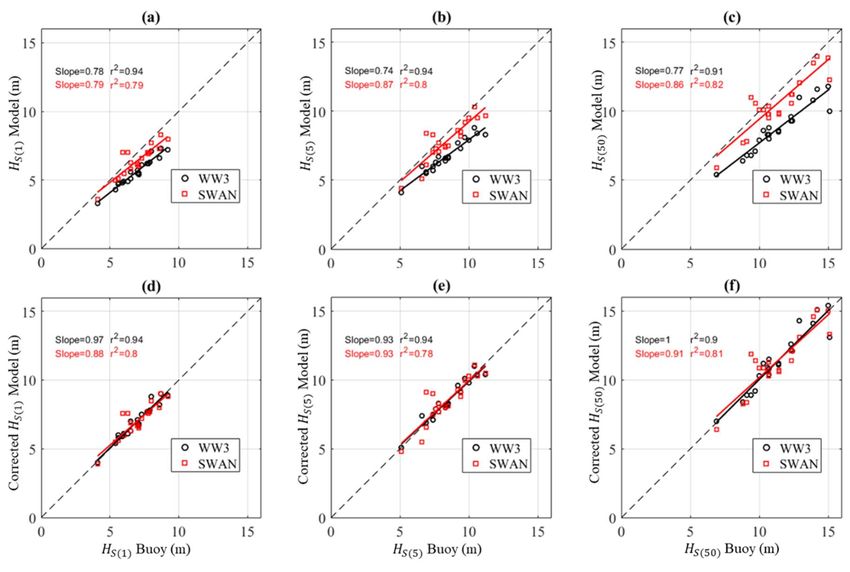
J. Mar. Sci. Eng. 2020, 8, 289                                                                          2 of 19

100-years) [4]. As specified by these international standards and guidelines, DLCs are to be constructed
for each design/environmental condition and different combinations of load types.
       Extreme wave statistics, like the 50-year significant wave height, Hs(50) , or 50-year sea states,
(Hs , Te )50 , are key metrics used to characterize extreme wave conditions for a host of ocean (offshore)
and coastal engineering applications [4], including offshore wind and marine energy. In marine energy,
the significant wave height recurring every fifty years on average, Hs(50) , has also been proposed as an
indicator of project risk using a relative risk ratio, Hs(50) /Hs(mean) [5,6]. In addition, the International
Electrotechnical Commission (IEC) recommends a design standard for wave energy converters (WEC)
that requires Hs(50) for building extreme condition DLCs for a WEC in a parked-survival condition,
and Hs(1) for building abnormal condition DLCs for a WEC in a parked condition with a fault
occurring [3]. Wave loads characterized by Hs(5) are required to build DLCs for tidal energy converters
in a parked-survival condition under an extreme hydrodynamic load occurring at a peak spring tide.
       Perhaps the most challenging analysis for the designer of a maritime structure is characterization
of the extreme n-year return period environmental conditions, which are then used to build design
load cases for evaluating the structural load responses. As the n-year return period events are often
well beyond the historic period of recorded data, the environmental conditions must be extrapolated
from the tails of extreme value distributions, which introduces uncertainty. Best practices, e.g., [1],
currently assume historic wave climates are stationary for the extreme value analysis techniques to
be valid and provide no methods for adjusting results, e.g., applying a scaling factor. According
to [7], the stationary assumption is reasonable for most applications. Trends reported for extreme
significant wave heights, particularly large n-year return period values, e.g., n = 100 years, are subject
to large statistical uncertainty [8]. Further, the uncertainties introduced by nonstationary trends are
likely less significant than those inherent in the extreme value analysis [9]. Nevertheless, research
on historical nonstationary regional trends in wave climates, including mean annual wave heights,
e.g., [10], extreme wave heights, e.g., [11], and inter-annual variability [12], suggests significant changes
in certain regions. Extreme values of significant wave height are increasing at a higher rate than mean
values [12,13]. While the observed trends reported in these studies vary, and there is currently no
consensus on the magnitude of these trends, consideration of their implications for design and project
risk assessment is warranted.
       International standards allow designers the flexibility to choose from a variety of statistical methods
to meet minimum design requirements, including simple univariate methods, e.g., peak-over-threshold
(POT) methods to calculate the design n-year wind, wave or current conditions, or relatively more
complex and rigorous bivariate methods, e.g., methods that calculate joint distributions (environmental
contours) of statistics characterizing environmental conditions, e.g., the inverse first-order reliability
method (IFORM) [14]. A recent review of univariate and bivariate statistical methods commonly used to
characterize extreme seas for ocean and coastal engineering applications is given by [7]. These extreme
wave statistical methods require the designer to find high-quality data sources of environmental
conditions with time series of sufficient duration based on guidance given by international standards,
e.g., [15], to accurately calculate return period conditions up to a hundred years or more. Time series
of bulk wave parameters like significant wave height, Hs , and energy period, Te , for example, can be
derived from in-situ measurements at a point or simulated model hindcast databases that provide full
coverage of the US coastline at resolutions up to 200 m, e.g., [16].
       Muir and El-Shaarawi [17] review data sources and their limitations for calculating n-year
significant wave height statistics: wave buoys are known to underestimate very large individual waves,
e.g., [18]; spatial coverage is limited beyond the point of observation; and measurement durations
are typically insufficient to calculate extreme sea state statistics [4]. Wave buoys, however, provide
reliable point observations of extreme significant wave height [18], and are the primary data source for
ground-truthing wave models.
       Spectral wave model hindcasts, using models like WAVEWATCH III®(WWIII) and Simulating
WAves Nearshore (SWAN), are an alternative data source for estimating extreme wave height statistics,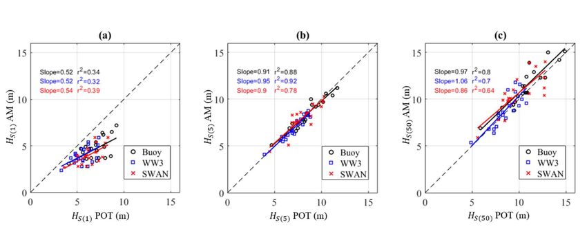
J. Mar. Sci. Eng. 2020, 8, 289                                                                       3 of 19

and are accepted for wave energy resource assessment and ocean engineering design when validated
with buoy measurements [1,2]. Model hindcasts also provide a means to address the noted limitations
of spatial coverage and measurement duration from buoy observations. Model performance studies
have demonstrated that the third-generation spectral wave models WWIII and SWAN can accurately
predict a host of wave energy resource statistics, and that their accuracy is significantly improved with
grid refinement [19,20]. Further, these models can examine the spatial variation of wave characteristics
at fine resolutions over larger regions encompassing different wave climates, e.g., [20,21]. These models,
however, underpredict large waves and extreme n-year significant wave heights. The main source of
this underbias is due to limitations of most wind reanalysis datasets, namely their inability to resolve
fine-scale high-energy wind gusts, e.g., [22,23]. Model performance studies commonly emphasize
predictions of common sea state statistics (bulk parameters) on average, e.g., Hs and peak period, Tp .
Several studies, however, have evaluated model performance predicting extreme significant wave
heights at return periods equal to or greater than 1-year, e.g., [7,19,24,25]; and some have examined
the use of simple linear correction methods to model-derived estimates of 100-year significant wave
heights, Hs(100) , to reduce model underbias relative to observation-derived estimates [24,25].
      Few studies have compared n-year return period significant wave heights, Hs(n) , derived using
different univariate extreme value analysis methods, e.g., [9], or compared Hs(n) derived using
univariate methods with the maximum n-year contour Hs values derived using bivariate methods,
e.g., [7]. Peak-over-threshold (POT) methods should be used with care and their results should be
checked with other methods, e.g., the annual maxima (AM) method, as a threshold value selection can
be subjective [1,9]. On the other hand, the AM method, the most common of the so-called block maxima
methods, can be subject to large uncertainty due to the small sample population [9]. In comparing
Hs(100) values estimated by univariate analysis (POT method) with maximum values of 100-year
environmental contours estimated using bivariate analysis, [7] found values agreed within one meter
for twelve of fifteen sites; but no systematic bias was observed.
      The present study investigates characterization of extreme wave conditions using different data
sources, buoy measurements vs. wave model outputs, and different methods allowed by design
standards, univariate methods (AM and POT) and the bivariate environmental contour method. The
goal is to understand how estimates of extreme wave characteristics are affected by both factors,
and to identify bias trends that may be adjusted. Compared to previous investigations, the present
study is much broader in scope in terms of the range of return periods evaluated, the different data
sources and methods used, and the number of wave sites and wave climates considered. We compare
model skill predicting extreme significant wave heights with 1, 5 and 50-year recurrence intervals,
Hs(1) , Hs(5) , and Hs(50) , at approximately two dozen buoy locations spanning several regional wave
climates along the US East and West Coasts. We also investigate the use of simple linear corrections to
model-derived extreme wave heights to improve their agreement with extreme wave heights derived
from buoy measurements. While this model performance evaluation does not consider spectral details
that can identify sources of model deficiencies, e.g., [26], it does provide an initial assessment of model
performance trends, including bias, and how performance may vary among different sites within a
regional wave climate and between different wave climates.

2. Methods

2.1. Study Region and Buoy Observations
     The study region, shown in Figure 1, encompasses potential wave energy project sites within the
economic exclusion zones (EEZ) along the US East and US West Coasts [27]. Only National Data Buoy
Center (NDBC) stations with hourly Hs and Te time series spanning long deployment periods of at
least 12.5 years were selected, to meet the ISO standard for estimating 50-year return period events
using the POT method, which recommends periods of record (POR) at a quarter of the desired return
period [15]. Missing data records in these time series reduced the POR to 12.21 years at Station 46050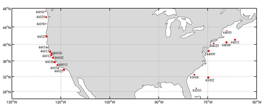
resolution of 200 m for coastal areas extending 20 km offshore and a resolution of 1–3 km for the
inner-shelf regions [21,29]. At thirty years or more, these model hindcasts exceed minimum
requirements for estimating extreme wave heights with return periods up to fifty years. and
time series outputs from these model hindcasts at three-hour intervals are used to estimate ( ) ,
and
( ) , Sci.
J. Mar. ( ) 8,and
Eng. 2020, 289 environmental contours ( , ) for comparison with those derived 4from of 19
measured (observation) ( , ) time series at NDBC stations at eight sites along the East Coast and
thirteen sites along the West Coast. For the initial comparison with observation-derived ( )
and to 10.62 years at Station 46054 (Figure 1, Table A1). Also, data in these time series were removed
estimates, the model-derived time series are limited to the observation POR at each station. These
to match modelled hindcast time series generated at three-hour intervals. Depths at these stations
POR-limited model-derived estimates are also used to determine the linear correction, to adjust raw
vary from 30 m (44009) to 4048 m (41002) p and are classified as intermediate and deep wave sites with
model-derived estimates to better match observation-derived values.
normalized peak frequencies of fP > 0.05 g/h.
Figure 1. NDBC stations along the US East Coast and the US West Coast selected for model performance
Figure 1. NDBC stations along the US East Coast and the US West Coast selected for model
study. The size of the circle indicates the period of record (POR) with the smallest indicating 11 years
performance
(46054), study.
and the The
largest size of 22
reflecting theyears
circle(e.g.,
indicates
44008).the period of record (POR) with the smallest
indicating 11 years (46054), and the largest reflecting 22 years (e.g., 44008).
2.2. Modelled Hindcast Data Sources
2.3. Univariate Extreme Value Analysis
The present study utilizes modelled hindcast data from several wave model studies to estimate
Thewave
extreme AM statistics:
method isa applied to estimate
WWIII 30-year model (v.5.08)( ) and hindcast
( ) from time series generated
study encompassing from
all US coastal
modelswith
waters anda buoy
spatialobservations
resolution offor comparison,
4 minutes (6–7 km) at three-hour intervals from
[28], a high-resolution all data
regional SWAN sources
32-year at
corresponding
model hindcastintervals
study for andthespanning
US Westthe samewith
Coast period of record
a spatial (POR) toofensure
resolution 200–300 consistency.
m [20], and This
a
method, which fits
high-resolution the yearly
regional SWAN maxima to a Gumbel
32-year model hindcast distribution,
study for theis an
USaccepted
East Coaststandard
with adetailed
spatial
in [1]. It isofsimple
resolution 200 mtoforimplement
coastal areasand extending
requires no 20 user inputs that
km offshore andcan introduce of
a resolution user
1–3bias
km like
for
peak-over-threshold
the inner-shelf regions (POT) methods.
[21,29]. It does,
At thirty years however, require
or more, thesea model
minimum POR ofexceed
hindcasts approximately
minimum 20
years [1]. While
requirements forthis requirement
estimating is not
extreme met heights
wave for ten sites, timeperiods
with return series for
upthese sites
to fifty strengthen
years. Hs andthe Te
correlation
time between
series outputs fromthethese
model- and
model measurement-derived
hindcasts at three-hour intervals( ) by
aredoubling the population
used to estimate Hs(1) , Hs(5of
),
samples
and Hs(50used
) and to derive the
environmental linear correction
contours ( H s , Tfor
e ) nmodel-derived
for comparison with
( ) estimates.
those As
derived the
fromsame POR
measured is
(observation) (Hs , Te ) time series at NDBC stations at eight sites along the East Coast and thirteen
sites along the West Coast. For the initial comparison with observation-derived Hs(n) estimates, the
model-derived Hs time series are limited to the observation POR at each station. These POR-limited
model-derived estimates are also used to determine the linear correction, to adjust raw model-derived
estimates to better match observation-derived values.
2.3. Univariate Extreme Value Analysis
The AM method is applied to estimate Hs(5) and Hs(50) from Hs time series generated from models
and buoy observations for comparison, at three-hour intervals from all data sources at corresponding
intervals and spanning the same period of record (POR) to ensure consistency. This method, which
fits the yearly maxima Hs to a Gumbel distribution, is an accepted standard detailed in [1]. It is
simple to implement and requires no user inputs that can introduce user bias like peak-over-threshold
(POT) methods. It does, however, require a minimum POR of approximately 20 years [1]. While this
requirement is not met for ten sites, Hs time series for these sites strengthen the correlation between the
model- and measurement-derived Hs(n) by doubling the population of samples used to derive the linear
correction for model-derived Hs(n) estimates. As the same POR is used for model and observation data
sources, the bias introduced by relaxing this requirement is consistent for both data sources. FollowingJ. Mar. Sci. Eng. 2020, 8, 289 5 of 19
comparisons of extreme wave height estimates between buoy observations and modelled data sources
that are limited to the buoy POR, estimates of extreme wave height using the entire 30 years of the
modelled hindcast data sources are also provided herein to examine the dependence of POR length;
especially for the buoy stations that did not meet the minimum POR requirements for the AM method.
For low return periods below 5 years, POT methods are recommended [4]. We apply a POT
method to estimate Hs(1) utilizing the generalized Pareto distribution model (GPD), which has been
broadly applied for estimating extreme wave heights, e.g., [7,24,30,31]. For a Type I GPD model, the
shape parameter is zero [30], and the cumulative distribution function is
x − µ
F(x) = 1 − exp − (1)
σ
where x is the extreme significant wave height associated with an individual storm, µ is the threshold
significant wave height used to filter the sample population of significant wave heights in the time
series, and σ, the scaling parameter, is the mean value of the excess (x − µ).
As with other studies, the threshold is selected to be low enough to maintain a minimum
population of samples to ensure a robust model fit that limits variance, while high enough to be
characterized as a tail sample by the GPD model. Quantile–quantile plots are used to identify the
threshold that provides the best-modelled distribution fit [30]. The Wald–Wolfowitz Runs (WWR) test
is used to check that samples are independent [32]. The most notable disadvantage of POT method is its
sensitivity to the threshold value selected. Despite best efforts to objectively select threshold values, it
is difficult not to introduce user bias. Threshold values selected in the present study were 99-percentile
Hs values on average, with a standard deviation of several tenths of a meter. For comparison, [7]
found that 98-percentile values provided the best regional model fits along the Canadian Pacific Coast
when using a Type II GPD model. Vanem [9], in comparing estimates of Hs(100) and Hs(20) using block
maxima and POT methods at a wave site in the North Atlantic, selected 99.5 and 99.95-percentile values
for his study to examine the sensitivity of extreme significant wave height to the threshold value.
2.4. Linear Correction of Modelled Extreme Wave Heights
A simple linear correction method proposed by Stephens and Gorman [25] is applied to improve
the agreement between Hs(n) values derived from modelled and measured (observation) data sources
at the observation-limited POR, where modelled Hs(n) values are scaled by the average relative bias
among the study sites,
1 XN Mod. Hs(n), i − Obs. Hs(n),i
s = (2)
N i=1 Mod. Hs(n), i
where N is the number of sites, and i is the site index. This correction scaling constant, s, should not be
confused with the average mean bias, B, which considers bias relative to the measurement-derived
value to evaluate the model performance.
To compare the goodness of fit between the model and measurement-derived Hs(n) values, a
linear regression best-fit line is plotted along with the line of equivalence, and r2 , and slope (m) values
are reported (Figures 2–4). The mean absolute relative bias (B) is calculated as a summary statistic to
quantify this comparison,
1 XN Mod. Hs(n), i − Obs. Hs(n),i
B = (3)
N i=1 Obs. Hs(n), i
Here, the bias is relative to the measured data source (observation) rather than the modelled data
source as calculated for the scaling factor using (2).J. Mar. Sci. Eng. 2020, 8, 289 6 of 19
2.5. Bivariate Extreme Value Analysis (Environmental Contours)
Environmental contours for 1-, 5- and 50-year sea states within the (Hs , Te ) parameter space are
created using an inverse first-order reliability method (IFORM) with principal components analysis
(PCA) and inverse Gaussian and normal distribution models as described in [14]. This method is
similar to the traditional IFORM summarized in [1]. PCA is applied prior to the IFORM to generate an
uncorrelated representation of (Hs , Te ) in terms of principal components (C1 , C2 ) that result in better
fitting contours. The probability density function of the principal component C1 is parameterized with
an inverse Gaussian (Wald) distribution model
λ(x − µ)2
r
λ
f (x) = exp−
(4)
2πx3 2µ2 x
with parameters µ and λ determined by maximum likelihood estimation (MLE). Values of C2 are
binned based on their corresponding C1 values. Probability density functions of C2 conditioned on C1
are parameterized with a normal (Gaussian) distribution model
1 x−µ 2
" #
1
f (x) = √ exp − (5)
σ 2π 2 σ
with estimates of the C2 normal distribution parameters µ and σ as a function of C1 for each bin
modelled with the fitting functions
fµ (C1 ) = β0 + β1 C1 (6)
fσ (C1 ) = γ0 + γ1 C1 + γ2 C21 (7)
with linear coefficients β0 , β1 , and quadratic coefficients γ0 , γ1 , γ2 , determined by a least square
regression procedure. The fitted inverse Gaussian distribution model for C1 and fitted normal
distributions models for C2 , as a function of the mean value of C1 for each bin are used to construct
an environmental contour in principal component space for a given return period using the IFORM,
which is then transformed back to the (Hs , Te ) parameter space using the equations
C1i v1,1 + C2i − s v1,2
Hsi = (8)
v21,1 + v21,2
C1i v1,2 + C2i − s v1,1
Tei = (9)
v21,1 + v21,2
where v1,1 , v1,2 , v2,1 , and v2,2 are the PCA rotation coefficients and s is the required adjustment applied
to the principal component, C2i , to ensure it is greater than zero in the principal components space.
When negative values of Hsi occur at very low values, an artifact of the PCA not being constrained
by limitations of the wave physics, they are set to zero. As these sea state occurrences delineate very
low wave heights at the base of the contour line, they are not significant for characterizing extreme
wave loads.
3. Results
3.1. Comparison of Univariate Methods
Estimates of Hs(n) derived using both AM and POT methods are compared at all study buoy
stations, and for all three data sources, in scatter plots shown in Figure 2. Again, for this comparison, the
periods of record of model-derived data sources were reduced to match those of the observation-derived
data sources for each buoy station—not the entire 30-year POR. The perfect agreement line and slopeJ. Mar. Sci. Eng. 2020, 8, 289 7 of 19
and r2 values of linear regression fits are shown to quantify how well estimates are correlated using
AM and POT methods applied to the same data source.
The comparison of Hs(1) estimates derived using the AM and POT methods, Figure 2a, is presented
to illustrate the problem that arises when using the AM method for low return period events, and
why it is not recommended practice [4]. The present study adopts the POT method for estimating
HJ. Mar.inSci.subsequent
Eng. 2020, 8, 3analyses.
FOR PEER REVIEW
Hs(1) estimates derived using the AM method are significantly lower 7 of 19
s(1)
than those derived using the POT method, with all points falling below the line of equivalence. As
( ) magnitude.
indicated
Low values indicate large scatter for all data sources, i.e., large and frequent
by the low values for regression slope, this underbias increases with the Hs(1) magnitude.
discrepancies
Low betweenlarge
r2 values indicate estimates
scatterwhen
for allusing these two
data sources, i.e.,different
large andmethods.
frequentBy comparison,
discrepancies Figure
between
2b,c shows that
estimates when using and
( ) these two estimates are in much better agreement. Points
( )different methods. By comparison, Figure 2b,c shows that H are nearly equally
s(5) and
distributed about the line of equivalence, slopes are close to 1 and high
Hs(50) estimates are in much better agreement. Points are nearly equally distributed about the line of values show significant
correlations slopes
equivalence, between are results
close tousing theser2two
1 and high different
values methods applied
show significant to the
correlations same results
between data source.
using
Agreement is relatively better
these two different methods applied to for estimates, but the good agreement for both
( )the same data source. Agreement is relatively better ( ) , and
for Hs((5))
support using the AM
goodmethod for the
forpresent
both Hstudy due to its simpler implementation. Nevertheless,
estimates, but the agreement s(5) , and Hs(50) support using the AM method for the
while discrepancies between estimates using
present study due to its simpler implementation. Nevertheless, the AM and POT method
while are random,
discrepancies theyestimates
between can vary
significantly,
using the AM similar
and POT tomethod
[9]. Thearemagnitude
random, and theyfrequency of these large
can vary significantly, discrepancies
similar to [9]. Theincrease
magnitudewith
return period, but are less sensitive to the POR or data source.
and frequency of these large discrepancies increase with return period, but are less In some cases, estimates
( ) sensitive to theare in
perfect
POR or agreement,
data source.while, In somein other cases,
cases, ( ) estimates
Hs(50) estimates are indiffer by agreement,
perfect more than 2while,
m. in other cases,
Hs(50) estimates differ by more than 2 m.
Figure 2. Scatter diagrams comparing Hs(n) estimates at all buoy stations using the annual maxima
Figureand
(AM) 2. Scatter diagrams comparing
peak-over-threshold ( ) estimates
(POT) methods appliedattoall
thebuoy
samestations using(buoy
data source the annual maxima
observations,
(AM) and peak-over-threshold (POT) methods applied to(a)
theHsame data source (buoy observations,
WWIII hindcast predictions, SWAN hindcast predictions): s(1) ; (b) Hs(5) ; (c) Hs(50) . Note that, for
WWIII hindcast predictions, SWAN hindcast predictions): (a)
these comparisons, the periods of record of model-derived data sources ( ) ; (b) ) ; (c)
were( reduced ) . Notethose
( match
to that,
for these comparisons, the periods of record of model-derived data sources
of the observation-derived data sources for each buoy station given in Tables A1–A3. were reduced to match
those of the observation-derived data sources for each buoy station given in Tables A1, A2 and A3.
3.2. Comparison of Data Sources for Univariate Analysis
3.2. Comparison of Data Sources for Univariate Analysis
Comparisons between model- and observation-derived Hs(1) values (POT Method), and Hs(5)
and H Comparisons
s(50) values (AMbetween model-
Method) areand observation-derived
visualized values 3a–c
in scatter plots (in) Figure (POTand Method), and in
summarized ( )
and A1–A3.
Tables ( ) values (AM
These Method)
tables summarizeare visualized
the raw in
and scatter plots
corrected H in
s(n) Figure
derived 3a–c
by and
model summarized
hindcasts in
for
Tables A1, A2 and A3. These tables summarize the raw and corrected
each site with the percent relative bias in parentheses. Again, for this comparison, ( ) derived by model
the periods of record
hindcasts
of for eachdata
model-derived site sources
with thewerepercent relative
reduced bias inthose
to match parentheses. Again, for this comparison,
of the observation-derived the
data sources
periods of record of model-derived data sources were reduced
for each buoy station—not the entire 30-year POR. Model-derived H s(1) , H s(5to
) , match
and H s(50)those of the
values based
observation-derived
on data sources
the full “30-year” record for each buoy
of the modelled station—not
hindcasts, 30 yearsthe
for entire
WWIII30-year
and 32 POR.years Model-derived
for SWAN, are
( ), ( ) , and ( ) values based on the full “30-year” record of the modelled hindcasts, 30 years
provided in Tables A1–A3 to examine the sensitivity of the model-derived estimates to POR.
for WWIII and 32 years for H
With the exception of SWAN, are provided
s(n) , derived from SWANin Tables A1, A2 at
hindcasts and A3 to examine
Stations 46026 and the46054,
sensitivity
and
Hofs(the
50) , model-derived
derived from SWAN estimates to POR.at Station 41004, the raw values of Hs(n) derived using both
hindcasts
models, With the exception of ( ) , derived
at the observation limited POR, are from SWAN
lower thanhindcasts at Stations
those derived from buoy46026observations,
and 46054, and as
shown, derived
in Figurefrom
3a–cSWAN hindcasts at Station 41004, the raw values of
and Tables A1–A3. This underbias for model-derived H sderived
(n) is using both
not sensitive
( ) ( )
models, at the observation limited POR, are lower than those derived from buoy observations, as
shown in Figure 3a–c and Tables A1, A2 and A3. This underbias for model-derived ( ) is not
sensitive to return period based on the slopes of the linear regression fits. For WWIII, the regression
slope m = 0.78 for model-derived ( ) , 0.74 for ( ) , and 0.77 for ( ) . For SWAN, the regression
slope m = 0.79 for model-derived , 0.87 for , and 0.86 for . Model performanceJ. Mar. Sci. Eng. 2020, 8, 289 8 of 19
to return period based on the slopes of the linear regression fits. For WWIII, the regression slope
m = 0.78 for model-derived Hs(1) , 0.74 for Hs(5) , and 0.77 for Hs(50) . For SWAN, the regression slope
m = 0.79 for model-derived Hs(1) , 0.87 for Hs(5) , and 0.86 for Hs(50) . Model performance predicting
extreme wave heights over a broad range of return periods is clearly improved by increasing model
spatial resolution. The average model relative absolute bias for WWIII-derived Hs(1) , Hs(5) , and
Hs(50) estimates is approximately 20%, compared to approximately 10% for those derived by the
SWAN model.
Raw model- and observation-derived estimates are generally well-correlated based on r2 values,
and these correlations are insensitive to return period. Correlations of linear regression fits, shown in
Figures 3, 4 and 5a,c, did not improve by separating the study sites by regional wave climate (East Coast
and West Coast). Correlations are significantly better between raw WWIII model-derived estimates
(r2 ≥ 0.91) and observation-derived estimates than those for the raw SWAN model-derived estimates
(r2 ≥ 0.79), likely due to the aforementioned SWAN model-derived outliers at Stations 41004, 46026
and 46054.
Linear regressions (not shown) indicate significantly stronger correlations and agreement between
model and observation-derived 98-percentile significant wave height estimates, Hs(98%) , compared to
Hs(1) , Hs(5) , and Hs(50) : m = 0.93, with r2 = 0.97 for WWIII model-derived 98-percentile wave heights,
Hs(98%) ; and m = 0.98 for SWAN model-derived Hs(98%) . In other words, the models perform quite
well, predicting extreme wave heights up to 98-percentile values. It is the extreme wave heights at
return periods n ≥ 1-year for which model underbias is significant. Hs(1) are about twice the height of
Hs(98%) .
As shown in Tables A1–A3, raw model-derived Hs(n) estimates using full 30-year POR are
generally within 10% of values using the lower buoy station limited POR. However, discrepancies are
particularly large, equal to or exceeding 10%, for several stations. These large discrepancies are not
generally associated with low periods of record. Raw model-derived Hs(1) estimates using the POT
method, as expected, are least sensitive to the POR length. Discrepancies are all below 10% with the
exception of SWAN model-derived Hs(1) estimates at Stations 46026 and 46054. As the return period
increases and the AM method is employed, the number of large discrepancies increases. More large
discrepancies are observed for SWAN model-derived estimates than WWIII.
3.3. Linear Correction of Modelled Extreme Wave Heights
Corrections applied to the model-derived Hs(n) , with the scaling factors calculated using
Equation (2), significantly improve the agreement between model and observation-derived values. The
average relative absolute bias for WWIII is reduced to 3%–4%, and that for SWAN to 6%–7%. Comparing
scatter plots with raw model-derived estimates, Figure 3a–c, to corrected model estimates, Figure 3d,e,
illustrates how this simple correction adjusts values to better align with lines of equivalence. Increases
in the slopes (m) of the linear regression fits quantify these improvements, increasing m = 0.74–0.78 to
0.90–0.97 for WWIII model-derived estimates, and increasing m = 0.79–0.82 to 0.88–0.93 for the SWAN
model-derived estimates. As expected, discrepancies between model-derived Hs(n) estimates using
full 30-year POR and those based on the lower limited POR of the buoy station are similar, whether
comparing raw or corrected values.J. Mar. Sci. Eng. 2020, 8, 289 9 of 19
J. Mar. Sci. Eng. 2020, 8, 3 FOR PEER REVIEW 9 of 19
Figure 3.
Figure 3. Scatter
Scatterplots at at
plots twenty-one
twenty-one NDBC NDBC stations comparing
stations comparing( )H , s(1)(, )H , and
s(5) , and( ) derived
Hs(50) derived from
from
models with those derived from in-situ observations at NDBC stations. Black circles indicate aa
models with those derived from in-situ observations at NDBC stations. Black circles indicate
comparison
comparison of of WWIII
WWIII model-derived
model-derived values values with
with observation-derived
observation-derived values. values. Red Red squares
squares indicate
indicate aa
comparison
comparison of SWAN model-derived values with observation-derived values. Dashed lines represent
of SWAN model-derived values with observation-derived values. Dashed lines represent
lines
lines of
of equivalence.
equivalence. Solid Solid lines
lines represent
represent lines
lines of
of best fit from
best fit from linear
linear regression:
regression: (a), raw Hs(1) models
(a), raw
( ) models
vs Hs((1)) buoy
vs. buoy (POT (POT method);
method);(b), (b),raw Hs(5) models
raw ( ) modelsvs. H vss ( 5 ) buoybuoy
( )
(AM(AM method); (c), raw
method); (c),Hsraw
(50)
vs. Hs(vs
modelsmodels 50 ) buoy buoy
(AM method); (d), corrected H models vs.
(AM method); (d), corrected ( ) models vs ( ) buoy (POT method);
s ( 1 ) H s ( 1 ) buoy (POT method); (e),
( ) ( )
corrected H models vs. H buoy (AM method); (f), corrected
(e), corrected ( ) models vs ( ) buoy (AM method); (f), corrected ( ) models vs ( ) buoy
s ( 5 ) s ( 5 ) H s ( 50 ) models vs. H s ( 50 ) buoy (AM
method). Note that raw estimates (a–c) are adjusted by linear correction with scaling factor, s, using
(AM method). Note that raw estimates (a,b,c) are adjusted by linear correction with scaling factor, s,
(1) to generate corrected estimates (d–f). Note that, for these comparisons, the periods of record of
using (1) to generate corrected estimates (d,e,f). Note that, for these comparisons, the periods of record
model-derived data sources were reduced to match those of the observation-derived data sources for
of model-derived data sources were reduced to match those of the observation-derived data sources
each buoy station given in Tables A1–A3.
for each buoy station given in Tables A1, A2 and A3.
3.4. Environmental Contours
3.4. Environmental Contours
Environmental contours delineating the 1-year, 5-year and 50-year extreme sea states are shown
Environmental
for five selected buoycontours
stations delineating
along the EasttheCoast,
1-year,Figure
5-year4,and
and50-year extreme
five selected sea states
stations along are
theshown
West
for five selected buoy stations along the East Coast, Figure 4, and five selected stations
Coast, Figure 5. These stations were selected to highlight the effect of latitude on extreme sea states foralong the West
Coast,two
these Figure 5. These
US wave stations
climate wereEach
regions. selected to highlight
plot compares the effect
contours of latitude
generated onthree
using extreme sea states
different data
for these two US wave climate regions. Each plot compares contours generated
sources: buoy observations, WWIII hindcast data, and SWAN hindcast data. For all stations, using three different
these
data sources: show
comparisons buoy that
observations, WWIII hindcast
the model-derived contours data, and expected
capture SWAN hindcast data.
trends that For the
affect all stations,
contour
size as measured by the range of Hs(n) and Te(n) . As expected, the maximum values of Hs(n)affect
these comparisons show that the model-derived contours capture expected trends that the
increase
contour size as measured by the range of
with return period and with latitude along both( coasts, ) and .
as (more
) As expected, the maximum values
energetic wave climates are found in of
( ) increase
northern with[21,29].
latitudes return period
There isand
nowith latitude
similar along both
north–south trend coasts, as more energetic
in maximum values ofwave
Te(n) .climates
are found in northern latitudes [21,29]. There is no similar north–south trend
WWIII model-derived contours are generally smaller than those based on buoy observations, in maximum valuesbut
of
).
the( WWIII model-based 5-year and 50-year contours at East Coast Station 44025 are nearly identical to
thoseWWIII
derivedmodel-derived contours
from observations. are West
For the generally
Coast,smaller
WWIIIthan those based
and SWAN on buoy observations,
model-derived contours are
but the but
similar, WWIII model-based the
both underpredict 5-year
Hs(n)and
and50-year contours
Te(n) range compared at East
to theCoast Station
contour based44025 are nearly
on observations.
identical to those derived from observations. For the West Coast, WWIII and
For the East Coast, SWAN model-derived contours are generally in good agreement. Similar SWAN model-derived
contours
to are similar, are
[7], discrepancies butsmall
both underpredict the of( periods
over a wide range ) and (and) range
wavecompared
heights for toEast
the contour based
Coast Station
on observations.J. Mar. Sci. Eng. 2020, 8, 3 FOR PEER REVIEW 10 of 19
ForSci.
J. Mar. theEng.
East Coast,
2020, SWAN model-derived contours are generally in good agreement. Similar
8, 289 10 of 19 to
[7], discrepancies are small over a wide range of periods and wave heights for East Coast Station
44005 for 1-year and 5-year contours, and 41004 and 41010 for all n-year contours. At the East Coast
44005 for 1-year and 5-year contours, and 41004 and 41010 for all n-year contours. At the East Coast
stations, SWAN
stations, SWAN model-derived
model-derivedcontours
contoursexhibit
exhibitaalonger rangethan
longer Te((n)) range thanWWIII
WWIIIcontours,
contours, and
and areare
in in
good
goodagreement
agreement with
withbuoy
buoycontours,
contours,e.g.,
e.g., Stations
Stations 44005, 41004,and
44005, 41004, and41010
41010for
for1-year
1-yearand
and 5-year
5-year
contours. However, at a few stations, the SWAN contours overestimate the
contours. However, at a few stations, the SWAN contours overestimate the Te(n() range, ) range, e.g., 50-year
e.g., 50-year
contours
contoursat at
Stations
Stations44005
44005and
and44025.
44025.
Figure
Figure 4. 4. Comparisonofofenvironmental
Comparison environmentalcontours
contours atat five
five selected
selected East
EastCoast
Coastbuoy
buoystations
stationsbased
based onon
three different data sources: buoy observations (solid line), WWIII (dotted line) and SWAN (dashed
three different data sources: buoy observations (solid line), WWIII (dotted line) and SWAN (dashed
line). Each row shows contours at a given buoy station at latitudes in descending order from north to
line). Each row shows contours at a given buoy station at latitudes in descending order from north to
south, and 1-, 5- and 50-year contours shown from left to right: (a) 44005, 1-year; (b) 44005, 5-year; (c)
south, and 1-, 5- and 50-year contours shown from left to right: (a) 44005, 1-year; (b) 44005, 5-year; (c)
44005, 50-year; (d) 44025, 1-year; (e) 44025, 5-year; (f) 44025, 50-year; (g) 44009, 1-year; (h) 44009, 5-year;
44005, 50-year; (d) 44025, 1-year; (e) 44025, 5-year; (f) 44025, 50-year; (g) 44009, 1-year; (h) 44009,
(i) 44009, 50-year; (j) 41004, 1-year; (k) 41004, 5-year; (l) 41004, 50-year; (m) 41010, 1-year; (n) 41010,
5-year; (i)(o)
5-year; 44009, 50-year;
41010, 50-year.(j) 41004, 1-year; (k) 41004, 5-year; (l) 41004, 50-year; (m) 41010, 1-year; (n)
41010, 5-year; (o) 41010, 50-year.J. Mar. Sci. Eng. 2020, 8, 289 11 of 19
J. Mar. Sci. Eng. 2020, 8, 3 FOR PEER REVIEW 11 of 19
Figure 5. Comparison of environmental contours at five selected West Coast buoy stations based on
Figure 5. Comparison of environmental contours at five selected West Coast buoy stations based on
three different data sources: buoy observations (solid line), WWIII (dotted line), and SWAN (dashed
three different data sources: buoy observations (solid line), WWIII (dotted line), and SWAN (dashed
line). Each row shows contours at a given buoy station at latitudes in descending order from north to
line). Each row shows contours at a given buoy station at latitudes in descending order from north to
south, and 1-, 5- and 50-year contours shown from left to right: (a) 46029, 1-year; (b) 46029, 5-year; (c)
south, and 1-, 5- and 50-year contours shown from left to right: (a) 46029, 1-year; (b) 46029, 5-year; (c)
46029, 50-year; (d) 46027, 1-year; (e) 46027, 5-year; (f) 46027, 50-year; (g) 46013, 1-year; (h) 46013, 5-year;
46029, 50-year; (d) 46027, 1-year; (e) 46027, 5-year; (f) 46027, 50-year; (g) 46013, 1-year; (h) 46013,
(i) 46013, 50-year; (j) 46042, 1-year; (k) 46042, 5-year; (l) 46042, 50-year; (m) 46011, 1-year; (n) 46011,
5-year;
5-year;(i)(o)
46013,
46011,50-year;
50-year.(j) 46042, 1-year; (k) 46042, 5-year; (l) 46042, 50-year; (m) 46011, 1-year; (n)
46011, 5-year; (o) 46011, 50-year.
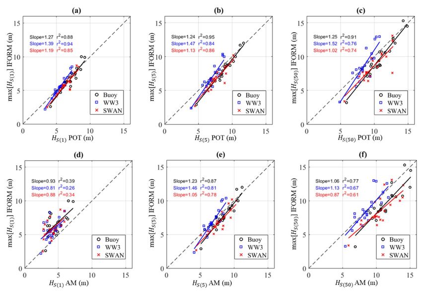
Maximum values of Hs(n) on each contour are compared with values derived using POT and
AMMaximum
methods invalues
Figureof6 for(the
) on eachdifferent
three contourdataaresources
compared with values
evaluated. Again,derived usingthe
results using POTAM and
AM methods
method in Figure
are shown 6 for thedifferences
to highlight three different
at thisdata
lowsources evaluated.
return period Again,
and why this results
methodusing
should the AM
not
method are shown to highlight differences at this low return period and why this method should
be used for low return period estimates. As shown in Figure 6a–c, the maximum values of H s(n) onnot
beeach
usedcontour
for lowagree
return period
well withestimates.
Hs(n) valuesAsestimated
shown in using
Figurethe
6a,b,c,
POT the maximum
method, values
similar to [7].ofValues
( ) on
estimated using the AM method agree less well, likely because the univariate POT
each contour agree well with ( ) values estimated using the POT method, similar to [7]. Valuesmethods are more
consistent with those used in environmental contour methods; this disagreement is more pronounced
estimated using the AM method agree less well, likely because the univariate POT methods are more
for 50-year estimates compared to 5-year, and shows sensitivity to data source at this higher return
consistent with those used in environmental contour methods; this disagreement is more pronounced
period. Maximum Hs values on 5-year and 50-year contours exhibit a systematic underbias compared
for 50-year estimates compared to 5-year, and shows sensitivity to data source at this higher return
period. Maximum values on 5-year and 50-year contours exhibit a systematic underbias
compared to estimates of ( ) and ( ) based on univariate methods, when using observation
and SWAN model hindcast datasources.J. Mar. Sci. Eng. 2020, 8, 289 12 of 19
to estimates of Hs(5) and Hs(50) based on univariate methods, when using observation and SWAN
J. Mar. Sci. Eng. 2020, 8, 3 FOR PEER REVIEW 12 of 19
model hindcast datasources.
Figure
Figure 6. 6. Comparison
Comparison ofof the
the maximum
maximum values
values of of Hs on on each
each contour
contour with
with values
values derived
derived using
using
univariate methods for all buoy stations. Peak-over-threshold (POT) method: (a) s((1)); (b) s((5));; (c)
univariate methods for all buoy stations. Peak-over-threshold (POT) method: (a) H ; (b) H (c)
Hs((50)).. Annual
Annualmaxima
maxima (AM)
(AM) method:
method: (d)
(d) Hs((1));; (e)
(e) Hs((5));; (f)
(f) Hs((50))..
4. Discussion
4. Discussion
The present study demonstrates that extreme significant wave height estimates using the AM
The present study demonstrates that extreme significant wave height estimates using the AM
method and POT method can vary significantly, but estimates using the simpler AM method at higher
method and POT method can vary significantly, but estimates using the simpler AM method at
return periods starting at n = 5-years are generally in good agreement with the POT method, even
higher return periods starting at n = 5-years are generally in good agreement with the POT method,
when the minimum 20-year POR requirement is not met [1]. The AM method should, therefore, be
even when the minimum 20-year POR requirement is not met [1]. The AM method should, therefore,
considered for estimating higher return period events to avoid the inherent user bias problems of the
be considered for estimating higher return period events to avoid the inherent user bias problems of
POT method. The POT method should always be used for low return period events, e.g., n = 1-year [4].
the POT method. The POT method should always be used for low return period events, e.g., n =
For estimating n-year significant wave heights between one and five years, the results of both methods
1-year [4]. For estimating n-year significant wave heights between one and five years, the results of
should be compared with a preference for the POT method and good engineering judgment and
both methods should be compared with a preference for the POT method and good engineering
understanding of the risks of overdesign and underdesign.
judgment and understanding of the risks of overdesign and underdesign.
Raw model-derived estimates of extreme significant wave height with return periods equal to or
Raw model-derived estimates of extreme significant wave height with return periods equal to
greater than 1 year exhibit a systematic underbias compared to observation-derived estimates. This
or greater than 1 year exhibit a systematic underbias compared to observation-derived estimates. This
finding, along with similar observations made in previous studies for H [24,25], indicates that raw
finding, along with similar observations made in previous studies fors(100() ) [24,25], indicates that
model-derived estimates should not be used to characterize extreme wave or sea state conditions with
raw model-derived estimates should not be used to characterize extreme wave or sea state conditions
return periods equal to or greater than 1 year for WEC design or project risk assessment. While raw
with return periods equal to or greater than 1 year for WEC design or project risk assessment. While
model-derived estimates are still valuable for the relative comparison of project risks between sites, or
raw model-derived estimates are still valuable for the relative comparison of project risks between
the spatial distribution of extreme wave conditions, they should be corrected when used to build DLCs
sites, or the spatial distribution of extreme wave conditions, they should be corrected when used to
for WEC design.
build DLCs for WEC design.
Applications of grid refinement and improved model physics and atmospheric forcing data can
Applications of grid refinement and improved model physics and atmospheric forcing data can
significantly reduce model bias in predicting extreme wave heights, including those with high return
significantly reduce model bias in predicting extreme wave heights, including those with high return
periods up to 50 years. However, simple linear correction methods applied to model-derived estimates,
periods up to 50 years. However, simple linear correction methods applied to model-derived
estimates, ( ) , as demonstrated herein and in other studies [24,25], may offer a more economical
approach to offset their observed underbias relative to observation-derived estimates. Without
correction, design load cases for extreme sea states based on ( ), ( ) , and ( ) could beJ. Mar. Sci. Eng. 2020, 8, 289 13 of 19
Hs(n) , as demonstrated herein and in other studies [24,25], may offer a more economical approach
to offset their observed underbias relative to observation-derived estimates. Without correction,
design load cases for extreme sea states based on Hs(1) , Hs(5) , and Hs(50) could be significantly
underestimated [3], and likewise for wave energy project risks based on Hs(50) and Hs(50) /Hs(mean) [6].
Model-derived environmental contours predict similar trends to those derived by buoy
observations, but the frequency and magnitude of discrepancies between model- and
observation-derived contours is mixed, similar to [7]. In some cases, model-derived contours are in
excellent agreement with buoy-derived contours, but generally they underestimate the Hs and Te range,
similar to model-derived estimates using univariate methods. In contrast to [7], results herein indicate a
tendency for maximum Hs values on contours to exhibit a systematic underbias compared to estimates
based on univariate methods. Unlike univariate methods, there is no discernible improvement in the
agreement of model-derived contours with observation-derived contours by increasing model spatial
resolution. Further, simple linear correction methods cannot be applied to improve this agreement.
To summarize the main findings of the present study and their implications for design and project
risk assessment, consider extreme wave height characterization based on Hs(50) for NDBC Stations
46029 amd 46050. The various estimates of Hs(50) are given in Table A3. Buoy observations at Station
46029 are limited to only fourteen years at this site, below the 20-year minimum requirement for
estimating a 50-year return period event using the AM method [1], but above the 12.5-year minimum
requirement for estimating this event using the POT method [15]. The observation-derived estimate of
Hs(50) = 14.3 m using the POT method described herein, therefore, follows the best-practice standard.
Using the AM method, which does not follow best practice, Hs(50) = 14.2 m. Finally, the maximum
value of Hs on the 50-year contour generated by bivariate analysis is 15.3 m. In this case, one would
typically select Hs(50) = 15.3 m to characterize the extreme wave condition for WEC design and project
risk assessment. It follows best practice and it is a significantly larger and more conservative value
than values given using the univariate methods.
For comparison, at Station 46050, with a POR of twelve years, Hs(50) = 14.9 m using the POT
method and Hs(50) = 15.1 m using the AM method. The maximum value of Hs on the 50-year contour
is 14.5 m. In this case, the minimum requirement for the POT method is closely met, and Hs(50) = 14.9
m would be justified; however, one could also make a case for choosing the more conservative value
Hs(50) = 15.1 m based on the AM method, even though the buoy POR does not satisfy the 20-year
minimum requirement. Corrected model-derived estimates base on the full 30-year records, which do
satisfy standard requirements for using the AM method, could also be evaluated. For Station 46029,
Hs(50) = 13.8 m, using model-corrected WWIII hindcast data, and Hs(50) = 14.7 m, using model-corrected
SWAN hindcast data. With these results, the largest and most conservative SWAN model-derived
estimate Hs(50) = 14.7 m would be justified if the reduced risk of failure is worth the added cost. For
Station 46050, Hs(50) = 14.2 m using the AM method based on the 30-year model-corrected SWAN
hindcast data. As this is less than the observation-derived Hs(50) = 14.9 m using the POT method, one
would typically choose the larger, more conservative value; however, both values satisfy standard
practice requirements, and one could alternatively choose the lower value if the added structural
design cost is deemed not worth the reduced risk of failure.
5. Conclusions
The results presented herein demonstrate several challenges in estimating n-year return period
extreme significant wave height, Hs(n) , or sea state, (Hs , Te )n , to characterize extreme wave conditions
for WEC design and project risk assessment. Periods of record for observation-derived estimates
typically do not meet the minimum requirement to estimate 50-year return period events, i.e., twelve
and a half years for the POT method [15], or twenty years for the AM method [1]. When different
methods, e.g., POT and AM, can be used, discrepancies between them are random and can exceed 20%.
While validated model hindcasts extend the POR and spatial coverage of data sources, model-derived
estimates are systematically underbiased compared to those derived from buoy observations.J. Mar. Sci. Eng. 2020, 8, 289 14 of 19
Within the scope of the present study, which limits its investigation to coastal waters along the
US East and West Coasts, buoy observations that are less than approximately two decades, model
hindcast data limited to three decades, and the assumption of stationary wave climate trends inherent
in most extreme value analyses, results support the use of simple linear corrections to model-derived
estimates, Hs(n) , as a practical way to extend the POR and spatial coverage of extreme wave statistics,
while correcting for underbiased discrepancies compared to observation-derived estimates.
Additional efforts are needed to more rigorously verify these correction methods using a
split-sample method, with a population of sea state statistics derived from one set of observations to train
the correction scaling, and a population of sea state statistics derived from another set of observations
to validate it. Although model underbias is not observed to be affected by differences in regional
wave climates, regional effects on scaling factors should not be ruled out and, therefore, should be
investigated further. While these simple linear correction methods cannot improve agreement between
model- and observation-derived environmental contours, other correction or training techniques,
e.g., machine learning, should be investigated to realize similar benefits for bivariate extreme sea
state analysis.
Characterization of extreme wave conditions for WEC design and project risk assessment is
improved by comparing estimates using different methods and data sources. In this comparison,
standard best practices should be followed to the extent possible, but engineering judgment that
balances risk of failure and cost must be exercised.
Although the effect of nonstationary wave climate trends on extreme wave conditions is not the
focus of the present investigation, it may have significant implications for WEC design and project risk
assessment. Simple linear adjustments to extreme wave height estimates, Hs(n) , based on reported
estimates of their projected increases could be applied, but further research is needed to reach consensus
on the magnitude and regional distribution of nonstationary trends in extreme wave height.
Author Contributions: Conceptualization, V.S.N.; methodology, V.S.N., B.E.S. and S.A.; software, S.A. and B.E.S.;
wave model validation, V.S.N., M.N.A., T.W., Z.Y. and R.H.; formal analysis, V.S.N., S.A. and B.E.S.; Investigation,
V.S.N. and S.A.; resources, V.S.N. and S.A.; modelled data curation, S.A., T.W. and M.N.A.; writing—original
draft preparation, V.S.N.; writing—V.S.N., S.A. and B.E.S.; figures and tables, V.S.N., S.A. and B.E.S.; supervision,
V.S.N.; project administration, V.S.N.; funding acquisition, V.S.N. and Z.Y. All authors have read and agreed to the
published version of the manuscript.
Funding: Sandia National Laboratories is a multi-mission laboratory managed and operated by National
Technology and Engineering Solutions of Sandia, LLC., a wholly owned subsidiary of Honeywell International,
Inc., for the U.S. Department of Energy’s National Nuclear Security Administration under contract DE-NA0003525.
This study was also partially funded by the U.S. Department of Energy, Office of Energy Efficiency & Renewable
Energy, Water Power Technologies Office under Contract DE-AC05-76RL01830 to Pacific Northwest National
Laboratory. This paper describes objective technical results and analysis. Any subjective views or opinions that
might be expressed in the paper do not necessarily represent the views of the U.S. Department of Energy or the
United States Government.
Acknowledgments: The authors thank the reviewers for their thoughtful comments and suggestions, which
greatly improved this manuscript; and Arun Chawla and NOAA for providing the WWIII hindcast data used to
estimate extreme wave heights and environmental contours.
Conflicts of Interest: The authors declare no conflict of Interest.You can also read