Photogrammetry for Non-Invasive Terrestrial Position/Velocity Measurement of High-Flying Aircraft Part V: Optical Encoder Completion & Transition ...
←
→
Page content transcription
If your browser does not render page correctly, please read the page content below
Photogrammetry Based PV Solutions                        Part V: Encoder Completion / TMS320F28379D

Photogrammetry for Non-Invasive Terrestrial
Position/Velocity Measurement of High-Flying Aircraft

Part V: Optical Encoder Completion & Transition to TI DSP
James A Crawford

Synopsis
                       Part I provided a simple introduction to the big-picture objectives for this multi-
                       phase project.
                                  Part II first looked at telescope mounts, ultimately focusing on the
                       azimuth-elevation type mount for the project. The basic mathematics for dealing
                       with 3-phase DC motors (e.g., Clarke and Park transformations) were
                       introduced, along with the first ingredients for modeling and controlling the DC
                       motors in a precision manner. The Launchpad hardware platform from Texas
                       Instruments was selected to host the motor control algorithms.
                                   In Part III, most of the attention was focused on the mechanical
                       design, fabrication and assembly of the telescope mount. The detailed design
                       of the hardware changed appreciably from the first concept as better
                       approaches were recognized during the detailed design. A first-look at low
                       rotational speed cogging torque was also conducted.
                                  In Part IV, attention was directed to (i) the mechanical drive details for
                       the elevation axis finally settling on a 25:1 belt-drive step-down approach and
                       (ii) interfacing the optical encoders Table 2 on the azimuth and elevation axes
                       to an Arduino Mega2560 as an interim step to the TMS320F28379D digital
                       signal processor.
                                  In this portion of the project (PART V), work necessarily continued on
                       the optical encoder because much of the project (e.g., motor control) depends
                       upon securing a reliable optical encoder function. Excellent encoder
                       performance was finally achieved after a 3rd design iteration of the encoder
                       mount as described in §1. The first real work with the Texas Instruments
                       TMS320F28379D was also done, ultimately capturing all of the encoder
                       functionality on this platform as initially done using the Mega2560. Near-term
                       follow-up objectives round out this installment of my project narrative.

Copyright © 2017-2021 AM1 LLC                                                                       1 of 27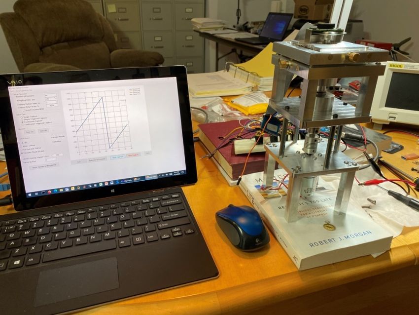
Photogrammetry Based PV Solutions Part V: Encoder Completion / TMS320F28379D
1 First Order of Business‐ AEAT‐9000 Optical Encoder Mount
This topic has haunted me now for much of 2020 as the first two design iterations proved less than
satisfactory to me. The second iteration is described in §5 for project completeness, but in the end I had
to move to yet a 3rd design iteration.
Although the 3rd iteration of the mechanical mount for the optical encoder is arguably over-kill, its
performance is excellent as is its repeatability and ease of alignment!
As mentioned at the end of §5, most of my performance difficulties would have probably been
solved had I moved to a single one-piece high quality 8 mm axle through the entire encoder mount, rather
than utilizing a 3/8” axle which was also turned down to 8mm for the encoder wheel. Leaving nothing to
chance, I also procured a much better axle for this design iteration. I also made notable improvements
with the bearings in this design iteration. However, since no cost-sensitive plans are in the forecast, it is
more important (to me) to have excellent performance with this 3rd design pass and be able to move on to
other aspects of my project rather than go through a cost reduction exercise now.
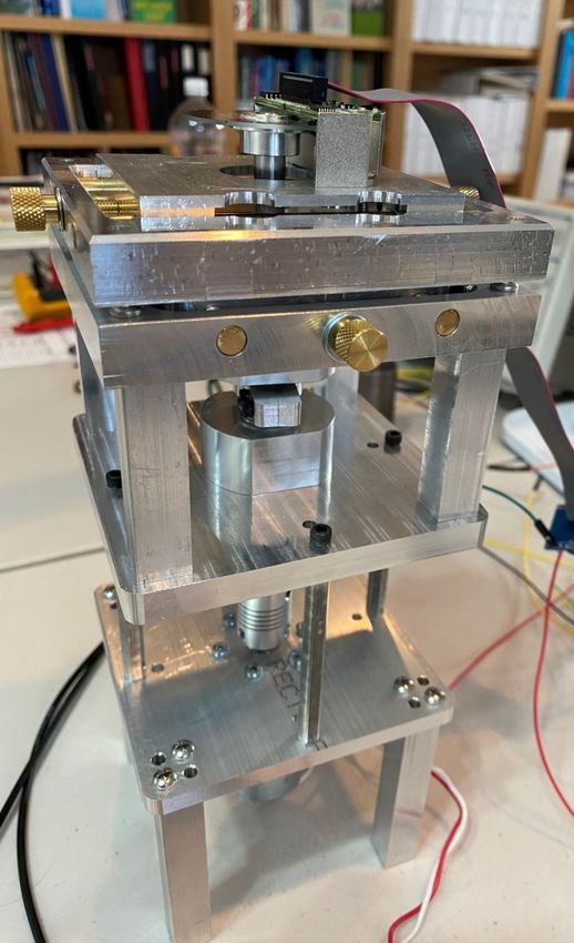
Two views of the final mechanical design are shown in Figure 1 and Figure 2.
Figure 1 Gen3 encoder mount employing precision x-y Figure 2 Secondary view of Figure 1
positioner
Copyright © 2017-2021 AM1 LLC 2 of 27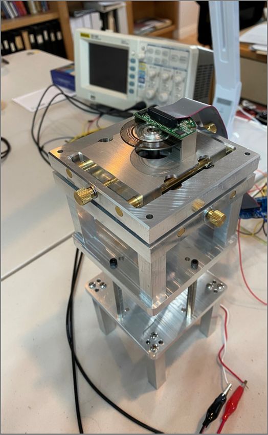
Photogrammetry Based PV Solutions                           Part V: Encoder Completion / TMS320F28379D

        The new encoder mount using the precision x-y positioner I designed and fabricated myself is
extremely easy to calibrate while also being rock solid and repeatable. Only the upper portion of the
stack-up will be used on each of the telescope axes since the bottom half (consisting of a 12V DC 100
RPM motor and coupling) is present only for initial x-y positioner alignment purposes.
        One of the major design objectives was to be able to align each optical encoder on this test jig,
and then be able to move it directly to the telescope axes without having to touch the alignment a second
time. By all indications, it looks like this objective has been achieved.
        A protective housing over the encoder wheel and associated electronics will have to be fabricated
of course to deal with environmental factors, but this design is otherwise completed and ready to move on
to the next phases in the project.

1.1 Baby Steps with the Arduino Mega2560 Platform
A C# graphical user interface (GUI) was written with a full command protocol for communications
between the PC and the Arduino Mega2560 which interfaces with the AEAT-9000 encoder. One of the
diagnostic screen shots from this program is shown in Figure 3. This aspect was originally discussed in
Part IV of this project story, but clean sawtooth behavior 1 was never really achieved because of the
performance issues associated with the encoder mount. With the new encoder mount, pristine sawtooth
behavior was always observed as shown in Figure 3.

Figure 3 16-bit absolute phase versus time from the encoder using a motor RPM value in the vicinity of
50. The ideal sawtooth wave is the result of a nearly constant RPM rate from the DC motor. A separate
diagnostic screen is used to examine the LSB behavior with no motor rotation applied.

1
  A constant motor RPM results in a constant angular velocity, and consequently a constant slope of the encoder
angle versus time.

Copyright AM1 LLC © 2017 - 2021                                                                        3 of 27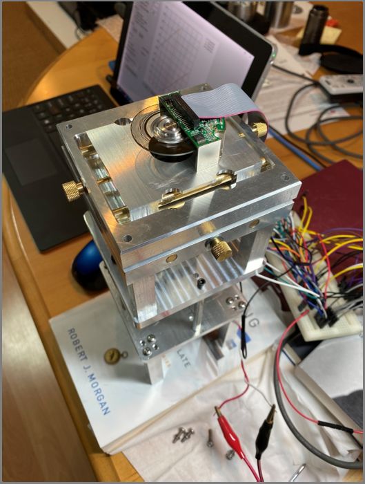
Photogrammetry Based PV Solutions Part V: Encoder Completion / TMS320F28379D
Figure 4 Wider perspective of encoder test jig operating with host PC and Arduino Mega
2 TMS320F28379D‐Centric Activities
Closure of the optical encoder mount design is finally enabling other aspects of this project to get
underway. A second encoder mount remains to be built and the two encoders physically integrated with
the telescope’s azimuth and elevation axes. Progress on the 25:1 torque enhancement block for the
elevation axis is nearing completion as well. Serious attention to the digital signal processing aspects of
the project is finally being given and the next steps described in §5 of [4] the previous project installment
pursued.
The near-term activities involving the DSP are sketched out in Figure 8. More specifically:
new C# graphical user interface (GUI) was written to support new phase of project
serial (asynchronous) communications between the host PC and DSP was developed, including a
new command protocol
serial communications between the DSP and optical encoder were developed based upon the
lessons learned using the Arduino Mega2560
control/interfacing between the DSP and its DRV8301 Booster Pack finished off the hardware
aspects for this installment
Many additional tasks remain to be accomplished of course, but the divide-and-conquer approach
outlined here was completed, with the next-steps described later in §3.
Copyright AM1 LLC © 2017 - 2021 4 of 27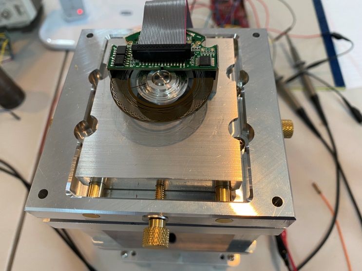
Photogrammetry Based PV Solutions                         Part V: Encoder Completion / TMS320F28379D

                                                                Figure 6 AEAT-9000 encoder and optical wheel.
                                                                (Mega2560 electronics)

Figure 5 Optical encoder, precision xy positioner, radial and
axial bearings, and test-jig low RPM motor. Only the top 1/3
of this assembly will be needed on each axle of the final
telescope mount. (Mega2560 electronics)

                                                                Figure 7 Side view of Figure 5. (Mega2560 electronics)

      Copyright AM1 LLC © 2017 - 2021                                                                   5 of 27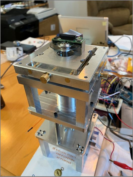
Photogrammetry Based PV Solutions                         Part V: Encoder Completion / TMS320F28379D

                                                    High-Speed
                                                    Serial Comm               AEAT-9000
                                                        (SPI)                  Encoder

                                                                                            3-Phase BLDC
     Host PC                   UART                                                             Motor
     C# GUI                 Serial Comm
                                (SCI)
                                                  TMS320F28379D                3-Phase
                                                   Core Algorithms              Motor
                                                                             Booster Pack

Figure 8 Major DSP elements involved with full motor control of one telescope axis2

2.1 Host PC GUI
The DSP must communicate with something during its related development so it is necessary to develop
the host PC software along in parallel. The splash screen for the host PC as presently working is shown
in Figure 9.
         The Diagnostics box in the lower right-hand corner will largely duplicate the functionality which
was previously implemented using the Arduino Mega2560 platform. The Telescope Alignment box in the
lower left-hand corner addresses future calibration activities of the telescope mount which will be done
against the night time background star field. A precision alignment method is crucial for the dual
telescope alignment, and was anticipated from the very beginning of the project [1].
         The Control diagnostics box middle-right will be the gateway into all of the brushless DC (BLDC)
motor control elements which have only been touched on to-date. In general, a large amount of effort will
be involved with each of the front-panel button functions, and these will be developed step by step as the
project progresses.

2
    From U27313 DSP Related.vsd.

Copyright AM1 LLC © 2017 - 2021                                                                    6 of 27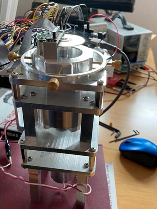
Photogrammetry Based PV Solutions                         Part V: Encoder Completion / TMS320F28379D

Figure 9 Splash screen for the new C# GUI

2.2 PC‐DSP Serial Communications
This communication occurs between the PC’s COM port and DSP’s UART (COM) port. The DSP’s SCI
resources are used to support this communication.
         Generally speaking, only one baud rate will be used. The port configuration is 8 data bits, 1 stop
bit, and no parity. Testing has been done for the this interface at several baud rates up to as high as
460.8 kbps with zero errors observed over a 12.5 hour period (14.871e6 characters or 118.97e6 bits). An
example screen shot of interface testing is shown in Figure 10. All communication via the COM port to the
DSP will be done using ASCII text strings. Data requested from the DSP by the PC will generally be
returned as 16-bit quantities using fixed formats.
         The PC-DSP Interface Diagnostics splash screen is shown in Figure 10. As noted in the caption,
extensive testing was done at 460.8 kbps with no errors observed. The speed for this interface needs to
be chosen in conjunction with activities conducted via the DSP’s SPI ports, however, to avoid excessive
interrupt collisions. To this end, the tentative baud rate used for PC-DSP communications is 57.6 kbps
whereas the baud rate used for SPI communications (with the AEAT-9000 optical encoders) is 4 Mbps.

Copyright AM1 LLC © 2017 - 2021                                                                    7 of 27
Photogrammetry Based PV Solutions                           Part V: Encoder Completion / TMS320F28379D

Figure 10 Screen shot of the PC-DSP interface undergoing test. Running at 460.8 kbps, no errors
observed over 12.5 hours and equivalently about 14.872 million characters3. String length is randomly
varied from 8 characters up to 60 characters in length. The baud rate for the PC-DSP interface has
tentatively been set at 57.6 kbps.

3
  SCI RXFIFO_RX2 for the interrupt, minimum string length = 1 character. Increasing FIFO interrupt level to RX8
(FIFO is 8/16 full before declaring interrupt) required a minimum string length of 10 characters.

Copyright AM1 LLC © 2017 - 2021                                                                        8 of 27

Photogrammetry Based PV Solutions Part V: Encoder Completion / TMS320F28379D
2.2.1 PC to DSP Commands
All commands to the DSP from the PC will be done using ASCII strings which are terminated in one null
character (0). Only the command string starting with “_X” is automatically echoed back from the DSP to
the PC.
A PC-to-DSP command consists of (i) a command name and (ii) up to 3 subsequent parameter
values all delineated by a white space. The command string must be terminated by a null character (0) as
already mentioned. The available commands are listed in Table 1.
Table 1 PC-to-DSP Commands
Command Description Parameter 1 Parameter 2 Parameter 3
$$$$ DSP reset
_reset_dsp DSP reset
Dummy message to be echoed
_X back to PC from 8 to 40 characters message
long
Set limits for azimuth axis range,
_set_az_limits +limit -limit
deg
Set limits for elevation axis range,
_set_el_limits +limit -limit
deg, relative to horizontal
_set_az_slew_limits Limit azimuth slew rate, deg/sec +limit -limit
_set_el_slew_limits Limit elevation slew rate, deg/sec +limit -limit
_reset_encoders Issue reset signal to encoders az reset el reset
Set 0o position for azimuth and or
_zero_encoders az true/false el true/false
elevation encoders
Start sampling action for azimuth
_enable_encoders az enable el enable
and or elevation encoders
Set sampling rate to be used by
_set_loop_fs fs
both control loops, sps
Set order (0,1,2) for azimuth and
_set_pwm_mash az value el value
elevation MASH - algorithm
Enable azimuth and or elevation
_enable_pwms az enable el enable
axis PWM
Set azimuth control loop
_set_az_pid_gains proportional, integral, and proportional integral differential
differential gains
Set elevation control loop
_set_el_pid_gains proportional, integral, and proportional integral differential
differential gains
Set up gain parameters for high-
_setup_az_hr_observer
rate azimuth encoder t observer
Set up gain parameters for low-
_setup_az_lr_observer
rate azimuth encoder t observer
Set up gain parameters for high-
_setup_el_hr_observer
rate azimuth encoder t observer
Set up gain parameters for low-
_setup_el_lr_observer
rate azimuth encoder t observer
Trap on encoder encountering
_encoder_location az_on el_on
location mark
Copyright AM1 LLC © 2017 - 2021 9 of 27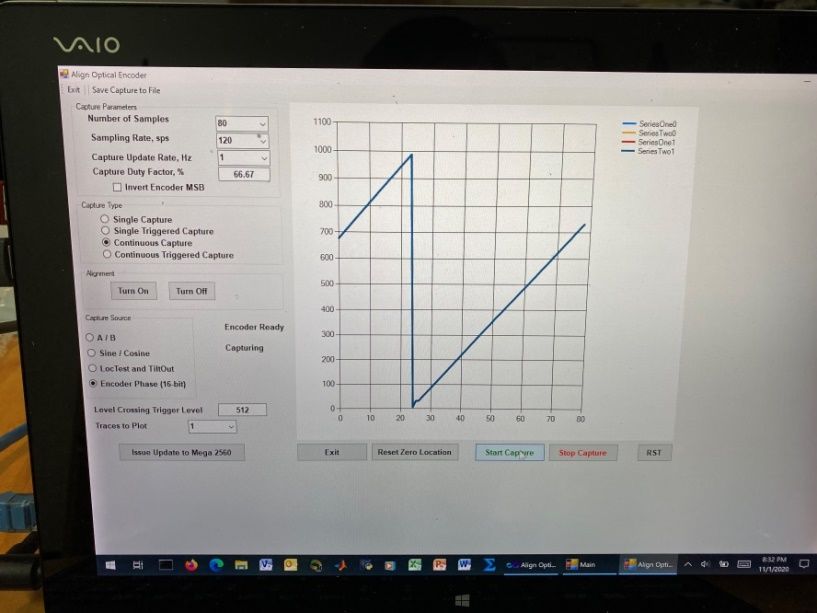
Photogrammetry Based PV Solutions Part V: Encoder Completion / TMS320F28379D
Command Description Parameter 1 Parameter 2 Parameter 3
Setup parameters for azimuth
_setup_az_pwm
PWM
Setup parameters for elevation
_setup_el_pwm
PWM
Setup to read parameters with
_setup_capture4 deci blk_size cap_type
decimation factor and block size
Initiate a capture (one-time) open_or_closed
_do_capture az_or_el
“a” for Az, “e” for El; “o” or “c” loop
_close_loops Close control loops, {t, f} az_loop el_loop
_step_az_axis Step azimuth axis given amount d
_step_el_axis Step elevation axis given amount d
Point telescope to specified az/el
_point_to az_angle el_angle
angles
Electrical interfacing details for operating the AEAT-9000 with the Arduino MEGA2560 were provided
in an earlier report [4]. These interfacing details are repeated here for convenience in Table 3 of §5. Only
a subset of these signals can be supported in the full-up DSP version supporting full servo control
because (i) the DRV8301 Booster Pack (which will drive the two 3-phase motors) will take up a large
number of I/O pins and (ii) two optical encoders need to be supported as well. Two configurations were
used for this portion of the project:
Configuration 1: Run the TMS320F28379D without the DRV8301’s present to free up more
GPIO pins for general I/O. This configuration supported all of the functionality provided in the
Arduino version.
Configuration 2: Install the DRV8301 Booster Packs on the DSP, and retain as much of the
1st configuration functionality as possible. With only one DRV8301 installed, all of the 1st
configuration functionality has been retained.
2.2.2 SCI Interface (DSP PC)
The F28379D’s SCIA interface is used for communications between the PC and DSP. The baud rate for
this interface should not be chosen independently of the encoder sampling rate because the SCI interface
can only be serviced / checked at this sampling rate. If the encoder sampling rate is too low and the SCI
baud rate too high, the SCIA FIFO may be overrun. Tentatively:
SCI baud rate = 57.6 kbps
SPI baud rate = 4 Mbps
Encoder sampling rate= 8 kHz to 160 kHz5
All communications from the PC to the DSP are ASCII strings. Data returned from the DSP is,
however, functionally dependent and generally binary in nature to conserve throughput. Blocks of data
associated with the encoders’ angular position or (I, Q) signals are sent back from the DSP to the PC
upon command. These quantities are always sent as 16-bit signed integer quantities.
4
0: do nothing, 1: open-loop, angle data; 2: open-loop, I/Q data; 3: closed-loop
5
This rate easily supported without closed-loop calculations included yet. This high rate does demonstrate, however,
the proficiency of the optical encoder and DSP-encoder interface routines.
Copyright AM1 LLC © 2017 - 2021 10 of 27Photogrammetry Based PV Solutions Part V: Encoder Completion / TMS320F28379D
2.2.3 Dedicated GPIO (DSP Encoder)
The optical encoders (AEAT-9000) require several dedicated control signals from the DSP aside from the
SPI interface. Port SPIA is dedicated to azimuth operations and SPIB will be dedicated to elevation
operations.
Table 2 DSP AEAT-9000 Encoder Interface. Full (I/Q) support is only shown for the azimuth channel.
DSP Signal DSP GPIO DSP Pin Encoder Flex-Cable
Name Signal Name Pin
SPIACLKA 60 J1-7 SCL 28
SPISIMOA 58 J2-15
SPISOMIA 59 J2-14 Dout+ 22
SPISTEA 61 J2-19 NSL 14
ZRSTA 122 J2-17 zero_Reset 12
nRSTA 123 J2-18 nRST 26
COSINEAP ADCINA0 J3-30 COSINE+ 1
COSINEAN ADCINB2 J3-28 COSINE- 2
SINEAP ADCINC3 J3-24 SINE+ 3
SINEAN ADCIN14 J3-23 SINE- 4
SPIACLKB 65 J5-47 SCL
SPISIMOB 63 J6-55
SPISOMIB 64 J6-54 Dout+
SPISTEB 66 J6-59 NSL
ZRSTB zero_Reset
nRSTB nRST
+5VA J3-21 27, 29
GNDA J3-22 6, 8, 17, 18
+5VB J7-61
GNDB J7-62
One issue did come up in formulating the interface details shown in Table 2. Although the AEAT-
9000 datasheet clearly stated SCL- and NSL- signal inputs can be tied to fixed rail voltages and the
device operated effectively single-ended, this was not the case. In order for proper operation to occur,
SCL- and NSL- signals had to be tied to approximately VCC/2.
Once each encoder is installed into the telescope mount, only 3-wires (plus power and ground)
should be required to communicate with the AEAT-9000’s as highlighted in bold-blue Flex-Cable Pin
numbers as shown in the table.
The SPI configuration adopted (from CodeComposer) is given by
SPI_setConfig(SPIA_BASE, DEVICE_LSPCLK_FREQ, SPI_PROT_POL1PHA0,
SPI_MODE_MASTER, 4000000, 16);
SPI_disableLoopback(SPIA_BASE);
SPI_setEmulationMode(SPIA_BASE, SPI_EMULATION_STOP_AFTER_TRANSMIT);
This information provides the polarity and phasing used for the 3-wire interfacing, along with the 4 Mbps
baud rate and 16-bits per word details.
Copyright AM1 LLC © 2017 - 2021 11 of 27Photogrammetry Based PV Solutions Part V: Encoder Completion / TMS320F28379D Figure 11 Encoder phase versus time plot for constant RPM case Figure 12 Analog interpolation using quadrature waveforms is used within the decoder to extend angular resolution from 11-bits to 17-bits. The constellation plot assists with the fine-alignment step.IQ sample values should fall along the perimeter of a best-fit circle as shown here in the right-hand plot. Copyright AM1 LLC © 2017 - 2021 12 of 27
Photogrammetry Based PV Solutions                             Part V: Encoder Completion / TMS320F28379D

Figure 13 Same6 as Figure 12 except encoder sampling rate increased from 12.5 kHz to 160 ksps using
a post-sampling decimation factor of 2

         Figure 12 and Figure 13 provide some insight into how well the optical encoder is aligned. Since
the optical encoders will primarily be utilized for estimating position (thereby entailing essentially zero
radian frequency), the quality of the signal I,Q constellation versus angle is what is of greatest interest.
This information can only be obtained by using a fairly high encoder sampling rate and from which this
perspective is stitched together.
         The slowest rotational rate my nominal 100 RPM motor can spin at without stalling is roughly 30
RPM. One cycle of the interpolating I,Q sinewaves occurs between each of the 2048 ticks on the encoder
wheel. Consequently, the sinewave frequency at this lowest RPM rate is on the order of (30/60)*2048 =
1024 Hz. Therefore, an encoder sampling rate of at least 32,768 sps is required in order to have roughly
32 samples per sinewave period.
         Different encoder sampling rates combined with different sample buffer depths can be used to
explore the numerical precision of the encoder’s performance. As described in §8, a constant angular
velocity presumption is made. Several known encoder wheel imperfections are known to be present and
these are manifested as larger spikes in Figure 14 and Figure 15. The RMS error (relative to a straight
line) appears to be independent of the sample rate and capture window width. The encoder is known to
be extremely sensitive so the RMS floor of about 12 LSBs is presently believed to be due to angular
roughness of the (very inexpensive) low RPM motor since it has a substantial gear-reduction train built in.
This assumption remains to be proven/disproven by other means.

6
   The AEAT-9000 creates the last 6-bits or resolution using analog interpolation of in-phase and quadrature-phase
signals. This 90o relationship can be seen in the left-hand graphic of the figure.

Copyright AM1 LLC © 2017 - 2021                                                                          13 of 27
Photogrammetry Based PV Solutions Part V: Encoder Completion / TMS320F28379D Figure 14 Decimated sampling rate of 40 ksps with sample capture interval of about 0.8 msec Figure 15 Decimated sampling rate of 5 ksps with sample capture interval of about 6.4 msec Copyright AM1 LLC © 2017 - 2021 14 of 27
Photogrammetry Based PV Solutions Part V: Encoder Completion / TMS320F28379D 2.3 Texas Instruments DRV8301 BLDC Motor Booster Pack The Texas Instruments DRV8301 Booster Pack was easily installed atop the TMS320F28379D Launchpad. The DRV8301 provides 3.3V to the Launchpad, and a switcher on the Launchpad is used to create 5V for the Launchpad as well as the AEAT-9000 optical encoder. Jumpers had to be changed on the Launchpad as: Remover jumpers JP1, JP2, and JP3 Install jumper JP6 The results shown in Figure 13 were taken with the hardware configured with the Booster Pack as discussed herein and shown in Figure 16. Figure 16 DRV8301 Booster Pack installed atop the TMS320F28379D Launchpad XL DSP board. The twisted red-white pair bring in +12V whereas other voltages (3.3V and 5V) are created internally. Copyright AM1 LLC © 2017 - 2021 15 of 27
Photogrammetry Based PV Solutions Part V: Encoder Completion / TMS320F28379D
3 Next Steps
Both hardware and software elements remain to be developed. With the encoder mounting now solved,
there do not appear to be any major obstacles ahead on the hardware side (aside from possibly
configuring the second DRV8301 atop the Launchpad XL and having sufficient IO).
On the software side, however, a great deal of work remains to be done. At this juncture, the
most tedious appears to be proper configuration and usage of the ePWM blocks which are used to drive
the 3-phase motors. The concepts involved are not difficult, but a fair amount of tedium is expected in
getting the end-results to match expectations.
3.1 Near‐Term Hardware Efforts
Fabricate at least 2 more encoder mounts
Design and fabricate test jig modification to replace 100 RPM motor with small 3-phase DC motor
(planned for elevation axis less 25:1 pulley module) for algorithm development
Design and fabricate encoder mount to azimuth axis assembly
Complete the elevation 25:1 pulley module
3.2 Near‐Term Software Efforts
Become familiar with ePWM modules including all limit/safety features
Become familiar with built-in control loop accelerator hardware (CLA) within the F28379D
Code a first-cut rudimentary control loop
4 References
1. J.A. Crawford, “Photogrammetry for Non-Invasive Terrestrial Position/Velocity Measurement of
High-Flying Aircraft,” Part I, 16 Oct. 2017, U24866.
2. ___________, “Photogrammetry for Non-Invasive Terrestrial Position/Velocity Measurement of
High-Flying Aircraft, Direct-Drive Motors,” Part II, 23 April 2019, U24933.
3. ___________, “Photogrammetry for Non-Invasive Terrestrial Position/Velocity Measurement of
High-Flying Aircraft, Direct-Drive Motor Chassis Design & Assembly,” Part III, 12 Nov 2019,
U24933.
4. ___________, “Photogrammetry for Non-Invasive Terrestrial Position/Velocity Measurement of
High-Flying Aircraft, Optical Encoder & Elevation Drive,” Part IV, 23 Aug 2020, U24933.
5. ____________, Advanced Phase-Lock Applications- Synthesis, Chapter 5, unpublished.
Copyright AM1 LLC © 2017 - 2021 16 of 27Photogrammetry Based PV Solutions Part V: Encoder Completion / TMS320F28379D
5 Appendix: Optical Encoder Work‐ 2nd Iteration
Work on the optical encoder (Broadcom AEAT-9000) has continued in the installment of the project.
Unfortunately, this encoder was obsoleted by Broadcom mid-2020, but because its claimed 17-bit single-
rotation precision is rather unique in the industry at this price-point, I decided to make a lifetime buy of
devices for myself and press forward. Other encoders are available in the marketplace, but at a
substantially higher price-tag (6x and higher).
Although the two-thumbwheel alignment concept from Part IV should have been sufficient
conceptually speaking, device alignment proved to be almost impossible because this approach co-
mingled x-axis and y-axis corrections. Not surprisingly, literally everything matters when it comes to
getting the advertised performance from the device. Notably:
rotational axis concentricity must be extremely good ( better than 0.001”) for the code wheel.
vertical positioning of the codewheel between the AEAT9000’s built-in LED and supporting
sensors has been found to be very critical as well.
x-dimension and y-dimension positioning must be rock solid, delivering consistent positioning with
an accuracy (after alignment) on the order of 0.001”
I built a new-and-improved optical encoder alignment jig at the beginning of this project installment as
shown in Figure 17
Encoder on
adjustment sled
Dual bearings
Fly wheel
100 RPM motor
Figure 17 Revised optical encoder alignment-test jig
Copyright AM1 LLC © 2017 - 2021 17 of 27Photogrammetry Based PV Solutions Part V: Encoder Completion / TMS320F28379D
Figure 18 AEAT9000 optical encoder mounted on Figure 19 Sled situated in adjustment housing
sled
Figure 20 Milled housing for dual bearings Figure 21 Housing with dual bearing installed-
milled to a precision of about 0.0005”
Figure 22 Encoder, sled, adjustment housing and Figure 23 Motor mounting plate
dual bearings assembled together
Copyright AM1 LLC © 2017 - 2021 18 of 27Photogrammetry Based PV Solutions Part V: Encoder Completion / TMS320F28379D
Two additional photos of the completed alignment jig are shown in Figure 24 and Figure 25. I reached
several other conclusions using this improved calibration jig:
Even though I turned the axle on my lathe to a concentricity better than a few thousandths of an
inch, I found the sloppiness in the bearings and axle-related concentricity still came through and
resulted in an unacceptable amount of wobble.
Bearing arrangement must address all three dimensions as already mentioned.
A flex-coupling is probably recommended between the optical encoder assembly’s rotational axis
and the end application
Precision alignment of the stand-alone assembled optical encoder should take place first,
followed by mating of the assembly to the final application. Otherwise, in-situ alignment could be
problematic.
Using the 6-32 thumbscrews for x-y adjustment could probably have worked even with the
backlash and poor rigidity during adjustment, but hoping to avoid yet another design iteration in
the future, a better approach is needed.
The exercise did validate the AEAT-9000’S claimed achievable performance at least to a degree.
Mechanical integrity must still be improved, however, before a complete victory can be declared.
Figure 24 Top-view of alignment jig in action
Figure 25 Side-view of alignment jig in action
Moving to the next level, I took the following steps:
1. Purchase high-precision bearings and axle components from McMaster-Carr.
2. Rather than use a 3/8” rod and have to turn the diameter down to 8mm to fit the code wheel’s
inner diameter, opt to use a 8mm diameter rod throughout the stand-alone optical encoder
assembly.
3. A flexible coupler should be used to mate the stand-alone optical encoder assembly to its final
application.
4. A much more rigid reproducible design for the x-y plane adjustments needs to be used.
Copyright AM1 LLC © 2017 - 2021 19 of 27Photogrammetry Based PV Solutions Part V: Encoder Completion / TMS320F28379D
Table 3 Optical Encoder I/O Mapping from AEAT-9000 to Arduino MEGA2560 [4] (Pin # refers to the flex
cable wire index)
Encoder Pin Pin Mega 2560 Pin Dig/Ana Mega Comments
Name # Name I/O
COSINE+ 1 A0 A I Truly differential
COSINE- 2 A1 A I Truly differential
SINE+ 3 A2 A I Truly differential
SINE- 4 A3 A I Truly differential
TiltOut Used for encoder/wheel tilt alignment.
5 22 D I
Two pulses per encoder revolution.
GND 6 Hard to GND
LocTest 7 A4 A I Used for radial code wheel alignment
GND 8 Hard to GND
Not Used 9 ---
MSBINV 10 23 D O
SPI_CLK 11 24 D O
Zero_RST 12 25 D O
SPI_SI 13 26 D O
NSL+ Connect to GND before encoder is
14 50 D O
powered on
SPI_SO 15 27 D I
Connect to VDD before encoder is
NSL- 16 48
powered on
GND 17 Hard to GND
GND 18 Hard to GND
INCB 19 30 D I
DOUT- 20 47 D I
INCA 21 32 D I
DOUT+ 22 33 D I
DIN- 23 38 D O
LERR 24 39 D I
DIN+ 25 40 D O
nRST 26 41 D O Encoder reset
VDD 27 5V PWR
SCL+ 28 42 D O
VDD 29 5V PWR
SCL- 30 43 D O
Copyright AM1 LLC © 2017 - 2021 20 of 27Photogrammetry Based PV Solutions Part V: Encoder Completion / TMS320F28379D
6 Appendix: Signal Observer
The DSP signal observer blocks perform filtering and signal conditioning within the system. The topic was
first introduced in §4.1 of [2]. The observer’s behavior is governed by two parameters denoted by and .
The DSP design makes use of low-rate and high-rate observer functions which are identical
except for the ( , ) parameter values used. The high-rate observer block will generally be used within
the control loops where additional signal delay must be kept to a minimum. The low-rate observer blocks
are intended for use when monitoring of the system’s behavior is of interest and the observer output is
decimated down to rates on the order of 100 sps or less.
7 Appendix: 3‐Phase Interpolation Algorithms
Unlike most motor control algorithms in the literature, I need to have very precise (e.g., 10 arc-second)
precision pointing making jitter or wandering of either axis critical concerns. Since the associated
algorithms must be executed at the sampling rate (i.e., perhaps as high as 160 ksps), execution efficiency
is critical as well. Making use of the build-in CLA’s within the F28379D should help ease memory as well
as execution resource concerns.
For 3-phase control, the voltage waveforms given by
VA AA sin
4 3 1
VB AB sin AB cos sin (1)
3 2 2
4 3 1
VC AC sin AC cos sin
3 2 2
must be efficiently computed. A sine (and cosine) table of sufficiently small granularity along with
numerical interpolation is the most economical way to proceed. The 2nd order interpolation method
developed in [5] approximates the in-phase and quadrature-phase terms as7
2
I ~ I table 1 Qtable
2
(2)
2
Q Qtable 1 I table
2
where the angle of interest is given by k where the angular step between table look-up
values is given by and / 2 . Interpolated performance using (2) versus ideal are shown in
Figure 26 through Figure 31 for an effective table lookup length8 of 160.
7
Ideally, I cos and Q sin .
8
Due to symmetry arguments, the physical lookup table length needs to only be 1/8 of the effective table length.
Copyright AM1 LLC © 2017 - 2021 21 of 27Photogrammetry Based PV Solutions Part V: Encoder Completion / TMS320F28379D
x 10
-6 I & Q Voltage Error vs Angle
1.5
1
0.5
Ierr | Qerr
0
-0.5
-1
Lookup Table Size= 160
-1.5
0 50 100 150 200 250 300 350 400
Axis Angle, deg
Figure 26 In-phase and quadrature-phase errors
x 10
-6 I & Q Voltage Error vs Angle
1
0.5
Ierr | Qerr
0
-0.5
-1
Lookup Table Size= 160
-1.5
64 65 66 67 68 69 70
Axis Angle, deg
Figure 27 Close-up of Figure 26
Copyright AM1 LLC © 2017 - 2021 22 of 27Photogrammetry Based PV Solutions Part V: Encoder Completion / TMS320F28379D
x 10
-6 Amplitude Error vs Angle
1.4
1.2
1
Amplitude Error, V
0.8
0.6
0.4
0.2
Lookup Table Size= 160
0
0 50 100 150 200 250 300 350 400
Angle, deg
Figure 28 Amplitude error
x 10
-7 Amplitude Error vs Angle
12
10
Amplitude Error, V
8
6
4
2 Lookup Table Size= 160
0
50 52 54 56 58
Angle, deg
Figure 29 Close-up of Figure 28
Copyright AM1 LLC © 2017 - 2021 23 of 27Photogrammetry Based PV Solutions Part V: Encoder Completion / TMS320F28379D
Phase Error vs True Angle
0.3
0.2
0.1
Error, Arc-Sec
0
-0.1
-0.2
-0.3
Lookup Table Size= 160
-0.4
0 50 100 150 200 250 300 350 400
Angle, deg
Figure 30 Phase error
Phase Error vs True Angle
0.2
0.1
Error, Arc-Sec
0
-0.1
-0.2 Lookup Table Size= 160
-0.3
54 56 58 60 62 64
Angle, deg
Figure 31 Close-up of Figure 30
Copyright AM1 LLC © 2017 - 2021 24 of 27Photogrammetry Based PV Solutions Part V: Encoder Completion / TMS320F28379D
Table 4 Interpolation Error Performance vs Table Lookup Size
Effective Lookup Pk-Pk Amplitude Error, Pk-Pk Phase Error,
Table Size V Arc-Seconds
64 1.97e-5 8.13
128 2.46e-6 1.02
160 1.26e-6 0.52
192 7.30e-6 0.298
256 3.08e-7 0.127
Copyright AM1 LLC © 2017 - 2021 25 of 27Photogrammetry Based PV Solutions Part V: Encoder Completion / TMS320F28379D
8 Appendix: IQ Constellation Fidelity & Encoder Precision
As described briefly in §2.2.3, the AEAT-9000 optical encoder delivers 11-bit resolution using Gray-
encoded tracks and interpolates the remaining 6-bits using I/Q analog signal interpolation on-chip. The
analog I/Q signals are conveyed to the DSP’s built-in ADCs and it is these digitized I/Q signals being
plotted in Figure 12 and Figure 13. Although the AEAT-9000 datasheet claims that much of the device
calibration is done in the factory, an all but undocumented calibration mode is also provided for the device
user. It is therefore difficult at best to know the final details with certainty.
If the analog I/Q signals from the AEAT-9000 truly represent the internal state of affairs within the
encoder, constellation points are expected to fall onto an ellipse which may also be rotated as well as
offset from the origin. An ideal ellipse in the x, y plane is given by9
x2 y 2
1 (3)
a 2 b2
where the major axis is given by 2a, the minor axis is given by 2b, and eccentricity is given by e c / a
along with
c a 2 b2 (4)
Consequently, the eccentricity is also given by
2
c a 2 b2 b
e 1 (5)
a a a
A diagram illustrating the different quantities is provided in Figure 32.
0,b
d1 d2
c, 0 c, 0 a, 0
Figure 32 Classic ellipse
If the ellipse (3) is rotated by angle and then offset by x, y , (3) is transformed to
9
College Calculus with Analytic Geometry, Protter & Morrey, 1970, page 303.
Copyright AM1 LLC © 2017 - 2021 26 of 27Photogrammetry Based PV Solutions Part V: Encoder Completion / TMS320F28379D
x cos y sin x y cos x sin y
2 2
2
1 (6)
a b2
Working in reverse with a set of constellation x, y points, the best-fit ellipse in terms of a, b, ,
x , and y is now sought. An error function can be defined as
2
xk cos yk sin x yk cos xk sin y
2 2
K
1 (7)
k 1 a2 b2
and the estimation parameters identified which minimizes this function. Subsequent calculations may be
somewhat simplified by choosing a modified form of (7) as
K 2
m b 2 xk cos yk sin x a 2 yk cos xk sin y a 2b 2
2 2
(8)
k 1
This is still too complicated to be used effectively, especially when there will be 2048 interpolation periods
involved for the entire encoder wheel. Rather, only a goodness of alignment metric (GAM) is being sought
from which to guide the encoder’s x/y alignment with the axis of rotation. In this respect, a goodness of fit
to an ideal circle should be sufficient.
Since the overall control loops will only be making use of the 16-bit digital encoder output, it
makes sense to focus the encoder alignment metric on using this output alone. To this end, several
assumptions can be made:
Alignment activities can be done using the DC motor at about 30 RPM, but no lower with the
present motor.
At 30 RPM, the rotation rate is about 0.5 turn per second, resulting in about 1024 I/Q cycles per
second.
At an encoder sampling rate of 160 ksps and capture depth of 200 (I/Q) samples, each capture
will encompass only about 1.25 msec and equivalently about one full cycle of the I/Q waveforms.
Over time intervals of 1.25 msec, mechanical inertia should keep the rotational rate constant even
if the motor has some variations (which it no doubt will).
o The encoder sampling rate can likely be lowered by a factor of 4 to encompass 4
complete I/Q signal cycles without compromising this constant rate assumption.
Under these assumptions, the GAM can be computed for all 2048/4 = 512 segments of the encoder
wheel and used to physically align the optical encoder to the axis center as best as possible. If this does
still not produce sufficient encoder fidelity, additional compensation methods based upon axle angle will
have to be considered.
The GAM for each sample capture will be computed as follows using only the encoder’s 16-bit
outputs:
1. Estimate the axle’s angle corresponding to the center of the capture time. With the constant
angular velocity assumption, this is straight forward to do.
2. In a similar fashion, estimate the constant angular velocity present for the capture.
3. Ideally, the angle samples will fall on a straight line. The RMS deviation of samples from the
straight line will be the GAM value corresponding to that axle’s center position.
4. Subsequent captures are performed until the entire 360o of axle angle travel is characterized in
this fashion.
Copyright AM1 LLC © 2017 - 2021 27 of 27You can also read