Process noise distinguishes between indistinguishable population dynamics - bioRxiv
←
→
Page content transcription
If your browser does not render page correctly, please read the page content below

bioRxiv preprint first posted online Jan. 29, 2019; doi: http://dx.doi.org/10.1101/533182. The copyright holder for this preprint
 (which was not peer-reviewed) is the author/funder, who has granted bioRxiv a license to display the preprint in perpetuity.
                                    All rights reserved. No reuse allowed without permission.

       Process noise distinguishes between indistinguishable
                                              population dynamics

      Matthew J. Simpson* 1 , Jacob M. Ryan1 , James M. McGree1,2 , and Ruth
                                                               E. Baker3

      1
          School of Mathematical Sciences, Queensland University of Technology
                              (QUT), Brisbane, Queensland 4001, Australia
        2
            ARC Centre of Excellence for Mathematical and Statistical Frontiers,
                                                         QUT, Australia.
             3
                 Mathematical Institute, University of Oxford, Oxford, OX2 6GG,
                                                        United Kingdom

                                                        January 29, 2019

                                                                Abstract

                    Model selection is becoming increasingly important in mathematical biology.
                 Model selection often involves comparing a set of observations with predictions
                 from a suite of continuum mathematical models and selecting the model that pro-
                 vides the best explanation of the data. In this work we consider the more challeng-
                 ing problem of model selection in a stochastic setting. We consider five different
                 stochastic models describing population growth. Through simulation we show that
                 all five stochastic models gives rise to classical logistic growth in the limit where we
                 consider a large number of identically prepared realisations. Therefore, comparing
          * To   whom correspondence should be addressed. E-mail: matthew.simpson@qut.edu.au

                                                                       1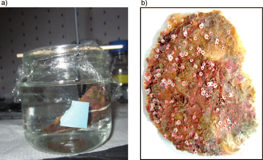
bioRxiv preprint first posted online Jan. 29, 2019; doi: http://dx.doi.org/10.1101/533182. The copyright holder for this preprint
 (which was not peer-reviewed) is the author/funder, who has granted bioRxiv a license to display the preprint in perpetuity.
                                    All rights reserved. No reuse allowed without permission.

              mean data from each of the models gives indistinguishable predictions and model
              selection based on population-level information is impossible. To overcome this
              challenge we extract process noise from individual realisations of each model and
              identify properties in the process noise that differ between the various stochastic
              models. Using a Bayesian framework, we show how process noise can be used suc-
              cessfully to make a probabilistic distinction between the various stochastic models.
              The relative success of this approach depends upon the identification of appropri-
              ate summary statistics and we illustrate how increasingly sophisticated summary
              statistics can lead to improved model selection, but this improvement comes at the
              cost of requiring more detailed summary statistics.

     Keywords: logistic growth; model selection; population dynamics

                                                                       2
bioRxiv preprint first posted online Jan. 29, 2019; doi: http://dx.doi.org/10.1101/533182. The copyright holder for this preprint
 (which was not peer-reviewed) is the author/funder, who has granted bioRxiv a license to display the preprint in perpetuity.
                                    All rights reserved. No reuse allowed without permission.

     1        Introduction

     The logistic growth equation,

                                                   dC(t)             C(t)
                                                         = λC(t) 1 −        ,                                                       (1)
                                                    dt                K

     with solution,
                                                                   KC(0)
                                                C(t) =                            ,                                                 (2)
                                                           C(0) + e−λt (K − C(0))
     is probably the most widely used model of population dynamics in the fields of mathe-
     matical biology and mathematical ecology (Edelstein-Keshet 2005; Murray 2002). In this
     continuum framework, C(t) ≥ 0 is the number, or number density, of individuals, λ > 0
     is the low-density growth rate and K > 0 is the carrying capacity of the environment.
     The key feature of the logistic growth model is that when the initial population density
     is small compared to the carrying capacity, C(0)/K  1, the solution takes the form of a
     sigmoid curve that monotonically increases from C(0) and asymptotes to lim C(t) = K − .
                                                                                                                  t→∞

          For small initial densities, C(0)/K  1, the logistic growth model can be approxi-
     mated by a simpler exponential growth model since C(t) ∼ C(0)eλt for sufficiently small
     t (Warne et al. 2017). In the exponential growth model, the per capita growth rate is a
     positive constant, (dC(t)/dt)(1/C(t)) = λ, that is independent of the population den-
     sity. This feature leads to unbounded growth as t increases. In contrast, the per capita
     growth rate for the logistic model, (dC(t)/dt)(1/C(t)) = λ[1 − C(t)/K], is a linearly
     decreasing function of C(t), such that the per capita growth rate is zero at C(t) = K,
     which leads to bounded populations at large time. This kind of transition between low-
     density exponential growth and high-density saturation are the two key elements of the
     logistic growth model that make it so appealing since these features are widely observed
     in many applications in biology and ecology (Edelstein-Keshet 2005; Murray 2002).

          In a biological context, images in Figure 1(a)-(b) show the growth of a population of
     prostate cancer cells in two-dimensional cell culture at t = 0 and t = 48 h, respectively
     (Jin et al. 2016). This kind of growth process becomes limited by available space in the
     monolayer as the density increases, as illustrated in Figure 1(c). This reduced growth rate
     at larger densities is often modelled using Equations (1)-(2) (Browning et al. 2018; Cai

                                                                       3
bioRxiv preprint first posted online Jan. 29, 2019; doi: http://dx.doi.org/10.1101/533182. The copyright holder for this preprint
 (which was not peer-reviewed) is the author/funder, who has granted bioRxiv a license to display the preprint in perpetuity.
                                    All rights reserved. No reuse allowed without permission.

     et al. 2007; Sengers et al. 2007; Tremel et al. 2009). In an ecological context, the image
     in Figure 1(d) shows a population of polyps growing on the surface of an oyster shell.
     Similar to the population of cells in Figure 1(a)-(b), the net growth rate of the polyps
     reduces as the density increases, as illustrated in Figure 1(e). This kind of saturation can
     be accurately predicted using the logistic growth model (Melica et al. 2014) as illustrated
     in Figure 1(e). Many other kinds of ecological growth processes, such as populations of
     plants, are also modelled using Equations (1)-(2) (Bolker and Pacala 1997; Law et al.
     2003). Far more complicated organism-level growth phenomena also exhibit saturation
     behaviour as illustrated by images in Figure 1(f)-(g) showing the growth of a Shiba Inu
     puppy at age 12 and 30 weeks, respectively. The time series showing the weight of the
     puppy, given in Figure 1(h), takes the form of a sigmoid curve that can be modelled
     using Equations (1)-(2). We note, however, that while whole organism-level growth can
     be approximately modelled using the classical logistic equation, as illustrated in Figure
     1(h), other generalised logistic growth laws are often used to study organism-level growth
     (Frascoli et al. 2014; Goriely 2017; Tsoularis and Wallace 2002).

          Instead of working with a continuum-level description of population dynamics, such
     as Equations (1)-(2), it is often the case in mathematical biology and mathematical
     ecology that stochastic discrete models are used (Bolker and Pacala, 1997; Codling et
     al. 2008; Ermentrout and Edelstein-Keshet 1993; Lambert et al. 2018; Law et al. 2003;
     Maclaren et al. 2015). Individual-based stochastic models are sometimes preferred over
     continuum models since continuum models can not provide information about individual-
     level behaviour and continuum models do not capture or predict stochastically (Frascoli
     et al. 2013; Treloar et al. 2014; O’Dea and King 2012).

          In this section we describe five different discrete models of population dynamics and
     explain their relationship to Equations (1)-(2). In our description of these models we
     pay careful attention to illustrate the different mechanisms inherent in each model, and
     we describe how each model can be simulated to produce stochastic realisations. Using
     results of these stochastic realisations, we demonstrate that each of the different discrete
     models gives rise to indistinguishable logistic growth in the limit of a very large number
     of identically prepared realisations. Therefore, when we are dealing with noisy individual
     realisations of the discrete models we are considering random variables. In contrast, when

                                                                       4
bioRxiv preprint first posted online Jan. 29, 2019; doi: http://dx.doi.org/10.1101/533182. The copyright holder for this preprint
(which was not peer-reviewed) is the author/funder, who has granted bioRxiv a license to display the preprint in perpetuity.
All rights reserved. No reuse allowed without permission.
0.002
C(t) [cells/mm2]
0.001
0 24 48 72 96
(a) (b) (c) t [h]
C(t) [polyps/cm2]
(d) (e) t [days]
10
8
W(t) [kg]
6
4
2
0
(f) (g) (h) 0 10 20 30 40
t [weeks]
Figure 1: Examples of logistic growth-type phenomena. (a)-(b) shows images of a
cell proliferation assay performed with prostate cancer cells [23]. The images in (a) and
(b) correspond to t = 0 and t = 48 h, respectively, and each image shows a region that
is approximately 450 µm2 in area. The plot in (c) shows experimental estimates of cell
density, C(t), (red crosses) superimposed on a plot of Equation (2) with C(0) = 0.001
cells/µm2 , K = 0.002 cells/µm2 and λ = 0.04 /h. (d) shows an oyster shell, upon which
a population of polys (red) are growing. The plot in (e) shows experimental estimates
of the polyp density, C(t), superimposed on a plot of Equation (2) with C(0) = 0.081
polyps/cm2 , K = 1.81 polyps/cm2 and λ = 0.006 /h. Images in (f) and (g) show
photographs of a Shiba Inu puppy Frankie, aged 12 and 35 weeks, respectively. Data in
(h) show time series measurements of Frankie’s weight, w(t) (red dots) superimposed on
a plot of Equation (2) with C(0) = 0.35 kg, K = 10.7 kg and λ = 0.00113 /h. Images
and data in (a)-(c) are reproduced with permission from Jin et al. (2016). Images and
data in (d)-(e) are reproduced with permission from Melica et al. (2014). Images in (f)
and (g), and data in (h) were obtained by the first author.
5bioRxiv preprint first posted online Jan. 29, 2019; doi: http://dx.doi.org/10.1101/533182. The copyright holder for this preprint
(which was not peer-reviewed) is the author/funder, who has granted bioRxiv a license to display the preprint in perpetuity.
All rights reserved. No reuse allowed without permission.
we consider the averaged outcome of a large number of identically prepared realisations of
the discrete models we are dealing with deterministic variables. To make this distinction
clear we denote the number of individuals in any realisation from any one of the five
discrete models as C(t), and the average number of individuals constructed using a large
number of identically prepared realisations as
N
1 X
hC(t)i = Cn (t), (3)
N n=1
where Cn (t) is the number individuals in the nth identically prepared realisation of a
particular stochastic model at time t, and N is the total number of realisations used to
construct the averaged density.
2 Discrete models
We will now describe and implement the five completely distinct stochastic models that
we consider in this work. The first three models are spatially implicit models meaning
that we consider the population of individuals as being spatially well-mixed but we do
not explicitly consider the spatial location of any particular individual (Geritz and Kisdi,
2012). In contrast, the last two models are spatially explicit and we explicitly track
the position of each individual within the population during the simulations (Baker and
Simpson, 2010; Simpson et al. 2010). In the spatially explicit models we initially enforce
the individuals in the population to be well mixed. At the beginning of each simulation,
individuals are placed uniformly, at random, taking care to ensure that no two individuals
occupy the same location. Each of the five discrete models will be simulated using the
Gillespie algorithm (Gillespie, 1977), and we will now describe these models and the key
variables associated with each model.
2.1 Model 1: Spatially implicit birth-only
The first model considers a population of individuals, C(t), that undergoes a birth process
where the net birth rate is a linearly-decreasing function of the total density. This gives
6bioRxiv preprint first posted online Jan. 29, 2019; doi: http://dx.doi.org/10.1101/533182. The copyright holder for this preprint
(which was not peer-reviewed) is the author/funder, who has granted bioRxiv a license to display the preprint in perpetuity.
All rights reserved. No reuse allowed without permission.
rise to a per capita growth rate of
1 dC(t) C(t)
= b1 1 − , (4)
C(t) dt κ1
where b1 > 0 is the low density birth rate and κ1 > 0 is the carrying capacity of the
environment (Geritz and Kisdi, 2012).
2.2 Model 2: Spatially implicit birth-death
The second model considers a population of individuals, C(t), that undergoes a combined
birth-death process. Here, the net birth rate is a linearly-decreasing function of the total
density and the death rate is constant. This gives rise to a per capita growth rate of
1 dC(t) C(t)
= b2 1 − − d2 , (5)
C(t) dt κ2
where b2 > 0 is the low density birth rate, d2 > 0 is the death rate, and κ2 > 0 is the
carrying capacity of the environment (Geritz and Kisdi, 2012). Since we are interested
in populations that grow, as opposed to populations that become extinct, we will focus
on parameter choices where d2 /b2
1.
2.3 Model 3: Spatially implicit birth-death-annihilation
The third model considers a population of individuals, C(t), that undergoes a combination
of birth, death and annihilation processes. Here, the birth and death rates are constants,
and the annihilation mechanism can be thought of representing the case where two indi-
viduals compete with each other for some kind of resource, leading to the destruction of
one of the individuals. Together, these three mechanisms give rise to a per capita growth
rate of
1 dC(t)
= b3 − d3 − a3 C(t), (6)
C(t) dt
where b3 > 0 is birth rate, d3 > 0 is the death rate and a3 > 0 is the rate of loss due
to annihilation (Geritz and Kisdi, 2012). Again, since we are interested in the case of
growing populations we will focus on parameter choices where d3 /b3
1 and a3 /b3
1.
7bioRxiv preprint first posted online Jan. 29, 2019; doi: http://dx.doi.org/10.1101/533182. The copyright holder for this preprint
(which was not peer-reviewed) is the author/funder, who has granted bioRxiv a license to display the preprint in perpetuity.
All rights reserved. No reuse allowed without permission.
2.4 Model 4: Spatially explicit birth-only
Unlike the first three models where we do not consider the spatial location of individual
agents in the population, we now consider a spatially explicit model where individuals
within the population reside on a three-dimensional square lattice, with lattice spacing
∆, and the domain is a cube with side length L so that the total number of lattice
sites is (L/∆)3 . All simulations involve periodic boundary conditions and the model is
an exclusion process meaning that each lattice site can be occupied by, at most, a single
individual (Liggett, 1999; Simpson et al. 2010). All simulations are initialised by choosing
a particular number of individuals, C(0), and distributing them uniformly, at random,
across the lattice. Each time we initialise the model we take care to ensure that each site
is occupied by no more than a single agent. During the simulations agents undergo one of
two types of events. First, agents undergo movement events, at rate m4 > 0 (Baker and
Simpson, 2010). During a potential movement event, the agent will attempt to move to
one of the six nearest neighbour lattice sites with equal probability. If the chosen target
site is occupied then that potential event will be aborted. Second, agents undergo birth
events, at rate b4 > 0. During a potential birth event the mother agent will attempt
to place a daughter agent on one of the six nearest neighbour lattice sites with equal
probability. If those chosen target site is occupied then that potential proliferation event
is aborted (Baker and Simpson, 2010).
Previously, Baker and Simpson (2010) explain how to construct the continuum limit of
this model and show that, for this well-mixed (translationally invariant) initial condition
the continuum limit, written in terms of the per capita growth rate, can be written as
1 dC(t) C(t)
= b4 1 − , (7)
C(t) dt κ4
where b4 > 0 is birth rate and κ4 = (L/∆)3 is the total number of lattice sites. We
note that while the movement rate, m4 , does not appear explicitly in the continuum
limit description, we have the additional requirement that b4 /m4
1 for the continuum
limit description to hold, and more details about this condition are given by Baker and
Simpson (2010).
8bioRxiv preprint first posted online Jan. 29, 2019; doi: http://dx.doi.org/10.1101/533182. The copyright holder for this preprint
(which was not peer-reviewed) is the author/funder, who has granted bioRxiv a license to display the preprint in perpetuity.
All rights reserved. No reuse allowed without permission.
2.5 Model 5: Spatially explicit birth-death
The fifth and final model we consider is an extension of the spatially explicit birth only
model, except that now we consider both birth and death events. Again, we consider
a spatially explicit model where individuals within the population reside on a three-
dimensional square lattice, with lattice spacing ∆, and the domain is a cube with side
length L so that the total number of lattice sites is (L/∆)3 . All simulations involve
periodic boundary conditions and the model is an exclusion process meaning that each
lattice site can be occupied by, at most, a single individual. All simulations are initialised
by choosing a particular number of individuals, C(0), and randomly distributing them
across the lattice, taking care to ensure that each site is occupied by no more than a
single agent. During the simulations agents undergo three types of events. Firstly, agents
undergo movement events, at rate m5 > 0, in exactly the same way as for model 4.
Second, agents undergo birth events, at rate b5 > 0, in exactly the same way as for model
4. Finally, agents undergo death events, at rate d5 > 0, where agents are simply removed
from the lattice.
Again, Baker and Simpson (2010) explain how to construct the continuum limit of
this model and show that for this translationally invariant initial condition the continuum
limit, written in terms of the per capita growth rate, is given by
1 dC(t) C(t)
= b5 1 − − d5 , (8)
C(t) dt κ5
where b5 > 0 is birth rate, d5 > 0 is the death rate, and κ5 = (L/∆)3 is the total
number of lattice sites. Again, while the movement rate, m5 , does not appear explicitly
in the continuum limit description, we have the additional requirement that b5 /m5
1
and d5 /m5
1 for the continuum limit description to hold (Baker and Simpson, 2010).
Furthermore, since we are interested in population growth, we focus on parameter choices
with d5 /b5
1.
9bioRxiv preprint first posted online Jan. 29, 2019; doi: http://dx.doi.org/10.1101/533182. The copyright holder for this preprint
(which was not peer-reviewed) is the author/funder, who has granted bioRxiv a license to display the preprint in perpetuity.
All rights reserved. No reuse allowed without permission.
3 Results and Discussion
3.1 Re-scaling and population-level indistinguishability
Each of the models 1-5 are now simulated using the Gillespie algorithm, and in each case
we always observe that the population evolves from C(0) to approach some long-time
positive steady state population density lim C(t) > 0. Some re-scaling of the parameters
t→∞
in Equations (4)-(8), according to the relationships summarised in Table 1, suggests that
despite the major individual-level differences in each of the five discrete models, the
average behaviour we expect to see from all five stochastic models is neatly described by
Equations (1)-(2).
Table 1: Re-scaling of the parameters in each discrete model.
Discrete Model λ K
1 b1 κ1
κ2 (b2 − d2 )
2 b2 − d 2
b2
b3 − d 3
3 b3 − d 3
a33
L
4 b4
∆
3
L b5 − d 5
5 b5 − d 5
∆ d5
With this framework we are now in a position to select biologically-relevant parameter
values in Equations (1)-(2) and perform a suite of simulations from the five discrete mod-
els, using the equivalent parameters in Table 1, and make a comparison of the predictions
of the stochastic and continuum models. To select the parameter values in Equations (1)-
(2) we focus on population growth in the context of biological cells (Browning et al. 2018;
Cai et al. 2007; Sengers et al. 2007). We note that a typical in vivo cell doubling time
is approximately 20-30 h, giving an estimate of λ = 0.02 − 0.03 /h (Jin et al. 2016). In
contrast, two-dimensional in vitro experiments, with plentiful nutrients and oxygen, are
associated with a much faster doubling time of approximately 14 h, giving an estimate
10bioRxiv preprint first posted online Jan. 29, 2019; doi: http://dx.doi.org/10.1101/533182. The copyright holder for this preprint
(which was not peer-reviewed) is the author/funder, who has granted bioRxiv a license to display the preprint in perpetuity.
All rights reserved. No reuse allowed without permission.
of λ = 0.05 /h (Jin et al. 2016). Therefore, in this work we will consider biologically
relevant upper and lower bounds on the value of λ. In the main document we consider
results for λ = 0.01 /h and we present a second set of results for λ = 0.05 /h in the
Supplementary Material document. In all cases we set C(0) = 100 and K = 1000 so that
we consider net population growth of almost an order of magnitude. Furthermore, when
we present results graphically we always plot C(t)/K and C(t)/K as a function of time
so that the results are presented in terms of population densities relative to the carrying
capacity.
Results in Figure 2 show single realisations of each stochastic model and we compare
the evolution of C(t)/K from each realisation with C(t)/K from Equations (1)-(2). In
each case we see that stochastic models are noisy but the agreement with the continuum
solution is clear. This match between the simulation data and the solution of the con-
tinuum model suggests that if we are provided with data showing C(t) or C(t)/K, as in
Figure 1(c), (e) and (h), it would be very difficult to distinguish between which of the
five discrete models provides the best explanation of the experimental data.
11bioRxiv preprint first posted online Jan. 29, 2019; doi: http://dx.doi.org/10.1101/533182. The copyright holder for this preprint
(which was not peer-reviewed) is the author/funder, who has granted bioRxiv a license to display the preprint in perpetuity.
Model 1 Model 2 Model 3
1
C(t)/K, C (t)/K
1 1
C(t)/K, C (t)/K
C(t)/K, C (t)/K
All rights reserved. No reuse allowed without permission.
0 0 0
0 t 1200 0 t 1200 0 t 1200
(a) (b) (c)
Model 4 Model 5
1 1
12
C(t)/K, C (t)/K
C(t)/K, C (t)/K
0 0
0 t 1200 0 t 1200
(d) (e)
Figure 2: Comparison of the solution of the classical logistic equation, C(t)/K, with single realisations of the five different
stochastic models, C(t)/K. The continuum-discrete match for models 1-5 are shown in (a)-(e), respectively, with C(0) = 100, K = 1000
and λ = 0.01 /h. Parameters in the five discrete models are: b1 = 0.01 /h, κ1 = 1000; b2 = 0.0125 /h, d2 = 0.0025 /h, κ2 = 1250;
b3 = 0.0125 /h, d3 = 0.0025 /h, a3 = 0.00001 agents/h; L = 10, ∆ = 1, b4 = 0.01 /h, m4 = 1 /h; L = 10, ∆ = 1, b5 = 0.0125 /h,
d5 = 0.0025 /h, m5 = 1 /h.bioRxiv preprint first posted online Jan. 29, 2019; doi: http://dx.doi.org/10.1101/533182. The copyright holder for this preprint
(which was not peer-reviewed) is the author/funder, who has granted bioRxiv a license to display the preprint in perpetuity.
All rights reserved. No reuse allowed without permission.
The challenge of model selection becomes far more acute if we take the standard
approach to interpret noisy data from a stochastic model and consider averaging the
results from the discrete model over many identically prepared realisations. In any single
realisation of any of the discrete models, events occur at random times and the time
between events is exponentially distributed (Gillespie, 1977). To construct averaged
density profiles we first interpolate the discrete time population data to give a continuous
description of Cn (t). To interpolate the discrete time data we use MATLABs previous
interpolation scheme (Mathworks 2019a) to give continuous representations of Cn (t) for
0 ≤ t ≤ 1200. We then construct averaged density profiles by averaging the values
of Cn (t) at 1201 equally spaced times, t = 0, 1, 2, . . . , 1200, according to Equation (3).
Results in Figure 3 compare the solution of Equations (1)-(2) with averaged data from
each discrete model, hC(t)i, with N = 1000. In this case we see that C(t) and hC(t)i are
visually indistinguishable at this scale.
13bioRxiv preprint first posted online Jan. 29, 2019; doi: http://dx.doi.org/10.1101/533182. The copyright holder for this preprint
(which was not peer-reviewed) is the author/funder, who has granted bioRxiv a license to display the preprint in perpetuity.
Model 1 Model 2 Model 3
1 1 1
C(t)/K, < C (t)>/K
C(t)/K, < C (t)>/K
C(t)/K, < C (t)>/K
All rights reserved. No reuse allowed without permission.
0 0 0
0 t 1200 0 t 1200 0 t 1200
(a) (b) (c)
Model 4 Model 5
1 1
14
C(t)/K, < C (t)>/K
C(t)/K, < C (t)>/K
0 0
0 t 1200 0 t 1200
(d) (e)
Figure 3: Comparison of the solution of the classical logistic equation, C(t)/K, with averaged data from 1000 identically
prepared realisations of the five different stochastic models, hC(t)i/K. The continuum-discrete match for models 1-5 are shown
in (a)-(e), respectively, with C(0) = 100, K = 1000 and λ = 0.01. /h. Parameters in the five discrete models are: b1 = 0.01 /h, κ1 = 1000;
b2 = 0.0125 /h, d2 = 0.0025 /h, κ2 = 1250; b3 = 0.0125 /h, d3 = 0.0025 /h, a3 = 0.00001 agents/h; L = 10, ∆ = 1, b4 = 0.01 /h, m4 = 1
/h; L = 10, ∆ = 1, b5 = 0.0125 /h, d5 = 0.0025 /h, m5 = 1 /h.bioRxiv preprint first posted online Jan. 29, 2019; doi: http://dx.doi.org/10.1101/533182. The copyright holder for this preprint
(which was not peer-reviewed) is the author/funder, who has granted bioRxiv a license to display the preprint in perpetuity.
All rights reserved. No reuse allowed without permission.
Before we explore the question of whether it is possible to reliably distinguish between
the five different stochastic models, it is worthwhile to point out that all plots in Figures
2 and 3 show the independent variable for 0 ≤ t ≤ 1200 h. While in principle it is
possible to perform simulations for a longer period, the solution of Equation (1) gives
C(1200)/K ≈ 0.9999 for λ = 0.01 /h with C(0)/K = 0.1. Therefore, this truncated time
interval captures virtually the entire dynamics of the population and we do not consider
any longer periods of time for this choice of λ and C(0).
Overall, the results in Figure 3 have two important consequences:
1. for each discrete model, we see that hC(t)i → C(t) as the number of identically
prepared realisations of the discrete model becomes sufficiently large, as expected
(Baker and Simpson 2010). Additional results (Supplementary Material) confirms
that this is also true for larger λ. Additional results (not shown) confirm that this
also holds when we vary C(0);
2. if we consider generating hC(t)i using a large number of identically prepared reali-
sations, it is not possible to use this averaged data to distinguish which of the five
very different stochastic models gave rise to that averaged population data.
3.2 Individual-level distinguishability
Given these observations, the task in this study is to attempt to distinguish between the
five different stochastic models. The question of model selection is becoming increasingly
important in the field of mathematical biology (Jin et al. 2017) and mathematical ecology
(Johnson and Omland, 2004). For example, Sarapata and de Pillis (2014) compare a
range of continuum sigmoid growth laws with data describing the temporal growth of
various types of tumours and illustrate that some of the experimental datasets can be
modelled using more than one choice of continuum model. Gerlee (2013) presents a
thorough discussion of several different continuum models that are used to predict and
explain tumour growth. Similarly, West et al. (2001) attempts to define a universal
growth law to describe temporal tumour growth in various animal models. While these
three previous studies focus on ordinary differential equations and temporal behaviour,
15bioRxiv preprint first posted online Jan. 29, 2019; doi: http://dx.doi.org/10.1101/533182. The copyright holder for this preprint
(which was not peer-reviewed) is the author/funder, who has granted bioRxiv a license to display the preprint in perpetuity.
All rights reserved. No reuse allowed without permission.
similar and more complicated questions of model selection are relevant when considering
combined spatial and temporal processes, such as collective cell spreading (Treloar et al.
2014). These questions have been partially explored in the context of modelling collective
cell spreading processes by attempting to select the best model among a suite of distinct
continuum partial differential equation models (e.g. Maini et al. 2004a; Maini et al.
2004b; Sengers et al. 2007; Sherratt and Murray 1990; Warne et al. 2018).
These previous studies in model selection are very different to the problem that we
consider in this work. In these previous studies the authors compare a suite of distinct
continuum models and attempt to use experimental data to select the most appropriate
model. In contrast, here we consider a suite of different stochastic models, each of which
has the same continuum limit description, and we attempt to distinguish between the
different stochastic models. Therefore, our task is to select between different stochastic
models when the continuum limit is mathematically indistinguishable. This is a challeng-
ing task, especially when we consider that standard protocols in the mathematical biology
literature for interpreting results from stochastic models is to construct averaged model
results by averaging results from many identically prepared realisations of the stochastic
model (e.g. Baker et al. 2010; Bruna and Chapman 2012; Bruna and Chapman 2014;
Dyson et al. 2013; Flegg et al. 2013; Keeling and Eames 2005). Similarly, standard pro-
tocols for interpreting noisy experimental data is to deal with averaged quantities (Jin
et al. 2016; Melica et al. 2014; Pozzobon and Perré 2018; Sengers et al. 2007; Vo et
al. 2015). Clearly, averaging provides no advantage when the continuum limit descrip-
tion of various discrete models are identical. To deal with this complication we will take
the opposite approach and instead of focusing on averaging noisy data, we will examine
properties of the process noise and explore the extent to which the inherent process noise
facilitates model selection.
Here, we focus on the process noise associated with each stochastic model. To do this
we consider the quantity
ε(t) = C(t) − hC(t)i, (9)
which is a time-dependent measure of the process noise that can be calculated and visu-
alised for any realisation of any one of the five stochastic models we consider. Typical
plots of ε(t) are given in Figure 4 for each of the five stochastic models, and in each case
16bioRxiv preprint first posted online Jan. 29, 2019; doi: http://dx.doi.org/10.1101/533182. The copyright holder for this preprint
(which was not peer-reviewed) is the author/funder, who has granted bioRxiv a license to display the preprint in perpetuity.
All rights reserved. No reuse allowed without permission.
we show four different realisations of ε(t) for each model. Clearly each realisation of ε(t)
acts like a random variable, however some model-specific trends in ε(t) are clear. One
obvious trend is that the value of ε(t) for Model 3 appears to deviate further from zero
than all other models. Another trend in the ε(t) data is that ε(t) for Model 1 and Model 4
appear to decay to zero at late times for each realisation whereas ε(t) for Models 2, 3 and
5 does not. Our aim now is to explore whether it is possible to use these individual-level
differences to provide a probabilistic distinction between the five models. Furthermore,
we will also explore which features of the ε(t) signal to use to make this distinction as
clear as possible. To this end we will take a Bayesian approach (Gelman et al. 2003;
Warne et al. 2019b).
17bioRxiv preprint first posted online Jan. 29, 2019; doi: http://dx.doi.org/10.1101/533182. The copyright holder for this preprint
(which was not peer-reviewed) is the author/funder, who has granted bioRxiv a license to display the preprint in perpetuity.
Model 1 Model 2 Model 3
0.1 0.1 0.1
ε(t)/K
ε(t)/K
ε(t)/K
0 0 0
All rights reserved. No reuse allowed without permission.
-0.1 -0.1 -0.1
0 1200 0 1200 0 1200
(a) t (b) t (c) t
Model 4 Model 5
18
0.1 0.1
ε(t)/K
ε(t)/K
0 0
-0.1 -0.1
0 1200 0 1200
(d) t (e) t
Figure 4: Time series data showing ε(t)/K for four realisations for each of the five models. The time series data for models
1-5 are shown in (a)-(e), respectively, with C(0) = 100, K = 1000 and λ = 0.01. For each stochastic model, four typical realisations of
ε(t) are shown in green, blue, black and orange.bioRxiv preprint first posted online Jan. 29, 2019; doi: http://dx.doi.org/10.1101/533182. The copyright holder for this preprint
(which was not peer-reviewed) is the author/funder, who has granted bioRxiv a license to display the preprint in perpetuity.
All rights reserved. No reuse allowed without permission.
3.3 Bayesian approach to distinguish models using process noise
As we will show, the key aspect of using process noise to distinguish between the five
stochastic models is to use the process noise signal, ε(t), to construct summary statistics
to facilitate making a reliable distinction. For the purpose of clarity we will first illustrate
some key features using a simple summary statistic, and then consider refining our choice
of summary statistic to refine our model selection. Perhaps the simplest way to summarise
the noise signature is use the maximum deviation from zero noise,
s = max |ε(t)|. (10)
t∈[0,1200]
This choice of summary statistic allows us to replace each time series, ε(t), with a single
scalar value, s, and we will now explore the extent to which using this information enables
us to reliably distinguish between the five stochastic models. To achieve this we take the
1000 identically prepared realisations of each stochastic model that we used to construct
averaged density data in Figure 3 and we calculate s for each of the realisations. Using
MATLABs ksdensity function (Mathworks, 2019b) we convert the discrete distribution
of s for each model into a smooth, approximate density distribution, as shown in Figure
5.
19bioRxiv preprint first posted online Jan. 29, 2019; doi: http://dx.doi.org/10.1101/533182. The copyright holder for this preprint
(which was not peer-reviewed) is the author/funder, who has granted bioRxiv a license to display the preprint in perpetuity.
30
f1(s) Model 1 30 Model 2 30 Model 3
f2(s)
f3(s)
All rights reserved. No reuse allowed without permission.
0 0 0
0 0.2 0 0.2 0 0.2
(a) s/K (b) s/K (c) s/K
30 Model 4 Model 5
30
20
f4(s)
f5(s)
0 0
0 0.2 0 0.2
(d) s/K (e) s/K
Figure 5: Univariate density profiles for the five stochastic models with the simple univariate summary statistic, Equation
(10). (a)-(e) show density estimates, fi (s), as a function of the univariate summary statistic, s, given by Equation (10). Each density
profile is constructed using 1000 identically prepared realisations as describing in Figure 3, and the smoothed density profile is obtained
with MATLABs ksdensity function (Mathworks, 2019b). All results correspond to λ = 0.01 /h.bioRxiv preprint first posted online Jan. 29, 2019; doi: http://dx.doi.org/10.1101/533182. The copyright holder for this preprint
(which was not peer-reviewed) is the author/funder, who has granted bioRxiv a license to display the preprint in perpetuity.
All rights reserved. No reuse allowed without permission.
A qualitative comparison of the density profiles in Figure 5 confirms that these density
profiles capture some of the putative differences that we described in Figure 4. For
example, if we consider a maximum deviation of s/K = 0.1, the density associated with
Model 1 is relatively small, f1 (0.1) ≈ 0, whereas the density for Model 3 is relatively
large, f3 (0.1) ≈ 20. To make use of this difference in a Bayesian framework, suppose
that we are given fi (s) for i = 1, 2, . . . , 5. If we then perform a single realisation of a
randomly-selected model and calculate s from that realisation we apply Bayes theorem
to give
P(Mi |s) ∝ P(s|Mi )P(Mi ), ∀i = 1, 2, . . . , 5, (11)
where P(Mi |s) is the probability of model i given the summary statistic s, P(s|Mi ) is the
probability density of summary statistic s given model i, and P(Mi ) is the prior model
probability, which encodes our previous knowledge of which model is most appropriate
for the data.
For all of our work we make the conservative assumption that the prior specifies that
all models are equally likely, P(Mi ) = 1/5 for i = 1, 2, . . . , 5. We note that P(s|Mi )
is the likelihood, and in this case we have P(s|Mi ) = fi (s) for i = 1, 2, . . . , 5. This
means that for a single realisation of one of the five models chosen at random P(Mi |s)
is simply proportional to fi (s), and we can calculate P(Mi |s) for each i = 1, 2, . . . , 5 by
X5
ensuring that P(Mi |s) = 1. Again, for all our work, we construct the likelihood using
i=1
a summary statistic, s, instead of the data, ε(t). This choice is made on practical grounds
as it is computationally efficient to work with lower dimensional summary statistics to
summarise the data than it is to work with all data collected to construct ε(t) (Maclaren
et al. 2015; Maclaren et al. 2017; Lambert et al. 2018).
Instead of considering just one single realisation of a particular model chosen at ran-
dom, a more realistic scenario is that we consider a small number of identically prepared
realisations of a particular model. Since each identically prepared realisation of the un-
known model, and the associated summary statistic, are independent, we obtain
J
Y
P(Mi |s) ∝ Pj (s|Mi ), ∀i = 1, 2, . . . , 5, (12)
j=1
21bioRxiv preprint first posted online Jan. 29, 2019; doi: http://dx.doi.org/10.1101/533182. The copyright holder for this preprint
(which was not peer-reviewed) is the author/funder, who has granted bioRxiv a license to display the preprint in perpetuity.
All rights reserved. No reuse allowed without permission.
under the conservative assumption that the prior specifies that each model is equally
likely. Here, Pj (s|Mi ) is the probability density that the summary statistic s, in the
j th identically prepared realisation is associated with model i. In this formulation we
are considering J identically prepared realisations. Again, with this information we can
5
X
calculate P(Mi |s) for each i = 1, 2, . . . , 5 by ensuring that P(Mi |s) = 1.
i=1
To demonstrate the performance of this simple summary statistic we will now consider
each of the five stochastic models in turn. For each model, i = 1, 2, . . . , 5, we take
J = 5 identically prepared realisations of a randomly-chosen model to calculate P(Mi |s)
according to Equation (12). We repeat this process 1000 times, giving us access to a
distribution of estimates for P(Mi |s), from which we can calculate the sample mean and
the 95% credible interval. Results in Figure 6(a) show P(Mi |s), for i = 1, 2, . . . , 5, for
Model 1. Here, point estimates correspond to the sample mean of P(Mi |s) and the error
bars denote the 95% credible interval. Figure 6(a) includes a horizontal line at 1/5,
indicating the prior distribution. In this case we see that P(M2 |s), P(M3 |s) and P(M5 |s)
are all smaller than 1/5, whereas P(M1 |s) and P(M4 |s) are greater than the prior values.
This means that the simple summary statistic correctly indicates that Models 2, 3 and
5 are less likely to explain the summary statistic than Models 1 and 4. However, this
process gives P(M1 |s) ≈ P(M4 |s), indicating that this summary statistic does not reliably
distinguish between Models 1 and 4.
22bioRxiv preprint first posted online Jan. 29, 2019; doi: http://dx.doi.org/10.1101/533182. The copyright holder for this preprint
(which was not peer-reviewed) is the author/funder, who has granted bioRxiv a license to display the preprint in perpetuity.
Model 1 Model 2 Model 3
1 1 1
P(Mi|s)
P(Mi|s)
P(Mi|s)
All rights reserved. No reuse allowed without permission.
0 0 0
1 2 3 4 5 1 2 3 4 5 1 2 3 4 5
(a) Model (b) Model (c) Model
1 Model 4 1 Model 5
23
P(Mi|s)
P(Mi|s)
0 0
1 2 3 4 5 1 2 3 4 5
(d) Model
(e) Model
Figure 6: Model identification with the simple univariate summary statistic, s, given by Equation (10). Results in (a)-(e)
show point estimates of P(Mi |s) for i = 1, 2, . . . , 5 and the uncertainty in the estimate is indicated by the error bars. The point estimates
correspond to the sample mean and the error bar corresponds to the sample mean plus or minus one sample standard deviation, both
calculated using 1000 identically prepared estimates of P(Mi |s) for i = 1, 2, . . . , 5 with J = 5. Each subfigure shows a horizontal line at
1/5, indicating the prior distribution of P(Mi ) for i = 1, 2, . . . , 5. In each subfigure, maximum value of max [P(Mi |s)] is shown in red,
i=1,2,...5
and in each case this is the correct model choice. All results correspond to λ = 0.01 /h.bioRxiv preprint first posted online Jan. 29, 2019; doi: http://dx.doi.org/10.1101/533182. The copyright holder for this preprint
(which was not peer-reviewed) is the author/funder, who has granted bioRxiv a license to display the preprint in perpetuity.
All rights reserved. No reuse allowed without permission.
This process of calculating P(Mi |s), for i = 1, 2, . . . , 5 for each of the candidate models
is repeated in Figure 6(b)-(e) for Models 2, 3, 4 and 5, respectively. Results in Figure
6(b) explore the ability of the simple summary statistic to distinguish Model 2 and we
see that the process correctly identifies the Models 1, 3 and 5 are less likely to explain the
data whereas Models 2 and 5 both give similar results. Results in Figure 5(c) explore the
ability of the simple summary statistics to identify Model 3, and in this case we have a
very promising result that P(M3 |s) ≈ 1, and all other candidate models have close to zero
probability. Results in Figure 6(d) and (e) are similar to the results in Figure 6(a) and
(b) since the simple summary statistic correctly assigns a lower probability to three of
the candidate models, but is unable to reliably distinguish between two other candidate
models.
In addition to simply calculating the sample mean and 95% credible intervals of our
estimates of Pj (Mi |s), as reported in Figure 6, we can also visualise the entire distribution
of 1000 estimates of Pj (Mi |s). Results in Figure 7 show histograms of Pj (Mi |s) for Models
1, 2, . . . , 5, respectively. In each case, we see that each histogram appears to be unimodal,
which indicates that summarising these distributions in terms of the sample mean is useful
and we see that some of the distributions, such as the histogram in Figure 7(c), are more
peaked than the others, indicating a higher certainty in these results.
24bioRxiv preprint first posted online Jan. 29, 2019; doi: http://dx.doi.org/10.1101/533182. The copyright holder for this preprint
(which was not peer-reviewed) is the author/funder, who has granted bioRxiv a license to display the preprint in perpetuity.
300 Model 1 250 Model 2 1000 Model 3
Frequency
Frequency
Frequency
All rights reserved. No reuse allowed without permission.
0 0 0
0 1 0 1 0 1
(a) P(M1|s) (b) P(M2|s) (c) P(M3|s)
300 Model 4 150 Model 5
25
Frequency
Frequency
0 0
0 1 0 1
(d) P(M4|s) (e) P(M5|s)
Figure 7: Distribution of P(Mi |s) using the simple univariate summary statistic, s, given by Equation (10). Results in (a)-(e)
show distributions of estimates of P(Mi |s) calculated using 1000 identically prepared estimates of P(Mi |s) for i = 1, 2, . . . , 5 with J = 5.
All results correspond to λ = 0.01 /h.bioRxiv preprint first posted online Jan. 29, 2019; doi: http://dx.doi.org/10.1101/533182. The copyright holder for this preprint
(which was not peer-reviewed) is the author/funder, who has granted bioRxiv a license to display the preprint in perpetuity.
All rights reserved. No reuse allowed without permission.
Results in Figures 6-7 are promising. The simplest possible summary statistic, Equa-
tion (10), can partially distinguish between the five stochastic models that are completely
indistinguishable when we consider averaged data in Figures 2-3. We now explore our
ability to improve these preliminary results by refining the summary statistic. A key fea-
ture of ε(t), clearly evident in Figure 4, is that the temporal noise signature appears to
depend on time. This suggests that improved results might be obtained by constructing
a more detailed summary statistic that characterises both early and late features of ε(t).
To this end we partition the time interval considered, 0 < t < 1200, into quartiles, and
collect data describing the noise signature in the first quartile, 0 < t < 300, and the
fourth quartile, 900 < t < 1200. Again, we summarise these two process noise signatures
by the maximum deviation from zero, giving s1 = max |ε(t)| and s4 = max |ε(t)|.
t∈[0,300] t∈[900,1200]
This means that instead of summarising the noise signature using a single number, s, we
now summarise each stochastic simulation using vector with two components, (s1 , s4 ).
Using the 1000 identically prepared realisations of each model to construct averaged den-
sity data in Figure 3 we calculate (s1 , s4 ) for each and use the ksdensity function in
MATLAB (Mathworks, 2019b) to form smooth, approximate bivariate density distribu-
tions associated with each stochastic model, as shown in Figure 8. Results in Figure 8
confirm that we have visually obvious differences in the bivariate distribution of (s1 , s4 ).
Most notably these distributions clearly show the larger fluctuations inherent in Model
3, and we see that the late process noise in Models 1 and 4 are very different to the late
process noise in Models 2 and 5.
26bioRxiv preprint first posted online Jan. 29, 2019; doi: http://dx.doi.org/10.1101/533182. The copyright holder for this preprint
(which was not peer-reviewed) is the author/funder, who has granted bioRxiv a license to display the preprint in perpetuity.
3.5x10⁻³ Model 1 0.1 Model 2 0.15 Model 3
s4 /K
s4 /K
s4 /K
All rights reserved. No reuse allowed without permission.
0 0 0
0 0.1 0 0.15 0 0.15
(a) s1/K (b) s1 /K (c) s1 /K
Model 4 Model 5
3.5x10⁻³ 0.1 max
27
s4 /K
s4 /K
0 0 0
0 0.1 (e) 0 0.15
(d) s1 /K s1 /K
Figure 8: Bivariate density profiles for the five stochastic models with s1 = max |ε(t)| and s4 = max |ε(t)|. (a)-(e) show
t∈[0,300] t∈[900,1200]
density estimates, fi (s1 , s4 ), shown as a function of s1 /K and s4 /K, for i = 1, 2, . . . , 5, respectively. Each density profile is constructed
using 1000 identically prepared realisations as describing in Figure 3, and the smoothed bivariate density profile is obtained with MATLABs
ksdensity function (Mathworks, 2019b). All results correspond to λ = 0.01 /h.bioRxiv preprint first posted online Jan. 29, 2019; doi: http://dx.doi.org/10.1101/533182. The copyright holder for this preprint
(which was not peer-reviewed) is the author/funder, who has granted bioRxiv a license to display the preprint in perpetuity.
All rights reserved. No reuse allowed without permission.
Using the refined summary statistic densities in Figure 8, we estimate P(Mi |s) for
each model by taking J = 5 identically prepared realisations of a randomly-chosen model
according to Equation (12). Again, we repeat this process 1000 times, giving us a distri-
bution of estimates for P(Mi |s), from which we can calculate the sample mean and the
95% credible interval. Results in Figure 9(a) show P(Mi |s), for i = 1, 2, . . . , 5, for Model
1. As for the results based on the simple summary statistic in Figure 6(a), the refined
summary statistic gives P(M2 |s), P(M3 |s) and P(M5 |s) are all smaller than 1/5, whereas
P(M1 |s) and P(M4 |s) are greater than the prior values. This result correctly implies that
the bivariate summary statistic assigns a low probability to Models 2, 3 and 5, and a
higher probability to Models 1 and 4.
28bioRxiv preprint first posted online Jan. 29, 2019; doi: http://dx.doi.org/10.1101/533182. The copyright holder for this preprint
(which was not peer-reviewed) is the author/funder, who has granted bioRxiv a license to display the preprint in perpetuity.
1 Model 1 1 Model 2 1 Model 3
P(Mi|s1 , s4)
P(Mi|s1 , s4)
P(Mi|s1 , s4)
All rights reserved. No reuse allowed without permission.
0 0 0
1 2 3 4 5 1 2 3 4 5 1 2 3 4 5
(a) (b) (c)
Model Model Model
1 Model 4 1 Model 5
29
P(Mi|s1 , s4)
P(Mi|s1 , s4)
0 0
1 2 3 4 5 1 2 3 4 5
(d) (e)
Model Model
Figure 9: Model identification with the bivariate summary statistic, (s1 , s2 ). Results in (a)-(e) show point estimates of P(Mi |s)
for i = 1, 2, . . . , 5 and the uncertainty in the estimate is indicated by the error bars. The point estimates correspond to the sample mean
and the error bar corresponds to the sample mean plus or minus one sample standard deviation, both calculated using 1000 identically
prepared estimates of P(Mi |s) for i = 1, 2, . . . , 5 with J = 5. Each subfigure shows a horizontal line at 1/5, indicating the prior distribution
of P(Mi ) for i = 1, 2, . . . , 5. In each subfigure, maximum value of max [P(Mi |s)] is shown in red, and in each case this is the correct
i=1,2,...5
model choice. All results correspond to λ = 0.01 /h.bioRxiv preprint first posted online Jan. 29, 2019; doi: http://dx.doi.org/10.1101/533182. The copyright holder for this preprint
(which was not peer-reviewed) is the author/funder, who has granted bioRxiv a license to display the preprint in perpetuity.
All rights reserved. No reuse allowed without permission.
Comparing results in Figure 6 and Figure 9 confirms that the additional information
in the bivariate summary statistic leads to an improved ability to distinguish between
some of the models. For example, if we compare results in Figure 6(b) with the results
in Figure 9(b) we see that both summary statistics give point estimates of P(Mi |s) ≈ 0
and P(Mi |s1 , s4 ) ≈ 0 for i = 1, 3 and 4, correctly identifying that Models 1, 3 and 4 are
unlikely to explain the data. Results in Figure 6(b) indicate that the simple univariate
summary statistic leads to point estimates with P(M2 |s) ≈ P(M5 |s) confirming that the
univariate summary statistic does not reliably distinguish between Model 2 and Model 5.
In contrast, results in Figure 9(b) indicate that P(M2 |s1 , s4 ) > P(M5 |s1 , s4 ) confirming
that the bivariate summary statistic correctly indicates that Model 2 gives the best expla-
nation of the summary statistic. Again, instead of relying simply on point estimates and
quartile distributions in Figure 9 for the improved summary statistic, results in Figure
10 show the distributions of P(Mi |s1 , s4 ) for each model.
30bioRxiv preprint first posted online Jan. 29, 2019; doi: http://dx.doi.org/10.1101/533182. The copyright holder for this preprint
(which was not peer-reviewed) is the author/funder, who has granted bioRxiv a license to display the preprint in perpetuity.
180 Model 1 90 Model 2 1000 Model 3
Frequency
Frequency
Frequency
All rights reserved. No reuse allowed without permission.
0 0 0
0 1 0 1 0 1
(a) P(M1|s1 , s4) (b) P(M2|s1 , s4) (c) P(M3|s1 , s4)
160 Model 4 120 Model 5
31
Frequency
Frequency
0 0
0 P(M4|s1 , s4) 1 0 P(M5|s1 , s4) 1
(d) (e)
Figure 10: Distribution of P(Mi |s) using the bivariate summary statistic, (s1 , s4 ). Results in (a)-(e) show distributions of estimates
of P(Mi |s) calculated using 1000 identically prepared estimates of P(Mi |s) for i = 1, 2, . . . , 5 with J = 5. All results correspond to λ = 0.01
/h.bioRxiv preprint first posted online Jan. 29, 2019; doi: http://dx.doi.org/10.1101/533182. The copyright holder for this preprint
(which was not peer-reviewed) is the author/funder, who has granted bioRxiv a license to display the preprint in perpetuity.
All rights reserved. No reuse allowed without permission.
4 Conclusions
The process of model selection is becoming increasingly of interest to the mathematical
biology community. Unlike other areas of applied mathematics, such as fluid mechanics
and solid mechanics, where there is consensus about what kinds of models are most
appropriate, in mathematical biology it is often the case that several competing models are
available to describe similar phenomena (Gerlee 2014; Sarapata and de Pillis 2014; Jin et
al. 2016; Browning et al. 2017). The process of model selection often involves taking a set
of observations and exploring the extent to which results from a suite of continuum models
provide the best explanation of those data. Various approaches to model selection can be
taken such as using maximum likelihood (Jin et al. 2014) or Bayesian approaches (Warne
et al. 2018). In this work we explore a more challenging problem in model selection
by working with a suite of stochastic models describing population growth processes.
The main challenge is that we consider five distinct discrete models and show, through
simulation, that each model is well described by the same continuum logistic growth
model, given by Equations (1)-(2). If we take the usual approach and average data
from many identically prepared realisations from each stochastic model that the averaged
results are completely indistinguishable. This means that the usual tools used in model
selection for continuum models cannot be used to distinguish between the five stochastic
models that we consider.
To make progress we take a different approach and examine the process noise as-
sociated with each model and find that there are certain features of the process noise
that appear to be different between the five different stochastic models. We demonstrate
how to make a probabilistic distinction between the five models in a Bayesian frame-
work by constructing appropriate summary statistics from the process noise. Our results
show that even using the simplest possible summary statistic, the maximum deviation
away from zero noise, allows us to reliably distinguish between some of the models. In
particular, we find that Model 3 involving spatially implicit birth-death-annihilation is
remarkably easy to distinguish from the other four models using the simplest possible
summary statistic. Furthermore, we find that certain groups of models are also easy to
distinguish using this simple approach. As expected, when we extend the summary statis-
tic to include information about both the early and late portions of the process noise, we
32bioRxiv preprint first posted online Jan. 29, 2019; doi: http://dx.doi.org/10.1101/533182. The copyright holder for this preprint
(which was not peer-reviewed) is the author/funder, who has granted bioRxiv a license to display the preprint in perpetuity.
All rights reserved. No reuse allowed without permission.
find that our ability to distinguish between the five models is enhanced. Therefore, while
all five models are completely indistinguishable using population-level information, we
show that individual-level information can be used in a Bayesian framework to provide a
probabilistic distinction between the various models.
There are many ways in which the work we present here can be extended. The most
obvious line of extension would be to consider using different summary statistics in an
attempt to further improve our model selection results. While all results in Figure 6
and Figure 9 are based on taking the maximum absolute value of ε, we also explored
with other choices of summary statistic, such as working with the maximum value of ε,
the minimum value of ε and measures of autocorrelation in ε. These additional results
(not shown) did not improve our ability to distinguish between the give models over the
results in Figure 6 and Figure 9 and so we choose to present results based on the simplest
summary statistic only. Another way to potentially improve our ability to distinguish
between the five models is to use higher dimensional summary statistics. Just as the
results in Figure 9 for the bivariate summary statistic, (s1 , s4 ), improve our ability to
distinguish between the models than the results in Figure 6 for the univariate summary
statistic, s, we expect that introducing additional information into the summary statistic
definition, and hence working with higher dimensional summary statistics, will improve
our model selection results. Since we have already partially demonstrated that more de-
tailed summary statistics can lead to improved model section in Figure 6 and Figure 9, we
do not pursue further refinements along these lines here. Another point for consideration
would be to relax our conservative assumption of working with uniform prior distribu-
tions and incorporating some uncertainty via the prior. A slightly different extension
would be to make use of our observation that the process noise, ε(t), is time dependent.
This suggests that it would be possible to explore the question of the optimal time(s) to
make observations (Dehideniya et al. 2018; Johnston et al. 2016; Overstall and McGree
2019; Warne et al. 2017). One final avenue for further exploration would be to examine
how the concepts and techniques developed here for the classical logistic growth model
would apply to other stochastic models in the mathematical biology and mathematical
ecology literature, such as stochastic analogues of the well known SIR and SIS disease
transmission models [1]. We leave such analysis for future consideration.
33You can also read