Researching the Variation of Typhoon Intensities Under Climate Change in Vietnam: A Case Study of Typhoon Lekima, 2007 - MDPI
←
→
Page content transcription
If your browser does not render page correctly, please read the page content below
hydrology
Article
Researching the Variation of Typhoon Intensities
Under Climate Change in Vietnam: A Case Study
of Typhoon Lekima, 2007
Tran Quoc Lap
 Faculty of Water Resource Engineering, Thuyloi University, 175 Tay Son, Dong Da, Hanoi 10000, Vietnam;
 lapwru.edu@gmail.com or tranquoclap@tlu.edu.vn

 Received: 22 May 2019; Accepted: 13 June 2019; Published: 15 June 2019

 Abstract: Most of the typhoons that impact coastal regions of Vietnam occur from the north to the
 central part, between June and November. As a result of global warming, typhoon intensities are
 expected to increase. Therefore, an assessment of various typhoon strengths is essential. In this
 study, Typhoon Lekima, which hit Vietnam in 2007, was simulated by weather research and forecast
 models, using ensemble simulation methodology. Reproductive results of the typhoon intensity
 are similar to actual estimated values from the Japan Meteorological Agency. Also, the variation of
 typhoon intensities and heavy rainfall in future climate scenarios was investigated using numerical
 simulations based on pseudo global warming conditions, constructed using fifth-phase results of
 the Coupled Model Intercomparison Project multi-model global warming experiments. Simulation
 results of five Pseudo Global Warming (PGW_FF) models indicate that intensities of the typhoon
 will be magnified in future climate. The minimum sea level pressure of typhoons similar to Typhoon
 Lekima in the future will increase from 8 hPa to 9 hPa, and the spatial distribution of maximum
 wind speed and tracked direction will move towards the southern regions. Total precipitation will
 significantly increase for a maximum of six hours, and the spatial distribution of heavy rain caused
 by typhoons will shift from the north to the southwest of Vietnam. In the future, simulated results
 showed that global warming correlates strongly with a significant increase in typhoon intensity and
 heavy rain.

 Keywords: climate change; numerical simulation; typhoon; ensemble simulation; pseudo
 global warming

1. Introduction
      Climate change has become a topic of much concern in recent years. Besides global warming
patterns, the possible change in tropical cyclone intensity is also a matter of great concern to the
public and scientists. One of the significant concerns about the consequences of 21st-century climate
change is the increase in typhoon intensity. Many studies have attempted to predict future climate
change associated with warmer sea surface temperature (SST) using increased CO2 scenarios, global
circulation models (GCMs) and regional climate models. Most of the studies projected a future increase
in tropical cyclone (TC) intensity from +2 to +11% globally [1–7]. Vecchi et al. noted that Atlantic
hurricane power dissipation is also well-correlated with other SST indices besides tropical Atlantic SST
alone [8]. Using the downscaling Climate Model Intercomparison Project (CMIP) models, Emanuel
et al. (2008) and Emanuel (2013) showed increased tropical cyclone activity in the western North
Pacific and North Atlantic over the course of the 21st century [9,10]. Zhang et al. found that under
global warming, the TC track density and power dissipation index (PDI) both exhibited robust and
pronounced increasing trends over the North Pacific basin [11]. Current models have also projected a

Hydrology 2019, 6, 51; doi:10.3390/hydrology6020051                          www.mdpi.com/journal/hydrology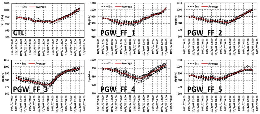
Hydrology 2019, 6, 51                                                                              2 of 15

reduced frequency of TCs globally, with a wide range of predictions among models, ranging from 6
to 34% reduction by the late 21st century. In individual ocean basins, these models project that the
frequency may either increase or decrease by a substantial percentage [1,7,12–21]. However, scientists
have low confidence in projected changes in tropical storm activity in individual ocean basins. There is
some agreement that it is likely that the global frequency of tropical cyclones will either decrease or
remain essentially unchanged in response to 21st-century climate warming [6,10,19,22].
     Tropical storms tend to be larger and more intense in the western North Pacific (WNP) basin than
in any other ocean basin [23]. The typhoons that make landfall on the coasts of Vietnam or Southern
China originate near the Philippines in the South China Sea. Some agencies, such as the Hong Kong
Observatory and the Regional Specialized Meteorological Center in Tokyo, monitor the development,
movement and strength of typhoons in the WNP, and keep historical records of past storms. Every
year, there is an average of five to six typhoons affecting the coastal area of Vietnam. Most of the
typhoons occur from the north to the central region of Vietnam. The typhoon season usually lasts
from June to November, with the highest frequency in September. Sometimes, it may begin as early as
March and last until December.
     When typhoons move in over land, they can cause severe damage, often resulting in human and
economic losses. There are many examples of typhoons leaving an enormous number of casualties
behind. For example, Typhoon Cecil in 1985 caused the deaths of 900 people, and Typhoon Dan in 1989
killed 352 people [24]. Typhoons with strong wind cause severe damage, quickly destroying poorly
constructed houses and other structures. As a result, it is important to predict the variation of typhoon
intensities, in term of minimum sea level pressure (MSLP), maximum wind speed (MWS), and the
spatial distribution of rainfall, as accurately as possible.
     In this study, the pseudo global warming (PGW_FF) downscaling approach [25] was applied.
The primary goal of this paper is to investigate the future change in intensity of typhoons and heavy
rainfall in the coastal area of Vietnam. For this purpose, authors selected Typhoon Lekima in 2007,
and conducted reproductive and pseudo global warming (PGW_FF) experiments to investigate the
intensity changes of the typhoon. Typhoon Lekima was the most destructive storm over this area in
the 2000s, and it caused a heavy loss of human lives and huge damages to properties in Vietnam and
Lao PDR due to storm surge, strong wind, and heavy rainfall.
     In Section 2, an overview of the dataset and design of the dynamic downscaling (DDS) with
PGW forcing data is provided. In Section 3, simulated results of control runs (CTL) and PGW_FF
experiments on Typhoon Lekima are discussed. Finally, a summary is given in Section 4.

2. Data and Methodology

2.1. Data

2.1.1. Japanese 55-Year Reanalysis (JRA-55)
      The Japan Meteorological Agency (JMA) started the second Japanese global atmospheric reanalysis
project, named the Japanese 55-year Reanalysis (JRA-55). It covers 55 years, extending back to 1958
when the global radiosonde observing system was established. Many of the deficiencies found in
the first Japanese reanalysis, the Japanese 25-year Reanalysis (JRA-25), were improved. JRA-55 aims
at providing a comprehensive atmospheric dataset that is suitable for studies of climate change or
multi-decadal variability, by producing a more time-consistent dataset for a longer period than JRA-25.
      The Japanese 55-year reanalysis product (JRA-55) by the Japan Meteorological Agency (JMA)
was used for simulations of the heavy rain event in 2008. JRA-55 was produced by a system based
on the low-resolution (TL319) version of the JMA’s operational data assimilation system, which has
been extensively improved since the previous reanalysis (JRA-25). The atmospheric component of
JRA-55 was based on the incremental four-dimensional variational method. Newly available and
improved past observations are used for JRA-55. Major problems in JRA-25 (cold bias in the lower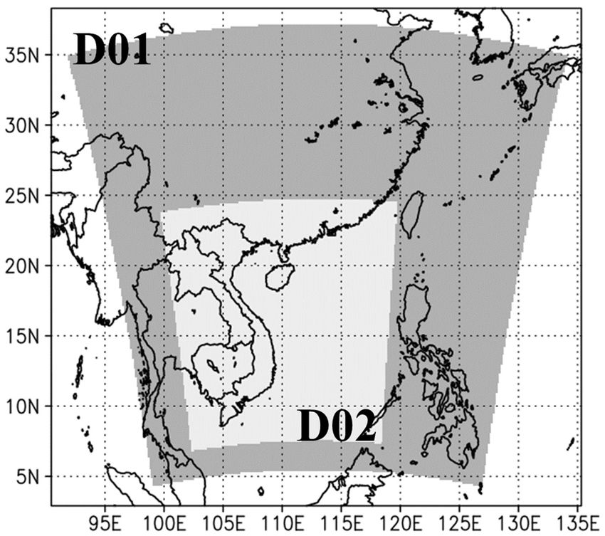
Hydrology 2019, 6, 51                                                                                     3 of 15

stratosphere and dry bias in the Amazon) were resolved in JRA-55; therefore, the temporal consistency
of temperature was improved. Further details are available in Kobayashi et al. [26].

2.1.2. Climate Model Intercomparison Project (CMIP5)
     Global warming experiments, namely, the Climate projections of the fifth phase of the Climate
Model Intercomparison Project (CMIP5), were used for the preparation of the PGW conditions.
In CMIP5 (Taylor et al. 2012) [27], simulations of climate projections were conducted according to
several greenhouse gas emission scenarios, i.e., representative concentration pathways (RCPs). For
example, in the RCP4.5 scenario, the radiative forcing of the Earth becomes 4.5 W/m2 by the end of the
21st century (Taylor et al. 2012) [27]. In this study, projections based on the RCP4.5 scenario were used,
details of which are presented in Table 1.

        Table 1. List of the Climate Model Intercomparison Project (CMIP5) models used in the research.

      CMIP5_ID           Ensemble Name                        Institute                       Country
                                               Canadian Centre for Climate Modelling
       CanESM2              PGW_FF_1                                                          Canada
                                                          and Analysis
                                                  Centre National de Recherches
                                                Meteorologiques/Centre Europeen de
     CNRM_CM5               PGW_FF_2                                                           France
                                                Recherche et Formation Avancees en
                                                        Calcul Scientifique
                                               Met Office Hadley Centre (additional
                                               HadGEM2-ES realizations contributed
    HadGEM2-CC              PGW_FF_3                                                      United Kingdom
                                                by Instituto Nacional de Pesquisas
                                                             Espaciais
                                                    Geophysical Fluid Dynamics
     MIROC-ESM              PGW_FF_4                                                       United States
                                                         Laboratory, USA
                                               Japan Agency for Marine-Earth Science
                                                  and Technology, Atmosphere and
     MRI-CGCM3              PGW_FF_5                Ocean Research Institute (The              Japan
                                                 University of Tokyo), and National
                                                 Institute for Environmental Studies

2.1.3. Sea Surface Temperature (SST)
      The National Oceanic and Atmospheric Administration (NOAA) 14 ◦ daily Optimum Interpolation
Sea Surface Temperature (or daily OISST) is an analysis constructed by combining observations from
different platforms (satellites, ships, buoys) on a regular global grid. A spatially complete SST map is
produced by interpolating to fill in gaps.
      The methodology included a bias adjustment of satellite and ship observations (referenced to
buoys) to compensate for platform differences and sensor biases. This proved critical during the Mt.
Pinatubo eruption in 1991, when the widespread presence of volcanic aerosols resulted in infrared
satellite temperatures that were much cooler than actual ocean temperatures (Reynolds et al. 2007) [28]
      For SST in the simulations, we used the NOAA Optimum Interpolation 1/4 Degree Daily Sea
Surface Temperature Analysis (NOAA OI SST) [28]. The NOAA OI SST dataset has a grid resolution
of 0.25◦ and a temporal resolution of one day. The product uses Advanced Very High-Resolution
Radiometer infrared satellite SST data. Advanced Microwave Scanning Radiometer SST data were
used after June 2002. In situ data from ships and buoys were also used for the large-scale adjustment
of satellite biases.

2.1.4. Land-Surface Conditions
    In this study, we used National Centers for Environmental Prediction (NCEP) data. These NCEP
FNL (Final) Operational Global Analysis data are on 1-degree by 1-degree grids, prepared operationally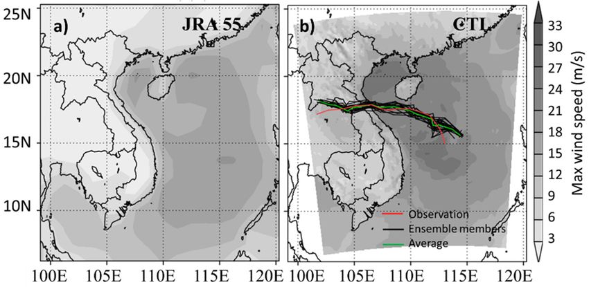
Hydrology 2019, 6, 51 4 of 15
every six hours. This product is from the Global Data Assimilation System (GDAS), which continuously
collects observational data from the Global Telecommunications System (GTS), and other sources,
for many analyses. The FNLs are made with the same model that NCEP uses in the Global Forecast
System (GFS), but the FNLs are prepared about an hour or so after the GFS is initialized. The FNLs are
delayed so that
Hydrology 2019, 6, xmore observational
FOR PEER REVIEW data can be used. The GFS is run earlier in support of time-critical
4 of 15
forecast needs, and uses the FNL from the previous 6-h cycle as part of its initialization. The data
The
spatial analyses is
resolution are
1.0available on the surface,
◦ × 1.0◦ (NCEP at 26 mandatory (and other pressure) levels from 1000
2000) [29].
millibars to 10 millibars, in the surface boundary
The analyses are available on the surface, at layer
26 and at some (and
mandatory sigmaother
layers, the tropopause
pressure) and
levels from
a few others. Parameters include surface pressure, sea level pressure, geopotential
1000 millibars to 10 millibars, in the surface boundary layer and at some sigma layers, the tropopause height,
temperature,
and a few others.sea surface temperature,
Parameters include soil values,
surface ice cover,
pressure, relative
sea level humidity,
pressure, u- and v-winds,
geopotential height,
vertical motion, vorticity, and ozone.
temperature, sea surface temperature, soil values, ice cover, relative humidity, u- and v-winds, vertical
motion, vorticity, and ozone.
2.1.5. Rainfall Data for Verification
2.1.5. Rainfall Data for Verification
As rainfall data for the verification of the Lekima results, we used in situ observation data from
sevenAsrain gauge
rainfall stations
data for theinverification
the coastal regions of Vietnam.
of the Lekima results, Inwe
Vietnam,
used inweather radar stations
situ observation over
data from
the whole
seven rain territory are fairly
gauge stations sparse.
in the Hence,
coastal regionsto examine
of Vietnam. the In detailed
Vietnam,distribution of precipitation
weather radar stations overin
the central region of Vietnam, simulated results were compared with the APHRODITE
whole territory are fairly sparse. Hence, to examine the detailed distribution of precipitation in precipitation
dataset
the (Asian
central Precipitation—Highly-Resolved
region of Vietnam, simulated results Observational
were compared Data
withIntegration towardsprecipitation
the APHRODITE Evaluation).
The APHRODITE
dataset dataset Ver.1101R2, with a spatial
(Asian Precipitation—Highly-Resolved resolutionData
Observational of 0.25° for the Monsoon
Integration towards Asia region,
Evaluation).
was APHRODITE
The used in this study (Yatagai
dataset et al. 2012)
Ver.1101R2, with [30]. ◦
a spatial resolution of 0.25 for the Monsoon Asia region,
was used in this study (Yatagai et al. 2012) [30].
2.1.6. Overview of Tropical Cyclone Lekima
2.1.6. Overview of Tropical Cyclone Lekima
A tropical depression formed in the South China Sea at 06:00 UTC 30 September 2007 at
A tropical 115
approximately depression
oE/14.7 oN.formed in the
Initially, South in
it moved China Sea at 06:00
a northwest UTC towards
direction 30 September
Hainan2007 at
Island
approximately 115 ◦ E/14.7◦ N. Initially, it moved in a northwest direction towards Hainan Island
whilst simultaneously intensifying, before becoming tropical storm named Lekima at 12:00 UTC,
whilst simultaneously
after which it continuedintensifying,
in a northwest before becoming
direction. Then,aittropical storm named
slowly changed Lekima
direction at 12:00 UTC,
to west-northwest
after which it continued
and continued in a northwest
getting stronger. At 00:00direction.
UTC 02Then, it slowly
October, changedinto
it developed direction to west-northwest
a typhoon of category 3
and continued getting stronger. At 00:00 UTC 02 October, it developed into
on the Saffir–Simpson scale, continued its trajectory toward the Vietnamese coast, and hit land a typhoon of category 3 on
at
the Saffir–Simpson
12:00 UTC 03 October scale, continued
at 106.5 o E/17.9itsN.
o trajectory
The mosttoward
dangerous the Vietnamese coast,Lekima
aspects of storm and hitwere
land the
at 12:00
very
UTC
strong03winds, at 106.5◦with
Octobercoupled E/17.9 ◦ N. The most dangerous aspects of storm Lekima were the very strong
heavy rainfall and flooding following its path. Total rainfall exceeded
winds,
400 mm at many observation sites, andflooding
coupled with heavy rainfall and following
the maximum value its was
path.660
Total
mm rainfall
during exceeded 400 mm
24 h in Thua at
Thin
many observation sites, and the maximum value was 660 mm during 24 h in Thua Thin Hue Province.
Hue Province.
The typhoon intensity datasets for calibrations of the Lekima results based on the Japan
Meteorological Agency (JMA) are are shown
shown in in Figure
Figure 1.1.
Figure 1. Minimum sea level pressure (MSLP) and maximum sustained wind speed of Typhoon Lekima
Figure 1. Minimum sea level pressure (MSLP) and maximum sustained wind speed of Typhoon
in 2007.
Lekima in 2007.
2.2. Dynamical Downscaling Method
2.2.1. Pseudo Global Warming Conditions
Control simulations of Lekima (CTL) were performed with initial and boundary conditions
prepared from JRA-55, NCEP FNL and NOAA 0.25 interpolated OI SST. In addition to CTL, we
Hydrology 2019, 6, 51                                                                                           5 of 15

2.2. Dynamical Downscaling Method

2.2.1. Pseudo Global Warming Conditions
     Control simulations of Lekima (CTL) were performed with initial and boundary conditions
prepared from JRA-55, NCEP FNL and NOAA 0.25 interpolated OI SST. In addition to CTL,
Hydrology 2019, 6, x FOR PEER REVIEW                                                                            5 of 15
we performed simulations with PGW forcing, prepared using different CMIP5 data. PGW conditions
of Lekima
were        were from
       obtained      calculated  from future
                           the 10-year         and mean
                                         monthly   presentfrom
                                                            climate
                                                                 2091conditions.
                                                                       to 2100 with ThePGW_FF.
                                                                                         future weather   conditions
                                                                                                    Present  climatic
were  obtained      from   the 10-year   monthly   mean   from   2091  to  2100  with   PGW_FF.
conditions were obtained from the 10-year monthly mean from 1991 to 2000, in historical simulation  Present  climatic
conditions
for CMIP5.wereThen,obtained     from
                        anomalies   of the 10-year
                                        global     monthly
                                               warming   were mean   from 1991
                                                                calculated        to 2000,
                                                                             as the         in historical
                                                                                      difference  added simulation
                                                                                                          to JRA-55.
for CMIP5.     Then,    anomalies   of  global  warming   were   calculated   as  the
Thus, a set of PGW conditions was constructed for the wind, atmospheric temperature,   difference  added  to JRA-55.
                                                                                                        geopotential
Thus,  a set of  PGW     conditions  was   constructed  for the  wind,   atmospheric    temperature,
height, surface pressure and specific humidity. For relative humidity, the original values in JRA-55    geopotential
height,  surfaceinpressure
were retained         the PGWand    specific humidity.
                                conditions,              For
                                              and specific    relative in
                                                           humidity     humidity,    the original
                                                                          these conditions    was values
                                                                                                   definedinfrom
                                                                                                              JRA-55
                                                                                                                   the
were  retained    in  the PGW   conditions,  and  specific humidity    in these  conditions   was
relative humidity and the modified atmospheric temperature of the future climate. To prepare SST   defined  from   the
relative  humidity
for the PGW             and the
                condition,    themodified   atmospheric
                                  SST anomaly    obtainedtemperature
                                                            from future of   the
                                                                           and     futureclimate
                                                                                present    climate.conditions
                                                                                                     To prepare inSST
                                                                                                                   the
for the PGW     condition,    the SST
CIMP5 output was added to the NOAA SST. anomaly  obtained   from  future   and present    climate  conditions   in the
CIMP5 output was added to the NOAA SST.
2.2.2. Design of Numerical Simulations
2.2.2. Design of Numerical Simulations
      In this study, the Weather Research and Forecasting model (WRF) version 3.6.1 was adopted for
      In this study, the Weather Research and Forecasting model (WRF) version 3.6.1 was adopted
the CTL and PGW simulations. A two-way nesting grid system was used, as shown in Figure 2. The
for the CTL and PGW simulations. A two-way nesting grid system was used, as shown in Figure 2.
coarsest domain, D01, had a 30-km horizontal resolution, and the higher resolution domain, D02, had
The coarsest domain, D01, had a 30-km horizontal resolution, and the higher resolution domain, D02,
a 10-km horizontal resolution.
had a 10-km horizontal resolution.

      Figure 2. Target domains of downscaling in the Weather Research and Forecasting (WRF) model.
      Figure 2. Target domains of downscaling in the Weather Research and Forecasting (WRF) model. The
      The spatial resolutions are 30 km and 10 km for D01 and D02, respectively.
      spatial resolutions are 30 km and 10 km for D01 and D02, respectively.

      Ensemble simulations with different initial conditions were performed for the CTL and each PGW
      Ensemble simulations with different initial conditions were performed for the CTL and each
condition. At first, the lagged average forecast (LAF) method (Hoffman and Kalnay 1983) was used to
PGW condition. At first, the lagged average forecast (LAF) method (Hoffman and Kalnay 1983) was
obtain three different conditions: X1 , X2 , and X3 (Figure 3). In LAF, multiple simulations with different
used to obtain three different conditions: X1, X2, and X3 (Figure 3). In LAF, multiple simulations with
initial times were performed. The three simulations were set up with 6-h lags so that the simulations
different initial times were performed. The three simulations were set up with 6-h lags so that the
began at 00:00 UTC, 06:00 UTC and 12:00 UTC on 30 September.
simulations began at 00:00 UTC, 06:00 UTC and 12:00 UTC on 30 September.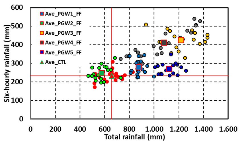
Hydrology 2019, 6, 51                                                                                                6 of 15
  Hydrology 2019, 6, x FOR PEER REVIEW                                                                                6 of 15

     Figure 3. (a) Schematic view of the lagged average forecast (LAF) method, (b) ensemble member
       Figure 3. (a)
     preparation.    Schematic
                   Large        view are
                         open circles of the
                                          the lagged  average
                                              base states       forecast
                                                          (X1 , X 2 , and X(LAF)  method,
                                                                            3 ) made by the (b)
                                                                                            LAFensemble
                                                                                                method. member
                                                                                                        Small
       preparation.
     open circles areLarge
                      newlyopen circles
                            prepared    are the base
                                      ensemble        states (X1, X2, and X3) made by the LAF method. Small
                                                 states.
       open circles are newly prepared ensemble states.
     From three ensemble members, two perturbation states (∆X2 and ∆X3 ) were produced, as follows:
       From three ensemble members, two perturbation states (ΔX2 and ΔX3) were produced, as
  follows:                              ∆X2 = X2 − X1                                           (1)

                                                     Δ3X=
                                                    ∆X  2 =XX
                                                            3−  −1X 1
                                                              2 X                                                        (1)
                                                                                                                        (2)

                                            ΔX = Xequation:
      Then, a new state was made from the following −X     3      3      1                                               (2)

        Then, a new state was made X n =the
                                   from      + α × ∆Xequation:
                                          X1following 2 + β × ∆X3                                                       (3)

      Here, α and β are scale factors ofX∆Xn =
                                             2 and
                                                      α3×. Sixteen
                                                X 1 +∆X              β × Δensemble
                                                            ΔX 2 + new     X3      members were prepared (3)
                                                                                                         at
00:00 UTC on 01 October. In total, 19 simulations were made (Figure 3) until 18:00 UTC 04 October.
        Here, α and β are scale factors of ΔX2 and ΔX3. Sixteen new ensemble members were prepared
Pairs of the scale factors are listed in Table 2. Ensemble simulations enable the stochastic analysis of
  at 00:00 UTC on 01 October. In total, 19 simulations were made (Figure 3) until 18:00 UTC 04 October.
differences between CTL and PGW runs. Therefore, it could be determined whether differences were
  Pairs of the scale factors are listed in Table 2. Ensemble simulations enable the stochastic analysis of
attributable to the effects of global warming or chaotic behaviors in the numerical weather model.
  differences between CTL and PGW runs. Therefore, it could be determined whether differences were
  attributable to the effects of global warming or chaotic behaviors in the numerical weather model.
                                  Table 2. Pairs of the scale factors (α and β).

                        (α, β)          Table (α,
                                              2. Pairs
                                                  β) of the scale factors
                                                                   (α, β) (α and β).        (α, β)

              (α, β) (−1/3, 1/3)                (0, 2/3)
                                               (α,  β)                     (1/3, 2/3)(α, β)        (2/3, 1/3)      (α, β)
                     (−1/3, 2/3)             (1/3, −1/3)                    (1/3, 1)               (2/3, 2/3)
           (–1/3, 1/3)(−1/3, 1)               (0,  2/3)
                                                (1/3, 0)
                                                                                   (1/3, 2/3)
                                                                          (2/3, −1/3)              (1, −1/3)
                                                                                                                 (2/3, 1/3)
           (–1/3, 2/3)(0, 1/3)              (1/3,
                                              (1/3,–1/3)
                                                     1/3)                   (2/3, 0) (1/3, 1)       (1, 1/3)     (2/3, 2/3)
            (–1/3, 1)                         (1/3,  0)                           (2/3,  –1/3)
                                * The original three states (X1 , X2 , and X3 ) are not included.                (1, –1/3)
             (0, 1/3)                        (1/3, 1/3)                              (2/3, 0)                     (1, 1/3)
      Kain–Fritsch cumulus     *Theparameterization
                                      original three states(Kain
                                                              (X1, X  2004),
                                                                        2, and X and   the
                                                                                  3) are notmicrophysics
                                                                                              included.       parameterization
schemes of Lin et al. (1983), were used in this study. Physical processes of the surface layer, land
        Kain–Fritsch cumulus parameterization (Kain 2004), and the microphysics parameterization
surface scheme, and planetary boundary layer scheme were computed by Fifth-Generation Penn
  schemes of Lin et al. (1983), were used in this study. Physical processes of the surface layer, land
State Mesoscale Model (MM5) similarity based on Moni–Obukhov with the Carlson Boland viscous
  surface scheme, and planetary boundary layer scheme were computed by Fifth-Generation Penn
sub-layer, the Noah Land Surface model (Chen et al. 2001), and the Yonsei University scheme (Hong
  State Mesoscale Model (MM5) similarity based on Moni–Obukhov with the Carlson Boland viscous
et al. 2006). For longwave radiation, we used the Rapid Radiative Transfer Model (RRTM) scheme
  sub-layer, the Noah Land Surface model (Chen et al. 2001), and the Yonsei University scheme (Hong
(Mlawer et al. 1997), and for shortwave radiation, we used the Goddard shortwave scheme (Chou and
  et al. 2006). For longwave radiation, we used the Rapid Radiative Transfer Model (RRTM) scheme
Suarez. 1994). For D01, a spectral nudging method was used for atmospheric temperature, zonal wind,
  (Mlawer et al. 1997), and for shortwave radiation, we used the Goddard shortwave scheme (Chou
meridional wind, and geopotential height every six hours at altitudes above 6–7 km. Model settings
  and Suarez. 1994). For D01, a spectral nudging method was used for atmospheric temperature, zonal
are given in Table 3.
  wind, meridional wind, and geopotential height every six hours at altitudes above 6–7 km. Model
  settings are given in Table 3.

                           Table 3. Settings in the Weather Research and Forecasting model.

      Version of Model                                                       V 3.6.1

  Hydrology 2019, 6, x; doi: FOR PEER REVIEW                                              www.mdpi.com/journal/hydrology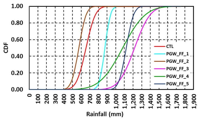
Hydrology 2019, 6, 51                                                                                   7 of 15

                         Table 3. Settings in the Weather Research and Forecasting model.

                Version of Model                                           V 3.6.1
               Number of domain                                             Two
            Horizontal grid distance                     30 km (coarse domain); 10 km (fine domain)
               Cloud microphysics                                     Lin et al. method
           Cumulus parameterization                    Kain–Fritsch scheme cumulus parameterization
               Longwave radiation                      RRTM scheme (Rapid Radiative Transfer Model)
               Shortwave radiation                                   Goddard shortwave
                   Surface layer                                       MM5 similarity
              Land surface scheme                                 Noah Land Surface model
       Planetary boundary layer scheme                            Yonsei University scheme
                                                    A spectral nudging method was used for atmospheric
           Setting of spectral nudging           temperature, zonal wind, meridional wind, and geopotential
                                                      height every six hours, at altitudes above 6–7 km.

3. Results

3.1. Results of the CTL Run
     Results of the CTL run are presented in Section 3.1 to assess typhoon Lekima intensities and,
in comparison with observation data, in terms of MSLP at the center of the simulated typhoon, the
maximum surface wind speed (MWS), the track of Typhoon Lekima, and heavy rainfall.

3.1.1. Minimum Sea Level Pressure, Maximum Wind Speed, and Tracks of the Typhoon

a. Minimum Sea Level Pressure
      Figure 4 illustrates the time evolution of Typhoon Lekima intensity in terms of MSLP. It is clear
that the simulation results of MSLP from nineteen ensemble members show that MSLP is higher than
the estimated value from JMA in the first 60 h of typhoon Lekima, from 06:00 UTC 01 October to 18:00
UTC 03 October. However, after typhoon Lekima made landfall on 12:00 UTC 03 October, the observed
MSLP was higher than the simulated values. For instance, at 18:00 UTC 03 October, observed MSLP
of JMA was 992.5 hPa, compared to 987 hPa average of simulation values from nineteen ensemble
members. The observed values show that the power dissipation of the storm from 980 to 1000 hPa was
faster than the simulated results. The highest difference between a simulated value and an estimated
value was 8 hPa, at 06:00 UTC 02 October. The comparison indicates that all simulations of central
surface pressure agree well with the best-track data, through the intensification of the TC that occurred
before its landfall in Vietnam was slightly delayed.
      Figure 4 shows that from 06:00 UTC 01 October to 12:00 UTC 03 October the spatial correlation
between the simulation results and observation data is stable and comparable. So, it can be used with
the caveat of the direction of the tropical cyclone, for government and people, although the simulation
results are overestimated when compared to observation data.
      From 12:00 UTC 03 October, the time when tropical cyclone Lekima made landfall inland, the
simulation results of MSLP were lower than the observation data, in this case, because the land-surface
conditions used in this study, NCEP_FNL with a resolution of 1◦ × 1◦ , cannot cover the microphysics
of the Truong Son mountain ridge that runs toward the southeast, with the width of the Truong
Son mountain ridge from 30 km to 40 km being much smaller than the minimum considered by the
NCEP_FNL dataset. So, it might not consider the peak of the Truong Son Mountain ridge (the Truong
Son mountain peak is about 2300 m height above sea level), but rather treat it as flat terrain without the
sudden change in topography. So, simulation results of MSLP gradually decreased inland due to a lack
the estimated value from JMA in the first 60 h of typhoon Lekima, from 06:00 UTC 01 October to 18:00
UTC 03 October. However, after typhoon Lekima made landfall on 12:00 UTC 03 October, the
observed MSLP was higher than the simulated values. For instance, at 18:00 UTC 03 October,
observed MSLP of JMA was 992.5 hPa, compared to 987 hPa average of simulation values from
nineteen ensemble members. The observed values show that the power dissipation of the storm from
Hydrology 2019, 6, 51 8 of 15
980 to 1000 hPa was faster than the simulated results. The highest difference between a simulated
Hydrology 2019, 6, x FOR PEER REVIEW 8 of 15
value and an estimated value was 8 hPa, at 06:00 UTC 02 October. The comparison indicates that all
simulations of central
of power, while surface pressure
the observation data ofagree
MSLPwell with the
quickly best-track
decreased data, through
because the intensification
the Truong Son mountain
Figure 4 shows that from 06:00 UTC 01 October to 12:00 UTC 03 October the spatial correlation
of the TCthe
blocked thatstorm,
occurred before
as we its in
can see landfall in Vietnam
12:00 UTC was slightly
03 October to 18:00 delayed.
UTC 04 October (Figure 4).
between the simulation results and observation data is stable and comparable. So, it can be used with
the caveat of the direction of the tropical cyclone, for government and people, although the simulation
results are overestimated when compared to observation data.
From 12:00 UTC 03 October, the time when tropical cyclone Lekima made landfall inland, the
simulation results of MSLP were lower than the observation data, in this case, because the land-
surface conditions used in this study, NCEP_FNL with a resolution of 1o x 1o, cannot cover the
microphysics of the Truong Son mountain ridge that runs toward the southeast, with the width of
the Truong Son mountain ridge from 30 km to 40 km being much smaller than the minimum
considered by the NCEP_FNL dataset. So, it might not consider the peak of the Truong Son Mountain
ridge (the Truong Son mountain peak is about 2300 m height above sea level), but rather treat it as
flat terrain without the sudden change in topography. So, simulation results of MSLP gradually
decreased inland due to a lack of power, while the observation data of MSLP quickly decreased
because the4.Truong
Figure 4.
SonMSLP
mountain
EstimatedMSLP
blocked
fromnineteen
the storm,members
nineteenensemble
as we can
ensemblemembers
seeobserved
in 12:00MSLP
andobserved
UTC 03 October
fromthe
to 18:00
the Japan
Japan
Figure Estimated from and MSLP from
UTCMeteorological
04 October (Figure
Agency4).(JMA).
Meteorological Agency (JMA).
b. Maximum Wind Speed and Tracks
Tracks
Hydrology 2019, 6, x; doi: FOR PEER REVIEW www.mdpi.com/journal/hydrology
Figure 5a,b show the spatial distribution of MWS from JRA-55 data and simulated results of the
model in the period from 06:00 UTC 01 October to 18:00 UTC 04 October.
October. Authors recognize that the
average
average value
value of wind speed from the CTL run tended to be stronger than JRA-55 and expanded from
the north to the south, and from
from the
the sea
sea to
to inland,
inland, during
during the
the typhoon
typhoon in
in Vietnam.
Vietnam.
Figure 5. (a)
Figure 5. (a) Maximum
Maximumwindwindspeed
speed(MWS)
(MWS) from
fromthethe
Japanese 55-year
Japanese Reanalysis
55-year (JRA-55)
Reanalysis dataset
(JRA-55) and
dataset
(b) average MWS and track of typhoon Lekima simulated by WRF models, where the black
and (b) average MWS and track of typhoon Lekima simulated by WRF models, where the black line line and
green line each
and green represent
line each the average
represent tracktrack
the average of nineteen ensemble
of nineteen members,
ensemble and the
members, andred
theline
redisline
the is
track
the
observed by the JMA.
track observed by the JMA.
Figure 5b shows a comparison of predicted and JMA tracks using nineteen ensemble members in
Figure 5b shows a comparison of predicted and JMA tracks using nineteen ensemble members
the D02 domain with 10 km spatial resolution. According to the JMA observations, typhoon Lekima
in the D02 domain with 10 km spatial resolution. According to the JMA observations, typhoon
was formed in the South China Sea at 06:00 UTC 30 September 2007 at approximately 114◦ E/14.7◦ N,
Lekima was formed in the South China Sea at 06:00 UTC 30 September 2007 at approximately 114
and it moved
oE/14.7 in a northwest direction towards Hainan Island. However, the simulation results of
oN, and it moved in a northwest direction towards Hainan Island. However, the simulation
nineteen ensemble members showed that the storm formed near 115◦ E and 15◦ N oand movedo to the
results of nineteen ensemble members showed that the storm formed near 115 E and 15 N and
northwest direction. The simulated tracks passed close to the track observed by the JMA, especially
moved to the northwest direction. The simulated tracks passed close to the track observed by the
the average value from nineteen simulations (green line), not only in terms of the direction but also the
JMA, especially the average value from nineteen simulations (green line), not only in terms of the
location where typhoon Lekima made landfall (at 12:00 UTC 03 October 2007).
direction but also the location where typhoon Lekima made landfall (at 12:00 UTC 03 October 2007).
3.1.2. Rainfall
3.1.2. Rainfall
Figure 6 shows the spatial distribution of total precipitation from the APHRODITE dataset and
Figure 6 shows the spatial distribution of total precipitation from the APHRODITE dataset and
an average of nineteen ensemble members of the CTL run. The results of the CTL run indicate that
an average of nineteen ensemble members of the CTL run. The results of the CTL run indicate that
the spatial distribution of heavy rainfall spread from the north to the south, and was concentrated
Hydrology 2019, 6, x; doi: FOR PEER REVIEW www.mdpi.com/journal/hydrologyHydrology 2019, 6, 51 9 of 15
Hydrology 2019, 6, x FOR PEER REVIEW 9 of 15
the spatial distribution of heavy rainfall spread from the north to the south, and was concentrated
mainly in the central region of Vietnam. The rainfall spatial distribution of the CTL run was similar
to the APHRODITE dataset. However, the quantity of precipitation of the CTL run was higher than
APHRODITE values.
Figure Spatial
Figure 6.6. Spatial distribution
distribution of rain
of heavy heavy rain
from from
01 to 01 to 03
03 October, 2007October,
of Asian2007 of Asian
Precipitation—
Precipitation—Highly-Resolved Observational Data Integration towards Evaluation (APHRODITE)
Highly-Resolved Observational Data Integration towards Evaluation (APHRODITE) data and a
data and a simulation of nineteen ensemble members.
simulation of nineteen ensemble members.
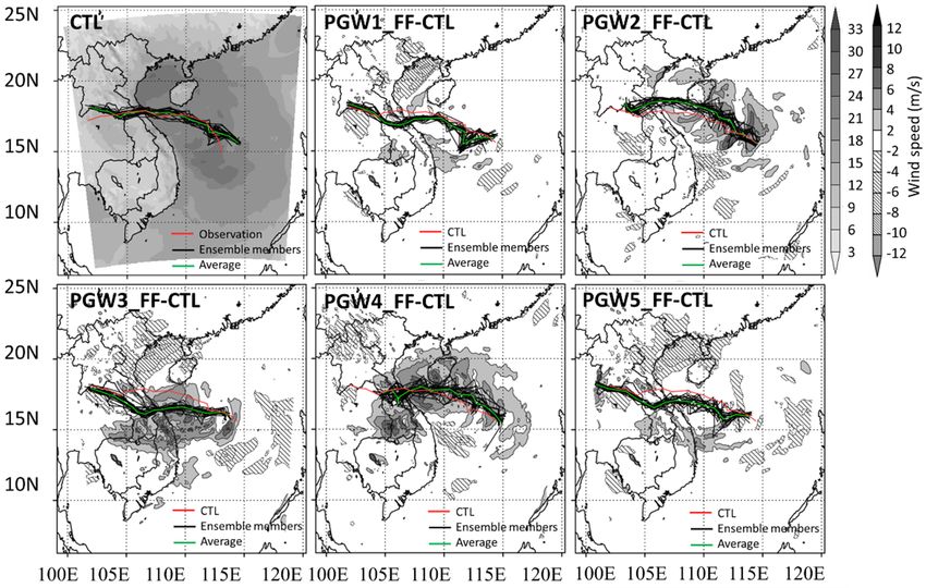
3.2. Results of Pseudo Global Warming Experiments (PGW)
3.2. Results of Pseudo Global Warming Experiments (PGW)
3.2.1. Minimum Sea Level Pressure, Maximum Wind Speed, and Track of Typhoon Lekima
3.2.1. Minimum Sea Level Pressure, Maximum Wind Speed, and Track of Typhoon Lekima
a. Simulated Results of MSLP
a. Simulated Results of MSLP
From Figure 7, the multi-model ensemble experiment results, including the member in each model,
showFrom Figure in
an increase 7, typhoon
the multi-model
intensity.ensemble
At 00:00 UTCexperiment results,
03 October, theincluding
average MSLP the member in each
of 19 ensemble
model, show
members an increase
simulated by theinCTL
typhoon intensity.
run was 983.66At 00:00
hPa, UTC 03 with
compared October, thehPa
972.98 average MSLPhPa
and 979.2 of 19
of
ensemble members
PGW_FF_3 simulated
and PGW_FF_4, by the CTLMeanwhile,
respectively. run was 983.66 hPa, compared
the results of averagewithMSLP 972.98 hPa
of the 19 and 979.2
ensemble
hPa of PGW_FF_3
members simulatedand by PGW_FF_4,
the PGW_FF_1, respectively.
PGW_FF_2, Meanwhile,
and PGW_FF_5the results of average
models are not MSLP
much of the 19
different
ensemble
from members
the results of thesimulated
CTL run.by the PGW_FF
Three PGW_FF_1, PGW_FF_2,
experiments and PGW_FF_5
(PGW_FF_1, PGW_FF_2,modelsandare not much
PGW_FF_5)
different from
simulating thethe results
future of the CTL
produced run.for
results Three PGW_FF
the MSLP experiments
of the typhoon (PGW_FF_1,
that were similarPGW_FF_2,
to thoseandof
PGW_FF_5)
the CTL in the simulating the future
central region producedMeanwhile,
of Vietnam. results for the
twoMSLP
PGW_FF of theexperiments
typhoon that were similar
(PGW_FF_3 andto
those of the CTL
PGW_FF_4) in thethat
predicted central regionwould
the MSLP of Vietnam. Meanwhile,
be lower two PGW_FF
than the results of the CTLexperiments
run. Among (PGW_FF_3
ensemble
and PGW_FF_4)
members in each predicted that the MSLP
PGW_FF experiment, some would be lower
similarities than
were the results
found in MSLP. of These
the CTL run. indicate
results Among
ensemble members in each PGW_FF experiment, some similarities were found in
that the effects of chaotic behaviors are expected to be small, the errors in initial conditions and in model MSLP. These
results indicate
physics result inthat the effects
forecast of chaotic
uncertainties. So,behaviors are expected
global warming mainlytocaused
be small,
the the errors in
difference initial
between
conditions
PGW_FF and in model
experiments andphysics
the CTLresult
run. Inin this
forecast uncertainties.
research, one approachSo, global warming
for reducing thesemainly caused
uncertainties
thethe
is difference between
use of ensemble PGW_FF There
forecasting. experiments
was a wideand variety
the CTL in run. In thisamong
the MSLP research, one approach
the nineteen for
ensemble
reducing these
members in theuncertainties is the use of
PGW_FF experiments andensemble
the CTLforecasting. There was
run. These results a wide variety
demonstrate in the MSLP
the importance of
among thesimulations.
ensemble nineteen ensemble members in the PGW_FF experiments and the CTL run. These results
demonstrate the importance of ensemble simulations.
Hydrology 2019, 6, x; doi: FOR PEER REVIEW www.mdpi.com/journal/hydrologyHydrology 2019, 6, 51 10 of 15
Hydrology 2019,
Hydrology 2019, 6,
6, xx FOR
FOR PEER
PEER REVIEW
REVIEW 10 of
10 of 15
15
Figure The
7. 7.
Figure predicted
The predictedresults
resultsfrom
fromnineteen ensemble
nineteen ensemble membersofofMSLP
ensemble members
members MSLPsimulated
simulated byby control
control (CTL)
(CTL)
Figure 7. The predicted results from nineteen of MSLP simulated by control (CTL)
and
and
PGW_FF
and PGW_FF
PGW_FF
experiments.
experiments.Black
experiments. Blackdash
Black dash lines
dash
and
lines and
lines
thered
and the
the redline
red lineare
line arethe
are theresults
the resultsof
results ofofeach
each
each member
member
member and
and
and
thethe
the
average value
average of
value nineteen
of ensemble
nineteen ensemble members,
members, respectively.
respectively.
average value of nineteen ensemble members, respectively.
b. Max Wind Speed and Tracks
b. Max
b. Max WindWind Speed
Speed andand Tracks
Tracks
The Thesimulation
simulation results
resultsofof
ofthe
thedifference
differencein in MWP
MWP of of Typhoon
of TyphoonLekima Lekimabetween
betweenCTL CTLandand PGW_FF
PGW_FF
The simulation results the difference in MWP Typhoon Lekima between CTL and PGW_FF
experiments
experiments are are shown
are shown
shown inin Figure
in Figure 8.
Figure 8. In
8. In PGW_FF_3
In PGW_FF_3
PGW_FF_3 and and PGW_FF_4
and PGW_FF_4 experiments,
PGW_FF_4 experiments,
experiments, the the
the MWS MWS increased,
MWS increased,
increased,
experiments
strong
strong windwind was
was concentrated
concentrated in
in the
the central
central region
region and
and tended
tended
strong wind was concentrated in the central region and tended to shift to the south over toto shift
shift totothethe south
south over
over time.
time.
time.
Meanwhile,
Meanwhile, the
Meanwhile, the simulation
the simulation results
simulation results of
results of PGW_FF_2
of PGW_FF_2
PGW_FF_2 showedshowed
showed an an increase
an increase
increase in in MWS
in MWS
MWS in in
in the the offshore,
the offshore, before
offshore, before
before
making
making
making landfall.
landfall.PGW_FF_1
landfall. PGW_FF_1and
PGW_FF_1 andPGW_FF_5
and PGW_FF_5 showed
PGW_FF_5 showed
showed aaaslight
slightdecrease
slight decreasein
decrease ininMWS,
MWS,
MWS, compared
compared
compared with
with
with thethe
the
CTLCTL
CTL run.
run.
run.This
Thismay
This maybe
may becaused
be causedby
caused byaaadifference
by difference in
difference in the
in the location
the location of
location of landfall.
of landfall.In
landfall. InInthis
thiscase,
this case,
case, the
thethe maximum
maximum
maximum
wind
wind speed
speedwould
would be affected
be by
affected the
by Truong
the TruongSon mountain
Son mountain ridgeridgethat runs
that
wind speed would be affected by the Truong Son mountain ridge that runs toward the southeast, runstoward
toward the southeast,
the southeast,with
with
thewith
widththe
theof width of the
the Truong
width Truong Son
Son mountain
of the Truong mountain
Son mountain from
fromfrom
30 km 30
30tokm
km to 40
40tokm km
andand
40 km and the
thethepeakpeak
peak about
about
about 2300
2300
2300 m in height.
mmininheight.
height.So,
So,
theSo, the simulation
the simulation
simulation results results
of MWS
results of MWS
of MWS decreased
decreased with
withwith
decreased the typhoon
the typhoon
the typhoon simulated
simulated
simulated by PGW_FF
by PGW_FF
by PGW_FF experiments
experiments
experiments with
with
thewith
same the
the same direction
same
direction direction
of CTLof of CTL run.
CTL
run. run.
Figure
Figure
Figure 8.The
8. 8. Theaverage
The average spatial
average spatial distribution
spatial of MWS
distribution of
distribution of MWS and
MWS andthe
and thetrack
the trackof
track ofofCTL,
CTL,and
CTL, anddifferent
and different
different spatial
spatial
spatial
distributions
distributions of average
distributionsofofaverage
averageMWSMWS between
MWSbetween PGW_FF
between PGW_FF experiments with
experimentswith
PGW_FF experiments tracks
withtracks from
tracksfrom nineteen
fromnineteen
nineteen ensemble
ensemble
ensemble
members
members
members of
ofof
thethe typhoon,and
typhoon,
the typhoon, andthe
and theCTL
the CTLrun.
CTL run.
run.
Hydrology 2019,
Hydrology 2019, 6,
6, x;
x; doi:
doi: FOR
FOR PEER
PEER REVIEW
REVIEW www.mdpi.com/journal/hydrology
www.mdpi.com/journal/hydrologyHydrology 2019, 6, 51 11 of 15
Hydrology 2019, 6, x FOR PEER REVIEW 11 of 15
Figure88shows
Figure showstracks
tracks
in in PGW_FF
PGW_FF models
models withwith nineteen
nineteen ensemble
ensemble members.
members. The simulated
The simulated tracks
tracks
of of PGW_FF_1,
PGW_FF_1, PGW_FF_3, PGW_FF_3, and PGW_FF_5
and PGW_FF_5 experiments
experiments moved to moved to the southern
the southern regions ofregions
Vietnam, of
Vietnam, whereas in the PGW_FF_2 experiment, the typhoon tracks of ensemble
whereas in the PGW_FF_2 experiment, the typhoon tracks of ensemble members seemed to move in members seemed
to move
the in the
direction direction
of the northern of area.
the northern area.track
The average The of
average track showed
PGW_FF_4 of PGW_FF_4 showed
a similar a similar
tendency to the
tendency
CTL to the CTL
run, however, it run, however,
dissipated it quickly.
more dissipated more quickly.
3.2.2.
3.2.2. Simulation Results of Rainfall
a.
a. The
The Magnitude
Magnitude of
of Rainfall
Rainfall
Figure
Figure 99 displays
displays the
the relationship
relationship between
between maximum
maximum six-hourly
six-hourly rainfall
rainfall and
and total
total rainfall
rainfall from
from
00:00
00:00 UTC 01 October to 18:00 UTC 04 October of the CTL run and five PGW_FF models simulating
UTC 01 October to 18:00 UTC 04 October of the CTL run and five PGW_FF models simulating
the future. ItItisisclear
the future. clear that
that bothboth
thethe maximum
maximum six-hourly
six-hourly and and the total
the total simulated
simulated rainfall
rainfall show ashow
stronga
strong increase compared with the simulated rainfall of the CTL run, except for
increase compared with the simulated rainfall of the CTL run, except for the results of the PGW_FF_2 the results of the
PGW_FF_2
experiment,experiment,
where simulatedwhere rainfall
simulated rainfall
slightly slightly decreased
decreased when comparedwhen compared
with the CTL with run.
the CTL
The
run. The highest increase in rainfall was seen in the results of the PGW_FF_3 experiment.
highest increase in rainfall was seen in the results of the PGW_FF_3 experiment. Six-hourly and total Six-hourly
and totalfrom
rainfall rainfall from theensemble
the nineteen nineteen ensemble
members of members
the CTLofrunthewere
CTL232.53
run were
mm232.53 mm and
and 656.38 mm,656.38
rising
mm, risingmm
to 426.46 to 426.46 mm and
and 1217.5 mm1217.5 mm in PGW_FF_3,
in PGW_FF_3, respectively.
respectively. The simulated
The simulated results
results from from
other other
models
models showed an increase from 18% to 76% in both six-hourly and total rainfall,
showed an increase from 18% to 76% in both six-hourly and total rainfall, when compared with the when compared
with
CTL the
run.CTL run.
Figure 9. Simulation results of maximum six-hourly and total rainfall from 00:00 UTC 01 October
Figure 9. Simulation results of maximum six-hourly and total rainfall from 00:00 UTC 01 October to
to 18:00 UTC 04 October of the CTL runs and five PGWs models, in the future simulation in D02.
18:00 UTC 04 October of the CTL runs and five PGWs models, in the future simulation in D02. The x-
The x-axis is total rainfall and the y-axis is maximum six-hourly rainfall. The unit is mm.
axis is total rainfall and the y-axis is maximum six-hourly rainfall. The unit is mm.
In this research, to assess the variation of total rainfall in the future, the authors used cumulative
In this research,
distribution to assess
curves (CDF) andthe variation
assumed theofnormal
total rainfall in the future,
distribution theThe
function. authors used
results arecumulative
shown in
distribution
Figure 10. curves (CDF) and assumed the normal distribution function. The results are shown in
Figure 10.
Figure 10 presents CDF curves of average total rainfall simulated by PGW_FF experiments and
the CTL run. It is clear that there was a significant increase in most of the PGW_FF experiments, except
the CDF curve of PGW_FF_2.
Focusing on the probability of 75%, the results of CTL runs indicated that when a typhoon is
similar to Typhoon Lekima in 2007, with a probability of total rainfall at 75%, the total rainfall from
00:00 UTC 01 October to 18:00 UTC 04 October will exceed 600 mm. On the other hand, the variation
range of average total rainfall is from 720 mm to 1120 mm in most of the PGW_FF experiments.
The maximum increase in rainfall comes from PGW_FF_3 simulations, with 1120 mm. However, the
results of the PGW_FF_2 experiment showed a slight decrease in the total rain, with 410 mm and 530
mm, respectively. The increasing rainfall intensity in the future when simulated by five CMIP5 models
could be explained by the fact that under global warming, water vapor in the atmosphere will be
increased. At the same time, warmer SST will provide more water vapor. These are thought to be the
mainFigure
reasons10.forThe
heavier rainfall
cumulative in the future.
distribution curves of average total rainfall from nineteen ensemble
members simulated by PGW_FF experiments and the CTL run.
Hydrology 2019, 6, x; doi: FOR PEER REVIEW www.mdpi.com/journal/hydrologyFigure 9. Simulation results of maximum six-hourly and total rainfall from 00:00 UTC 01 October to
18:00 UTC 04 October of the CTL runs and five PGWs models, in the future simulation in D02. The x-
axis is total rainfall and the y-axis is maximum six-hourly rainfall. The unit is mm.
In this research, to assess the variation of total rainfall in the future, the authors used cumulative
Hydrology2019,
Hydrology 2019,6,6,51
x FOR PEER REVIEW 12 of 15
12 of 15
distribution curves (CDF) and assumed the normal distribution function. The results are shown in
Figure 10. 10 presents CDF curves of average total rainfall simulated by PGW_FF experiments and
Figure
the CTL run. It is clear that there was a significant increase in most of the PGW_FF experiments,
except the CDF curve of PGW_FF_2.
Focusing on the probability of 75%, the results of CTL runs indicated that when a typhoon is
similar to Typhoon Lekima in 2007, with a probability of total rainfall at 75%, the total rainfall from
00:00 UTC 01 October to 18:00 UTC 04 October will exceed 600 mm. On the other hand, the variation
range of average total rainfall is from 720 mm to 1120 mm in most of the PGW_FF experiments. The
maximum increase in rainfall comes from PGW_FF_3 simulations, with 1120 mm. However, the
results of the PGW_FF_2 experiment showed a slight decrease in the total rain, with 410 mm and 530
mm, respectively. The increasing rainfall intensity in the future when simulated by five CMIP5
models could be explained by the fact that under global warming, water vapor in the atmosphere
will be increased. At the same time, warmer SST will provide more water vapor. These are thought
to beFigure
Figure 10.The
10.
the main Thecumulative
reasons distribution
for heavier
cumulative curves
rainfall
distribution of average
in the
curves future.total rainfall
of average from nineteen
total rainfall ensemble ensemble
from nineteen members
simulated by PGW_FF
members simulated byexperiments and the CTL
PGW_FF experiments andrun.
the CTL run.
b. The Spatial Distribution of Heavy Rainfall
b. The Spatial Distribution of Heavy Rainfall
Hydrology 2019, 6, x; doi: FOR PEER REVIEW www.mdpi.com/journal/hydrology
Figure 11 shows the spatial distribution of total rainfall from 00:00 UTC 01 October to 18:00 UTC
Figure 11 shows the spatial distribution of total rainfall from 00:00 UTC 01 October to 18:00 UTC
04 October of CTL runs and five PGW_FF experiments, in the future simulation in D02. The
04 October of CTL runs and five PGW_FF experiments, in the future simulation in D02. The simulation
simulation results of the PGW_FF_3 and PGW_FF_4 models, when compared with the results of the
results of the PGW_FF_3 and PGW_FF_4 models, when compared with the results of the CTL run,
CTL run, showed heavy rainfall areas covering the region from 14.5 oN to 15.5 oN and 104.5 oE to
showed heavy rainfall areas covering the region from 14.5◦ N to 15.5◦ N and 104.5◦ E to 108.5◦ E.
108.5 oE. The rainfall spatial distribution occurred over a vast area, and it shifted from the north to
The rainfall spatial distribution occurred over a vast area, and it shifted from the north to the south
the south and southwest, extending to Laos and Thailand. This rainfall could cause the severe
and southwest, extending to Laos and Thailand. This rainfall could cause the severe flooding and
flooding and landslides in the central region of Vietnam. Spatial distributions reflect a significant rise
landslides in the central region of Vietnam. Spatial distributions reflect a significant rise in rainfall
in rainfall in the future. However, in the PGW_FF_1 and PGW_FF_5 experiments, heavy rainfall
in the future. However, in the PGW_FF_1 and PGW_FF_5 experiments, heavy rainfall decreased
decreased in the north and showed an increasing trend in the south of the central region, whereas,
in the north and showed an increasing trend in the south of the central region, whereas, the spatial
the spatial distribution of total rainfall as simulated by the PGW_FF_2 experiment showed a
distribution of total rainfall as simulated by the PGW_FF_2 experiment showed a downward trend in
downward trend in heavy rainfall inland, with heavy rainfall concentrated over the South China Sea.
heavy rainfall inland, with heavy rainfall concentrated over the South China Sea. The rain band may
The rain band may be affected by the location of the typhoon where it made landfall. These results
be affected by the location of the typhoon where it made landfall. These results are consistent with
are consistent with previous studies on the effect of climate change on the rainfall distribution caused
previous studies on the effect of climate change on the rainfall distribution caused by the typhoon [31].
by the typhoon [31].
Figure 11. The average total rainfall spatial distribution of nineteen ensemble members of the CTL run,
Figure
and the 11. The average
different total rainfallofspatial
spatial distribution distribution
total rainfall of nineteen
between PGW_FFensemble members
experiments and theofCTL
the run.
CTL
run, and the different spatial distribution of total rainfall between PGW_FF experiments and the CTL
run.
Hydrology 2019, 6, x; doi: FOR PEER REVIEW www.mdpi.com/journal/hydrologyHydrology 2019, 6, 51 13 of 15
In summary, total rainfall in the central regions of Vietnam caused by typhoons similar to Typhoon
Lekima showed a projected increase in intensity in the future. The future spatial distribution of rainfall
tended to shift from north to south and extended to Laos and Thailand. In the future, the results of
rainfall simulated by PGW_FF_3 experiments showed the highest increase in intensity.
4. Conclusions
This study aims to perform a hindcast of typhoon Lekima, which hit the central region of Vietnam
from 30 September to 04 October 2007, and calculates the variations in the intensity of Typhoon Lekima
under global warming climate conditions, applying a downscaling approach to future projection from
five CMIP5 models, using the PGW and ensemble methods.
In the hindcast and in each PGW_FF experiment, nineteen ensemble members were prepared by the
LAF and ensemble methods to examine the differences between simulations caused by global warming.
The simulation results of average MSLP from nineteen ensemble members were overestimated. At the
time when typhoon Lekima made landfall in Vietnam, simulation results were slightly underestimated.
This may be due to the effect of the Truong Son mountain ridge, when compared with the observation
dataset of JMA. The spatial distribution of heavy rainfall caused by Typhoon Lekima shifted from
north to south; however, the location and intensity are different among ensemble members.
In the future simulation with the PGW method, the typhoon intensity and total rainfall tend to
increase when compared with the CTL run. When the typhoon made landfall, the simulated results of
MSLP dropped in most models, and the spatial distribution of the MWS and the typhoon direction
shifted to the southern region. The spatial distribution of total rainfall moved to the southwest to affect
the central areas of Vietnam, Laos, and Thailand. The fluctuation range of rainfall, in six-hourly and
total measurements, was wide among ensemble members of CTL runs and PGW_FF experiments.
An increase in heavy rainfall could occur because, under global warming, saturated vapor will increase
and the warm SST will provide more water vapor and moisture. So, we need to have more mechanisms
of analysis. Furthermore, only one tropical cyclone was examined in this study to draw conclusions
about variations in typhoon intensity due to future global warming, and this may include some degree
of uncertainty.
Our results suggest that under global warming, a tropical cyclone similar to Lekima may bear
more intensity and heavy rainfall in the future. The use of the PGW method and ensemble simulations
can help governments and people living in the coastal region to understand more about the variation
of typhoon intensities, especially the increase in heavy rainfall, which is the main cause of flooding in
Central Vietnam.
Funding: This research received no external funding.
Acknowledgments: Authors are grateful for the use of CMIP5 products archived and published by the Program
for Climate Model Diagnosis and Intercomparison (PCMDI), and to all research institutes contributing to this
activity. Authors would like to thank Vietnam National Hydro-Meteorological Center for providing the observed
rainfall datasets at seven rain gauge stations in the central region. Japanese 55-Year Reanalysis data and the
best-track of Typhoon Lekima were provided by Japan Meteorological Agency. The authors would like to thank
anonymous reviewers for their helpful comments and suggestions to improve the quality of the paper.
Conflicts of Interest: The authors declare no conflict of interest.
References
1. Knutson, T.R.; Tuleya, R.E. Impact of CO2 -induced warming on simulated hurricane intensity and
precipitation: Sensitivity to the choice of climate model and convective parameterization. J. Clim. 2004, 17,
3477–3495. [CrossRef]
2. McDonald, E.R.; Bleaken, D.G.; Cresswell, D.R.; Pope, V.D.; Senior, C.A. Tropical storms: Representation and
diagnosis in climate models and the impacts of climate change. Clim. Dyn. 2005, 25, 19–36. [CrossRef]
3. Chauvin, F.; Royer, J.F.; Deque, M. Response of hurricane-type vortices to global warming as simulated by
arpege-climat at high resolution. Clim. Dyn. 2006, 27, 377–399. [CrossRef]You can also read