A Comparative Study between Regression and Neural Networks for Modeling Al6082-T6 Alloy Drilling - MDPI
←
→
Page content transcription
If your browser does not render page correctly, please read the page content below
machines
Article
A Comparative Study between Regression and Neural
Networks for Modeling Al6082-T6 Alloy Drilling
Nikolaos E. Karkalos 1 , Nikolaos Efkolidis 2 , Panagiotis Kyratsis 2, *      and
Angelos P. Markopoulos 1
 1   School of Mechanical Engineering, Section of Manufacturing Technology, National Technical University of
     Athens, Heroon Polytechniou 9, 15780 Athens, Greece; nkark@mail.ntua.gr (N.E.K.);
     amark@mail.ntua.gr (A.P.M.)
 2   Department of Mechanical Engineering & Industrial Design, Western Macedonia University of Applied
     Sciences, GR 50100 Kila Kozani, Greece; efknikos@gmail.com
 *   Correspondence: pkyratsis@teiwm.gr; Tel.: +30-24610-68086

 Received: 31 December 2018; Accepted: 29 January 2019; Published: 2 February 2019

 Abstract: Apart from experimental research, the development of accurate and efficient models
 is considerably important in the field of manufacturing processes. Initially, regression models
 were significantly popular for this purpose, but later, the soft computing models were proven
 as a viable alternative to the established models. However, the effectiveness of soft computing
 models can be often dependent on the size of the experimental dataset, and it can be lower
 compared to that of the regression models for a small-sized dataset. In the present study, it is
 intended to conduct a comparison of the performance of various neural network models, such as the
 Multi-layer Perceptron (MLP), the Radial Basis Function Neural Network (RBF-NN), and the Adaptive
 Neuro-Fuzzy Inference System (ANFIS) models with the performance of a multiple regression model.
 For the development of the models, data from drilling experiments on an Al6082-T6 workpiece for
 various process conditions are employed, and the performance of models related to thrust force (Fz )
 and cutting torque (Mz ) is assessed based on several criteria. From the analysis, it was found that the
 MLP models were superior to the other neural networks model and the regression model, as they
 were able to achieve a relatively lower prediction error for both models of Fz and Mz .

 Keywords: drilling; Al6082-T6; multiple regression; multi-layer perceptron; radial basis function
 neural network; adaptive neuro-fuzzy inference system; thrust force; cutting torque

1. Introduction
     Aluminum is among the most widely-used metallic elements. Due to its beneficial properties
such as being lightweight and having high corrosion resistance for a considerable range of factors, it is
preferred for the fabrication of various parts in the automotive and aerospace industry. Aluminum is
often found in the form of an alloy with various elements such as copper, magnesium, manganese,
and silicon, among others, and can be subjected to special treatment such as quenching or precipitation
hardening in order to alter its properties, such as strength. Various aluminum alloys exhibit
considerably high strength-to-weight ratios, and most of the alloys have excellent machinability.
     As aluminum is used for a wide variety of applications, a large amount of experimental work has
already been conducted regarding various machining processes. Especially in the case of the drilling
process, several parameters regarding the influence of process parameters on the forces, surface quality,
or tool wear have been conducted, providing useful details for the appropriate processing of this
material. Nouari et al. [1] investigated the effect of drilling process parameters and tool coating on
tool wear during dry drilling of AA2024 aluminum alloy. They noted that at a certain cutting speed,

Machines 2019, 7, 13; doi:10.3390/machines7010013                            www.mdpi.com/journal/machines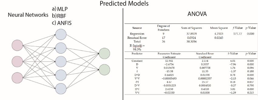
Machines 2019, 7, 13                                                                               2 of 18

a transition in tool wear mechanisms occurs, leading in higher tool wear, and thus, they investigated the
shift in wear mechanism for various tool coating materials. Their results indicated that, at high cutting
speeds, larger deviations from the nominal hole diameters are obtained mainly due to the higher
temperature generated on the rake face of the tool, leading to increased tool damage. While abrasion or
adhesion wear is observed for lower speeds in the form of built-up edge or built-up layer, the increase
of temperature for high cutting speeds resulted in diffusion wear and the increase of the material
adhered to the tool. Furthermore, although the uncoated tool produced more accurate hole dimensions
at low cutting speeds, this trend was reversed in the case of higher cutting speeds, and the use of
the uncoated HSS tool was found to produce the least accurate holes. Girot et al. [2] also conducted
experiments regarding tool wear during dry drilling of aluminum alloys. In their work, they aimed
at the reduction of the built-up layer in the cutting tool by altering the process parameters and tool
coating and geometry. They employed an uncoated carbide drill, a nano-crystalline diamond-coated
drill, a nano-crystalline Balinit-coated drill, and a Mo diamond-coated drill and conducted experiments
with variable cutting speed. After they established the relationship between the cutting parameters,
thrust force, and burr height, they found that diamond coatings were superior due to their low friction
coefficient and adequate adhesion of the coating on the tool, and the nano-structured diamond coated
tools were the best performing in particular.
      Farid et al. [3] conducted a study on chip morphology during high speed drilling of Al-Si alloy.
More specifically, they investigated the effect of cutting speed and feed rate on chip morphology by
conducting observations at various surfaces of the chip using microscopy techniques. For the drilling
experiments, uncoated WC drills were employed to produce 15 mm-diameter holes under various
cutting speeds and feed values, in the range of 240–320 m/min and 0.16–0.24 mm/rev, respectively.
It was found that, on the free surface of the chip, lamella structures were created and that an increase
of speed and feed rate led to a decrease of the frequency of the appearance of these lamella structures.
Regarding chip morphology, the increase of cutting speed and feed led to the increase of chip pitch
and height and a decrease of the chip compression ratio. Finally, thrust force was found to increase
with a decrease of cutting speed and an increase of the feed rate, so it was suggested that high cutting
speeds are essential in order to minimize thrust force in the case of Al-Si alloys’ drilling.
      Qiu et al. [4] investigated the use of high-performance drills during drilling of aluminum and
titanium alloys with a view toward minimizing cutting force and torque. For their experiments,
they employed two conventional and two modified types of drills, which had larger point, primary
relief, and helix angles and a lower second clearance angle. For the aluminum alloy, the cutting speed
was varied from 100–200 m/min and the feed rate from 0.1–0.2 mm/rev. The experiments indicated
that the tools with the modified geometry were able to reduce thrust force and torque in the majority
of cases, with the average reduction of force being 9.78% and torque 21.08%. Dasch et al. [5] conducted
a thorough comparison regarding various categories of coated cutting tools for the drilling process
of aluminum. For their study, they used five different types of coating materials, namely carbon,
graphitic, hydrogenated and hydrogen-free diamond-like carbon, and diamond on two types of drills,
namely HSS and carbide drills. In the tests, they measured tool wear, temperature, and spindle power.
After conducting tests on various cases of cutting speed and feed combinations, they concluded that
the most important is to coat the flutes of the tool rather than the cutting edge, that coated tools were
able to drill up to 100-times more holes than the uncoated, and that hydrogenated carbon coatings are
superior to the other types of coating.
      Regarding modeling of the drilling process, various studies have been conducted due to its
popularity. Kurt, Bagci, and Kaynak [6] determined the optimum cutting parameters for high surface
quality and hole accuracy using the Taguchi method. In their work, they conducted experiments at
various cutting speeds, feed rates, and depths of drilling and tested the performance of both uncoated
and coated HSS drills. After the experiments were conducted by the Taguchi method, regression
models for Ra, and hole diameter accuracy were derived, and the optimum parameters were identified
by analyzing the S/N ratio results. Kilickap [7] used the Taguchi method and Response Surface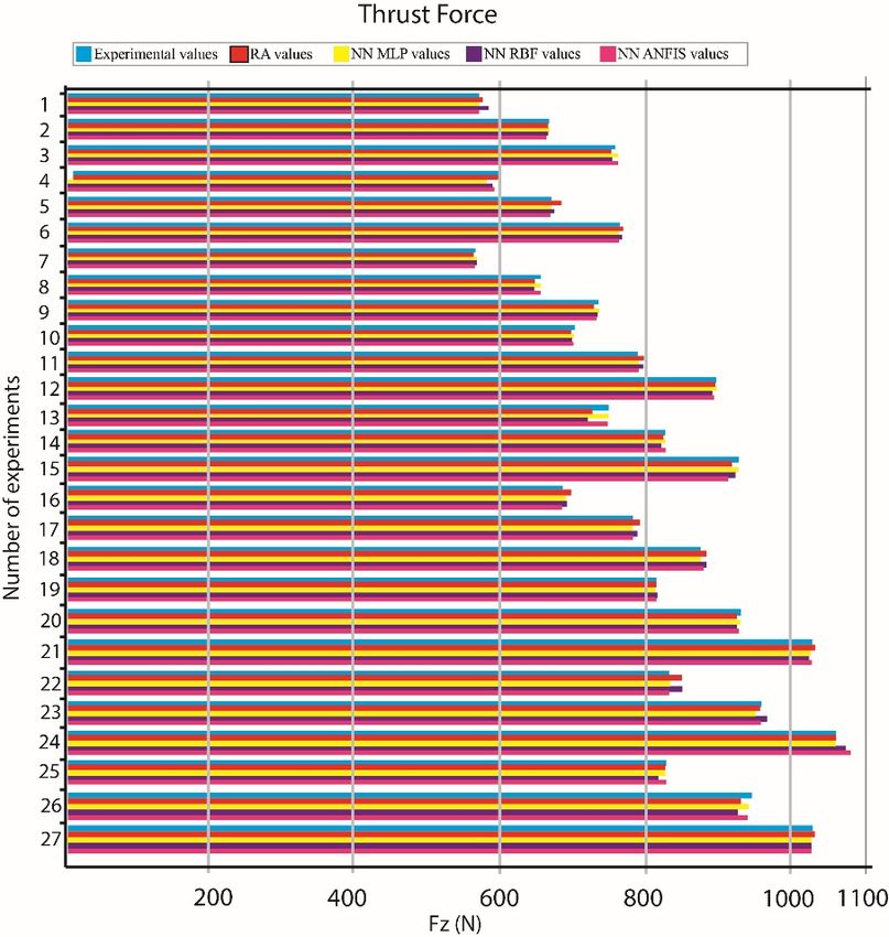
Machines 2019, 7, 13                                                                              3 of 18

Methodology (RSM) to predict burr height during drilling of aluminum alloys and to determine the
optimum drilling parameters. He conducted experiments using various cutting speeds, feed rates,
and point angles and observed the burr height and surface roughness. Analysis using the Taguchi
method and Analysis Of Variance (ANOVA) revealed the optimum parameters for reducing the burr
height and surface roughness, and regression models created using RSM were proven to be adequate
to describe the correlation between process parameters and process outcome. Sreenivasulu and Rao [8],
Efkolidis et al [9], and Kyratsis et al [10] also employed the Taguchi method to determine the optimum
levels of the process parameters for the minimization of thrust force and torque during drilling of
aluminum alloys. After they performed experiments at various cutting speeds, feed rates, and various
drill diameters and geometries, they determined the most significant parameters of the process and
their optimum values.
      Apart from regression models, several studies based on neural network models have been
reported in the relevant literature. Singh et al. [11] employed an Artificial Neural Network (ANN)
model to predict tool wear during drilling of copper workpieces. As inputs for the neural network,
feed rate, spindle speed, and drill diameter were selected, and thrust force, torque, and maximum wear
were the outputs. After the optimum number of hidden layers and neurons, as well as the optimum
learning rate and momentum coefficient were determined, it was shown that the best neural network
predicted tool wear with a maximum error of 7.5%. Umesh Gowda et al. [12] presented an ANN model
for the prediction of circularity, cylindricity, and surface roughness when drilling aluminum-based
composites. After the experiments, tool wear, surface roughness, circularity, and cylindricity were
obtained as a function of machining time, and NN models were used to correlate process parameters
with these quantities.
      Besides the usual MLP models, other similar approaches such as RBF-NN or hybrid approaches
combining MLP with fuzzy logic or genetic algorithms have also been presented. Neto et al. [13] also
presented MLP and ANFIS models for the prediction of hole diameter during drilling of various
alloys. For the neural network models, inputs from various sensors such as acoustic emission,
electric power, force, and vibration were employed. Thorough analysis of the predicted results’
errors revealed that MLP models had superior performance to ANFIS models. Ferreiro et al. [14]
conducted a comprehensive study in developing an AI-based burr detection system for the drilling
process of Al7075-T6. For that reason, they employed data-mining techniques and tested various
approaches with a view toward reducing the classification errors. All developed models performed
better than the existing mathematical model for burr prediction, and in particular, it was shown that
a model based on the naive Bayes method exhibited the maximum accuracy.
      Lo [15] employed an ANFIS model for the prediction of surface roughness in end milling. In their
models, they employed both a triangular and trapezoidal membership function with 48 sets of data
for training and 24 for testing. The error was found to be minimum using the triangular membership
function. Zuperl et al. [16] used an ANFIS model for the estimation of flank wear during milling.
The model was trained with 140 sets of data (75 for training and 65 for testing) and included 32
fuzzy rules. It was shown that a model with a triangular membership function was again capable
of exhibiting the lowest error. Song and Baseri [17] applied the ANFIS model for the selection of
drilling parameters in order to reduce burr size and improve surface quality. In this work, a different
model was built for each of the four outputs, namely burr height, thickness, type, and hole overcut.
One hundred and fifty datasets were used, 92 for the training, 25 for checking, and 25 for testing of
the model. For the first output, the best model had four membership functions of a triangular type;
for the second one, the best model had a three-membership function of a Gaussian type; and the last
two three- and four-membership functions of a generalized bell type, respectively. Fang et al. [18] used
an RBF model for surface roughness during machining of aluminum alloys. Their model included
eight inputs, related to process parameters, cutting forces, and vibration components, and five outputs,
related to surface roughness. The RBF model was proven to be faster than an MLP model, but it was
inferior in terms of accuracy. Elmounayri et al. [19] employed an RBF model for the prediction of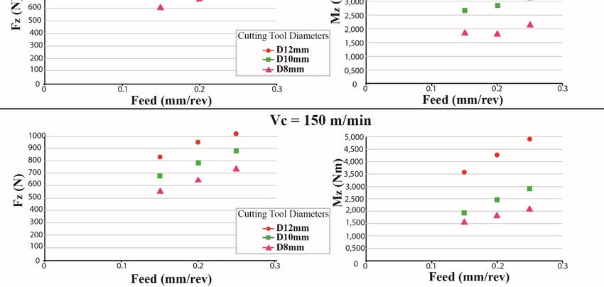
Machines 2019, 7, 13                                                                                 4 of 18

cutting forces during ball-end milling. The model had four inputs, related to the process parameters
and four outputs, namely the maximum, minimum, mean, and standard deviation of instantaneous
cutting force. In this case, it was noted that the RBF network was more efficient and accurate and faster
than the classical MLP.
     Although comparisons between regression models and neural network model for cases of
machining processes have already been conducted, comparison between several soft computing
methods has rarely been conducted, and only a few relevant studies exist. Tsai and Wang [20]
conducted a thorough comparison between various neural network models such as different variants
of MLP, RBF-NN, and ANFIS for the cases of electrical discharge machining. They concluded that
the best performing method was ANFIS, as it exhibited the best accuracy among the tested methods.
Nalbant et al. [21] conducted a comparison between regression and artificial neural network models
for CNC turning cases and concluded that although the neural network model was performing slightly
better, both models were appropriate for modeling the experimental results. Jurkovic et al. [22]
compared support vector regression, polynomial regression, and artificial neural networks in the
case of high-speed turning. Their models included feed, cutting speed, and depth of cut as inputs,
and separate models were created for three output quantities, namely cutting forces, surface roughness,
and cutting tool life. In the cases of cutting force and surface roughness, they found that the polynomial
regression model was the best, whereas in the case of cutting tool life, ANN performed better than the
other methods.
     In the present study, a comparison of various neural network models, as well as multiple
regression models is conducted with a view toward determining the best performing model for
the case of drilling Al6082-T6. As in this case, a relatively small dataset is used, it is expected that the
results of regression models and neural network models will be comparable, and so, it is interesting to
find out whether there can be a clear difference in the performance of these methods in the present case.
The various neural network models are trained with different parameters, and the comparison between
them is conducted by criteria relevant to the prediction error, both for training and testing datasets.

2. Artificial Neural Networks
     Artificial neural networks are among the most important soft computing methods, widely used
for a great range of applications spanning across various scientific fields. This method is able to
successfully predict the outcome of a process by using pairs of input and output data in a learning
procedure. In fact, this method imitates the function of biological neurons, which receive inputs, process
them, and generate a suitable output. The most common ANN model, namely MLP, has a structure
containing various interconnected layers of neurons, starting from an input layer and ending at
an output layer. The middle layers are called hidden layers, and their number is variable, depending
on the size and the characteristics of each problem. Each neuron is connected by artificial synapses to
the neurons of the following layer, and a weighting coefficient, or weight, is assigned to each synapse.
The inputs for each neuron are multiplied by the weighting coefficient of the respective synapse,
and then, they are summed; after that, the output from each neuron is generated by using an activation
function, which usually is a sigmoid function, such as the hyperbolic tangent.
     The ANN model is created by a learning process, containing three different stages, i.e., training,
validation, and testing. For each stage, a part of the total input/output data is reserved, most commonly
70%, 15%, and 15%, respectively. The learning process consists of the determination of suitable weight
values according to real input/output data pairs and is an iterative process. This process is called error
backpropagation, as the difference of the predicted and actual output is first computed in the output
layer, and then, the error is propagated through the network in the opposite way, from the output to the
input layer; after various iterations, or epochs, the network weights are properly adjusted so that the
error is minimized. The training and validation stage both involve adjustment of the weights, and it is
possible to stop the learning process if the error is not decreasing after some epochs, a technique that is
named the early stopping technique. Finally, during the testing stage, the trained model is checked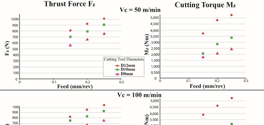
Machines 2019, 7, 13                                                                                 5 of 18

for its generalization capabilities by providing it with unknown data from the testing data sample.
Usually, the Mean Squared Error (MSE) is used for the determination of model performance:

                                                  1 n
                                                  n i∑
                                         MSE =          (Yi − Ai )2                                     (1)
                                                     =1

where n is the number of data samples, Yi are the predicted values and Ai the actual values.
     Furthermore, the Mean Absolute Percentage Error (MAPE) can be also employed to evaluate the
results of neural network models:

                                                 100% n Yi − Ai
                                                   n i∑
                                      MAPE =                                                            (2)
                                                      =1
                                                           Ai

     Finally, RBF-NN is constructed by using an appropriate radial function as the activation function
for a neural network model with a single layer. Most commonly, a Gaussian-type function is used as
the activation function:
                                                         2
                                            ϕ(r ) = e−εr                                            (3)

where ε is a small number and r = k x − xi k, with x being an input and xi the center of the radial basis
function. Apart from the widely-used MLP model and RBF-NN models, various other types of neural
networks exist, as well as hybrid models, combining ANN with other soft computing methods such
as fuzzy logic. In addition to the learning and optimization ability of the neural networks, fuzzy
logic systems are able to provide a means for reasoning to the system with the use of IF-THEN rules.
ANFIS is a soft computing method with characteristics related both to neural networks and fuzzy
logic. Generally, the creation of an ANFIS model has several similarities to the creation of a MLP
model, but there exist also some basic differences. This model has a structure similar to the MLP
structure, but there are some additional layers, related to membership functions of the Fuzzy Inference
System (FIS). One of the most common fuzzy models used in ANFIS models is the Sugeno fuzzy
model. By the training process, fuzzy rules are formed, and an FIS is created. At first, the input
data are converted into fuzzy sets through a fuzzification layer, and then, membership functions are
generated. Membership functions can have various shapes such as triangular, trapezoid, or Gaussian,
among others. In the second layer, the number of nodes is equal to the number of fuzzy rules of
the system; the determination of the number of fuzzy rules is conducted using a suitable method
such as the subtractive clustering method. The output of the second layer nodes is the product of
the input signals, which they receive from the previous nodes. Then, in the third layer, the ratio of
each rule’s firing strength to the sum of the firing strengths of all rules is calculated, and it is used in
the defuzzification layer to determine the output values from each node. Finally, the total output is
calculated by summation of the outputs of the fourth layer. The FIS parameters are updated by means
of a learning algorithm in order to reduce the prediction error, such as in the case of MLP model.

3. Methods and Materials

3.1. Technics of Experiments
    In the present work, it is intended to conduct a comparison of various methods, which can be
employed for modeling of the drilling process of Al6082-T6. The datasets for the models were obtained
by conducting experiments on an Al6082-T6 workpiece. This work material used for the present
investigation was a 140 mm × 100 mm × 30 mm plate with the chemical composition and main
mechanical properties as summarized in Table 1.
Machines 2019, 7, x FOR PEER REVIEW 6 of 19
Machines 2019, 7, 13 Table 1. Chemical composition and mechanical properties of Al6082. 6 of 18
Chemical Composition
Elements Mg Cu
Table 1. Chemical Cr
composition andFe Si Mn of Al6082.
mechanical properties Others Al
Percentage 0.8 0.1 0.25 0.5 0.9 0.5 0.3 Balance
Chemical Composition
Mechanical Properties
Elements Mg Cu Cr Fe Si Mn Others Al
Percentage 0.8 0.1 0.25 Coefficient
0.5 of 0.9 0.5 0.3 Balance
Thermal Melting Elastic Electrical
Alloy Temper Thermal
Conductivity Mechanical Properties Point Modulus Resistivity
Thermal Expansion
Coefficient of Thermal Melting Elastic Electrical
Alloy Temper
Conductivity Expansion Min
Point Modulus Resistivity
W/m·K K−1 GPa Ω·m
Max
Min
W/m·K K−1 GPa Ω ·m
Max
555
Al6082
Al6082 T6
T6 180
180 24
24 × 10
×
− 610 −6 555 70
70
0.038 × 10⁻⁶
0.038 × 10⁻⁶
650
650
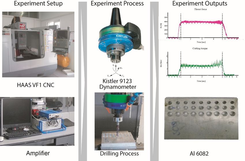
Drilling
Drillingexperiments
experiments were carried
were out out
carried on a on
HAAS VF1 CNC
a HAAS VF1 machining center using
CNC machining solid
center carbide
using solid
drill tools. Two components of drilling loads (thrust force
carbide drill tools. Two components of drilling loads (thrust F z and torque M values) were recorded
force Fz andz torque Mz values) were
with a Kistler
recorded withdynamometer Type 9123Type
a Kistler dynamometer connected to a three-channel
9123 connected charge amplifier
to a three-channel with a data
charge amplifier with
acquisition system. Dynoware software (Type 2825D-02) was used in order to monitor
a data acquisition system. Dynoware software (Type 2825D-02) was used in order to monitor and record the
and
experimental values of thevalues
record the experimental cutting
offorces, as shown
the cutting in as
forces, Figure
shown 1. in Figure 1.
Figure1.1.The
Figure Theworkflow
workflowused
usedfor
forthe
theresearch.
research.
3.2.
3.2.Methodology
MethodologyofofResults
ResultsAnalysis
Analysis
The
Theexperiments
experiments were conducted
were according
conducted to a full
according tofactorial
a full strategy.
factorial The three cutting
strategy. parameters
The three cutting
selected for the
parameters present
selected forinvestigation were the cutting
the present investigation werespeed (V), thespeed
the cutting feed rate
(V), (f),
theand
feedthe cutting
rate (f), andtool
the
diameter (D).diameter
cutting tool Cutting velocity values
(D). Cutting of 50 m/min,
velocity values of100
50m/min,
m/min, and 150 m/min
100 m/min, and together
150 m/min with feed
together
rates
withof 0.15rates
feed mm/rev,
of 0.150.2 mm/rev,
mm/rev, 0.2and 0.25 mm/rev
mm/rev, and 0.25were used
mm/rev in combination
were with three
used in combination cutting
with three
tool diameters
cutting (D) of 8 mm,
tool diameters 108mm,
(D) of andmm,
mm,10 12 mm.
and The constant
12 mm. depth of depth
The constant the holes drilled
of the holeswas 30 mm.
drilled was
The machining parameters used and their levels are shown in Table
30 mm. The machining parameters used and their levels are shown in Table 2. 2.
Machines 2019, 7, x FOR PEER REVIEW 7 of 19
Machines 2019, 7, 13 7 of 18
Machines 2019, 7, x FOR PEER REVIEW 7 of 19
Table 2. Machining factors and their levels.
Table2.2.Machining
Factors
Table Machining factors and
Notation
factors and their
theirlevels.
Levels
levels.
Factors Notation I II
Levels III
Factors Notation Levels
Cutting speed (m/min) V 50I 100 II 150 III
I II III
Feed rate
Cutting (mm/rev)
speed (m/min) f V 0.15 50 0.2
100 0.25
150
Cutting speed (m/min) V 50 100 150
Tool
Feed diameters
Feed
raterate (mm)
(mm/rev)
(mm/rev) D
f f 0.158
0.15 10
0.2 12 0.25
0.2 0.25
Tool
Tool diameters
diameters (mm) (mm) DD 8 8 10
10 12 12
During the experimental process, 27 different solid carbide drilling tools (one tool for each hole)
were clamped
During
During tothe
the aexperimental
Weldon clamping
experimental process,device
process, 27 with a high
27 different
different solid rigidity,
solid carbide while atools
carbidedrilling
drilling mechanical
tools(one
(onetool vise was
forfor
tool each
each used
hole)
hole)
for were clamped
clamping the to a Weldon clamping
workpiece. As the device
type ofwith a high
cutting rigidity,
tools while a mechanical
(KENNAMETAL vise was usedis
B041A/KC7325)
were clamped to a Weldon clamping device with a high rigidity, while a mechanical vise was used for
for clamping the solid
non-through workpiece. As thecutting
type offluid
cutting
usedtools (KENNAMETAL
2270) wasB041A/KC7325) is
clamping thecoolant
workpiece. As carbide,
the typetheof cutting tools (KOOLRite
(KENNAMETAL B041A/KC7325) provided by the
is non-through
non-through
delivery coolant solid carbide, the cutting fluid used (KOOLRite 2270) was provided by the
coolantsystem near them.
solid carbide, Figure fluid
the cutting 2 demonstrates
used (KOOLRiteall the 2270)
dimensional details by
was provided of the
the main
deliveryshape of
system
the deliverytools.
cutting system All near
the them. Figure
possible 2 demonstrates
combinations of the all the dimensional
manufacturing details ofwere
parameters the main
used shape of
(cutting
near them. Figure 2 demonstrates all the dimensional details of the main shape of the cutting tools.
thefeed
speed, cutting
rate,tools.
tool All the possible combinations of the manufacturing parameters were used (cutting
diameter).
Allspeed,
the possible combinations
feed rate, tool diameter).
of the manufacturing parameters were used (cutting speed, feed rate,
tool diameter).
Figure 2. Cutting
Figure tool
2. Cutting geometry
tool geometrydetails.
details.
Figure 2. Cutting tool geometry details.
As shown in Figure 3, apart from multiple regression
regressionmethod, three soft computing methods,
methods,
AsAs shown
shown ininFigure
Figure3,3,apart
apart from
from multiple
multiple regression method,
method,three
threesoft
softcomputing
computing methods,
related to
relatedartificial neural networks, namely MLP, RBF-NN, and ANFIS methods, were used.
related to to artificial
artificial neuralnetworks,
neural networks,namely
namelyMLP,
MLP,RBF-NN,
RBF-NN, and
and ANFIS
ANFIS methods,
methods, wereused.
used.
Figure 3. Development of the predicted models.
Figure 3. 3.
Figure Development ofof
Development the predicted
the predictedmodels.
models.
For the development of the model, MATLABTM software was employed. For each method, only
For the development of related
the model, TM software
theMATLAB
TM software was employed. For each method, only
oneFor the development
characteristic, mainly of the model,
to MATLAB
architecture of the network, was
wasemployed.
varied, and Forother
the eachsettings
method,
one characteristic,
only
wereoneassumed mainly
characteristic, related
mainly
to be equal to to
thethe
related architecture
to the
default ofofthe
architecture
settings network,
the was Forvaried,
of the network,
software. thewasand
MLP the other
varied,
and and settings
RBF-NN,the the
other
were assumed
number of to be
hidden equal
neurons to the
was default
varied, settings
and for of
the the
ANFIS, software.
where For
the the
number
settings were assumed to be equal to the default settings of the software. For the MLP and RBF-NN, MLP
of and
inner RBF-NN,
nodes cannotthe
number
thebe of hidden
altered
number of theneurons
inhiddensame way
neuronswas varied,
aswas
in the andand
other
varied, for the
two ANFIS,
types
for the of where
networks,
ANFIS, thethe
where number
number
number ofclusters
of inner
of nodes
innerused
nodescannot
for the
cannot
bebe data,
altered using
alteredininthe the
same
the fuzzy
same wayc-means
way asasinin clustering
thetheother
other method,
twotwo types
typeswhich
ofof directly the
networks,
networks, affects
the the number
number
number ofof of parameters
clusters
clustersused
used for ofthe
the
for
data,the system,
using the was
fuzzy varied.
c-meansIn all cases,
clustering the lower
method, and upper
which boundaries
directly for
affects
data, using the fuzzy c-means clustering method, which directly affects the number of parameters the
the variable
number parameters
of parameterswere ofof
the
thechosen
system,
system, in
was a
was way
varied.that
varied.InInit did
allall not
cases,
cases, lead
the lower
the to
lower extreme
andandupperoverfitting;
upper the
boundaries
boundaries analysis
forfor
the conducted
variable
the variable was
parameters able
parameters to
were
were
chosen
chosenininaa way that thatititdid
didnotnotleadlead to extreme
to extreme overfitting;
overfitting; the analysis
the analysis conductedconducted
was ablewas able to
to determine
exactly the limit values of the variable parameters, which can lead to a properly-functioning model.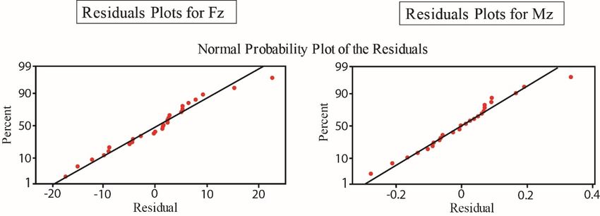
Machines 2019, 7, 13 8 of 18
Machines 2019, 7, x FOR PEER REVIEW 8 of 19
determine
The choice exactly
of thethe limitofvalues
number hidden of the variable
neurons is crucial parameters,
in the case ofwhichMLP and can RBF-NN,
lead to asa it
properly-functioning model.
can increase the accuracy of the network up to a point, and then, it causes problems of overfitting.
The choice of the number of hidden neurons is crucial in the case of MLP and RBF-NN, as it can
In the relevant literature, no certain methodology for the determination of the exact number of hidden
increase the accuracy of the network up to a point, and then, it causes problems of overfitting. In the
neurons exists; there are several empirical rules, which usually relate the appropriate number of hidden
relevant literature, no certain methodology for the determination of the exact number of hidden
neurons with the number of input and output variables. However, the number of available pairs of
neurons exists; there are several empirical rules, which usually relate the appropriate number of
input/output data also affects the choice of the number of hidden neurons, as it is not appropriate to
hidden neurons with the number of input and output variables. However, the number of available
use more network parameters, e.g., weights and biases, than the number of available input/output
pairs of input/output data also affects the choice of the number of hidden neurons, as it is not
data pairs. This is especially important for the present study, as the size of dataset was relatively small,
appropriate to use more network parameters, e.g., weights and biases, than the number of available
namely 27 input/output data pairs. For the determination of the lower and upper value of the number
input/output data pairs. This is especially important for the present study, as the size of dataset was
of hidden neurons, in order not to conduct an exhaustive search, the recommendations from some
relatively small, namely 27 input/output data pairs. For the determination of the lower and upper
empirical
value of relationships
the number were taken neurons,
of hidden into consideration.
in order not In [23], it was proposed
to conduct that the
an exhaustive number
search, theof
hidden neurons could be approximated as follows:
recommendations from some empirical relationships were taken into consideration. In [23], it was
proposed that the number of hidden neurons q could be approximated as follows:
n = Ninp + Nout + a (4)
n = N inp + N out + a (4)
where Ninp is the number of input neurons, Nout the number of output neurons, and α is a number
where Nzero
between inp is and
the number
10. In theof input neurons,
present case, NNinpout the number
equals of output
to three, neurons,
i.e., drill and αcutting
diameter, is a number
speed,
between zero and 10. In the present case, N inp equals to three, i.e., drill diameter, cutting speed, and
and feed, and Nout is one, i.e., thrust force or cutting torque. Thus, according to this formula, the lower
feed,
and and boundaries
upper Nout is one, i.e., thrust
for the force of
number or hidden
cutting neurons
torque. Thus,
in theaccording to this
present study formula,
was between thetwo
lower
and
and upper boundaries for the number of hidden neurons in the present study
12. However, in the present study, an investigation of the optimum value of hidden neurons was was between two and
12. However,
conducted in theinto
by taking present study, anthe
consideration investigation
performance ofofthe
theoptimum value of hidden
models regarding not onlyneurons
MSE, butwasalso
conducted by taking into consideration the performance of the models regarding not only MSE, but
MAPE, both for the training and testing dataset, as it is required to achieve a low value of error for the
also MAPE, both for the training and testing dataset, as it is required to achieve a low value of error
training data, but also to prevent the network from overfitting, something that is indicated by the error
for the training data, but also to prevent the network from overfitting, something that is indicated by
in the testing dataset. For the MLP and RBF-NN, the number of hidden neurons is varied between one
the error in the testing dataset. For the MLP and RBF-NN, the number of hidden neurons is varied
and eight, a choice that is comparable to the suggestions offered by Equation (4). Each network was
between one and eight, a choice that is comparable to the suggestions offered by Equation (4). Each
trained 50 times with the same settings in order to overcome the effect of the random initialization
network was trained 50 times with the same settings in order to overcome the effect of the random
of weights. For the ANFIS models, the parameter that was varied was the number of clusters, in the
initialization of weights. For the ANFIS models, the parameter that was varied was the number of
range of 2–4. As with the other two types of networks, the training was repeated 50 times, and the
clusters, in the range of 2–4. As with the other two types of networks, the training was repeated 50
results regarding MSE and MAPE for training and testing data are presented.
times, and the results regarding MSE and MAPE for training and testing data are presented.
For
Forall
allmodels,
models,the thedata
data pairs
pairs reserved
reserved forfor the
the testing stage of
testing stage of the
the network
networkassessment
assessmentwere were
selected randomly, but were the same in order to conduct a more appropriate
selected randomly, but were the same in order to conduct a more appropriate comparison between comparison between
these
thesemodels.
models. Models
Models were developed separately
were developed separatelyfor forthrust
thrustforce
forceFzFand
z and torque
torque MzM z . Figure
. In In Figure
4, a4,
a flowchart
flowchart presenting
presentinggraphically
graphicallythetheprocedure
procedurefollowed
followedininthe the present
present study
study is is depicted.
depicted.
Figure4.4.Flowchart
Figure Flowchart of
of the
the procedure
procedure followed
followed in
in the
thepresent
presentresearch.
research.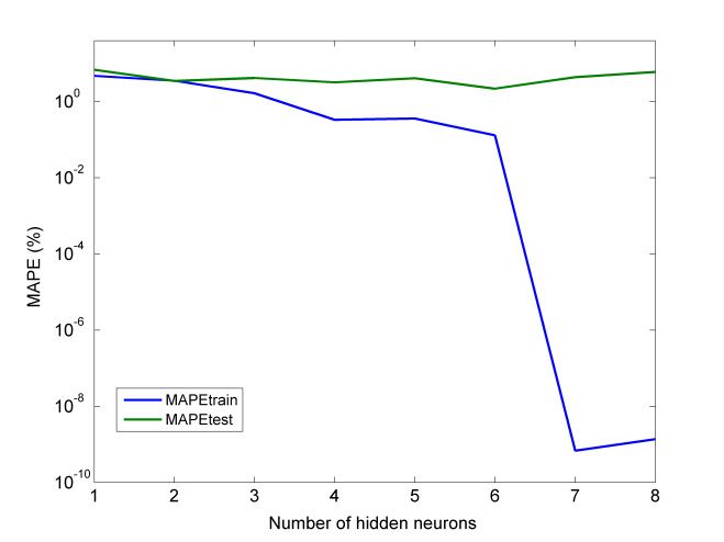
Machines 2019, 7, 13                                                                                      9 of 18

  Machines 2019, 7, x FOR PEER REVIEW                                                                   9 of 19

4. Results and Discussion
  4. Results and Discussion
4.1. Result of Experiment
  4.1. Result of Experiment
      Figure 5 shows the experimental values derived from the whole process. It is clear that there
        Figure 5 shows the experimental values derived from the whole process. It is clear that there was
was a relationship between cutting parameters and cutting forces. When the tool diameter increased,
  a relationship between cutting parameters and cutting forces. When the tool diameter increased, both
both cutting forces increased. As the feed rate values increased, the cutting forces increased respectively.
  cutting forces increased. As the feed rate values increased, the cutting forces increased respectively.
The cutting speed did not noticeably affect either cutting force. A full factorial strategy was applied,
  The cutting speed did not noticeably affect either cutting force. A full factorial strategy was applied,
and twenty seven (27) drilling experiments were performed, while both Fz and Mz were modelled
  and twenty seven (27) drilling experiments were performed, while both Fz and Mz were modelled
separately
  separatelyusing
              usingpolynomial
                     polynomialmathematical
                                mathematicalmodels.
                                               models.

                             Figure5.5.Experimental
                            Figure     Experimental values
                                                    values derived
                                                           derived from
                                                                   from Kistler
                                                                        Kistler 9123.
                                                                                9123.

4.2.
  4.2.Multiple
       MultipleRegression
                RegressionModels
                          Models
      The
       TheRSMRSMisisa atool
                        toolbased
                             basedononthe
                                        thecollection
                                            collection of
                                                        of statistical
                                                           statistical and mathematical
                                                                            mathematical techniques
                                                                                           techniquesused
                                                                                                        usedfor
                                                                                                             for
process
  processoptimization.
           optimization.Optimization
                            Optimization can
                                           can be
                                               be managed
                                                   managed by creating      an empirical
                                                                  creating an  empirical relationship
                                                                                          relationshipbetween
                                                                                                        between
independent
  independentvariables
                variablesand andthe
                                 the response
                                      response ofof the
                                                     the system
                                                         system using thethe quantitative
                                                                             quantitative data
                                                                                           datacollected
                                                                                                 collectedfrom
                                                                                                           from
  experiment[5,6].
experiment     [5,6].
                    TheThe    experiments
                         experiments    werewere    designed
                                             designed           and executed
                                                         and executed            by employing
                                                                         by employing             second-order
                                                                                        second-order   nonlinear
  nonlinear mathematical
mathematical    models in models
                              order toinpredict
                                         order tothe
                                                  predict
                                                      thrustthe thrust
                                                              force andforce
                                                                         theand  the cutting
                                                                              cutting torque,torque,
                                                                                               whichwhich
                                                                                                      are ofare
                                                                                                             the
  of the following
following form:     form: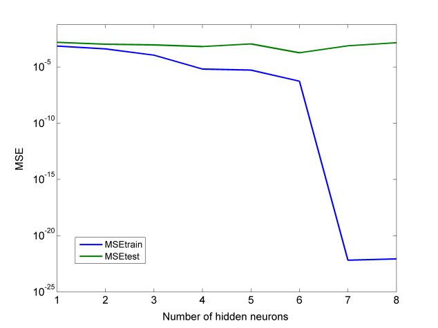
Machines 2019, 7, 13                                                                                    10 of 18

           Y = b0 + b1 X1 + b2 X2 + b3 X3 + b4 X12 + b5 X22 + b6 X32 + b7 X1 X2 + b8 X1 X3 + b9 X2 X3       (5)

where Y is the response, Xi stands for the coded values, and bi stand for the models’
regression coefficients.
     When the level of significance is very small, less than 0.05, this indicates that the results were
high and probably not randomly scattered. The significant terms were found by Analysis Of Variance
(ANOVA) for each response (Tables 3 and 4).

                                  Table 3. ANOVA table for Fz (thrust force).

             Source          Degree of Freedom     Sum of Squares      Mean Square     f -Value   p-Value
         Regression                   9                514.673              57.186     471.95      0.000
       Residual Error                17                 2060                 121
            Total                    26                516.733
      R-Sq(adj) = 99.4%
                            Parameter Estimate
           Predictor                                  Standard Error Coefficient       t-Value    p-Value
                                Coefficient
           Constant               −221.9                           151.4               −1.47       0.161
              D                    57.59                           23.60               2.44        0.026
               V                  1.9550                          0.5455               3.58        0.002
               f                   1291.8                          798.0               1.62        0.124
             D*D                  −0.762                           1.123               −0.68       0.506
             V*V                 −0.011660                       0.001798              −6.49       0.000
              f*f                  −667                            1798                −0.37       0.715
             D*V                  0.05600                        0.03178               1.76        0.096
             D*f                  103.25                           31.78               3.25        0.005
             V*f                  −1.203                           1.271               −0.95       0.357

                                    Table 4. ANOVA table for Mz (torque).

             Source          Degree of Freedom     Sum of Squares      Mean Square     f -Value   p-Value
         Regression                   9                37.8929              4.2103     171.77      0.000
       Residual Error                17                 0.0924              0.0245
            Total                    26                38.3096
      R-Sq(adj) = 98.3%
                            Parameter Estimate
           Predictor                                  Standard Error Coefficient       t-Value    p-Value
                                Coefficient
           Constant               12.941                         2.154                 6.01        0.000
              D                  −2.6736                         0.3357                −7.96       0.000
               V                 0.013678                      0.007758                1.76        0.096
               f                  −15.58                         11.35                 −1.37       0.188
             D*D                  0.14025                       0.01598                8.78        0.000
             V*V                −0.00005493                   0.00002557               −2.15       0.046
              f*f                   4.67                         25.57                 0.18        0.857
             D*V                −0.0001225                    0.0004520                −0.27       0.790
             D*f                  2.6250                         0.4520                5.81        0.000
             V*f                 −0.02330                       0.01808                −1.29       0.215

     The following regression equations for the thrust force and the cutting torque as a function of
three input process variables were developed:

           Fz = − 222 + 57.6 D + 1.96 V + 1292 f – 0.76 D ∗ D – 0.0117 V ∗ V − 667 f ∗ f
                                                                                                            (6)
           + 0.0560 D ∗ V + 103 D ∗ f – 1.20 V ∗ f
The following regression equations for the thrust force and the cutting torque as a function of
three input process variables were developed:
Fz = − 222 + 57.6 D + 1.96 V + 1292 f ? 0.76 D * D ? 0.0117 V * V − 667 f * f
(6)
+ 0.0560 D * V + 103 D * f ? 1.20 V * f ?
Machines 2019, 7, 13 11 of 18
and:
and:
M z = 12.9 ? 2.67 D + 0.0137 V ? 15.6 f + 0.140 D * D ? 0.000055 V *V + 4.7 f * f
(7)
牋
M牋−z =0.000122
12.9 −D2.67*V + D 2.63 D * f V? −
+ 0.0137 0.0233
15.6 Vf *+f ?0.140 D ∗ D − 0.000055 V ∗ V + 4.7 f ∗ f
(7)
− 0.000122 D ∗ V + 2.63 D ∗ f − 0.0233 V ∗ f
where D is the tool diameter (mm), f is the feed rate (mm/rev), and V is the cutting speed (m/min).
where D is the tool diameter (mm), f is the feed rate (mm/rev), and V is the cutting speed (m/min).
The p-values
The p-values areareused
usedasasa basic tooltool
a basic to check
to checkthe importance
the importance of eachof of the of
each coefficients. The smaller
the coefficients. The
the amount of P, the more significant is the corresponding coefficient.
smaller the amount of P, the more significant is the corresponding coefficient. In our case, In our case, for F z for Fzfactors
, these , these
are: D (p-value
factors are: D= 0.026),
(p-valueV (p-value
= 0.026),= 0.002), V*V (p-value
V (p-value = 0.000),
= 0.002), V*Vand(p-value
D*f (p-value = 0.005),and
= 0.000), whileD*ffor
M z , the
(p-value significant terms are: D (p-value = 0.000), D*D (p-value = 0.000), V*V (p-value
= 0.005), while for Mz, the significant terms are: D (p-value = 0.000), D*D (p-value = 0.000), =0.046), and D*f
(p-value
V*V (p-value = 0.000).
=0.046),Moreover, from Tables
and D*f (p-value 3 and
= 0.000). 4, it is from
Moreover, evaluated
Tablesthat the4,coefficient
3 and it is evaluated of multiple
that the
determination was very close to unity for both cases (R 2 = 99.6% for F and R2 = 98.9% for M ), and the
coefficient of multiple determination was very close to unity for both cases (R = 99.6% for z 2 z Fz and
adjusted
R 2 = 98.9% coefficient (R2 adj)
for Mz), and was 99.4%
the adjusted for Fz and(R98.3%
coefficient 2 adj) for
wasM99.4%
z . All these
for Fzstatistical
and 98.3% estimators
for Mz. All indicate
these
an appropriate RSM model with the degree of freedom and optimal
statistical estimators indicate an appropriate RSM model with the degree of freedom and optimal architecture that can be used for
predictive simulations of the reactive extraction. Of course, for both cases,
architecture that can be used for predictive simulations of the reactive extraction. Of course, for both only the significant terms
can beonly
cases, included in order toterms
the significant presentcanabe
setincluded
of simplified equations.
in order to presentTheaagreement between
set of simplified experimental
equations. The
and RSM predicted data is shown in Figure 6. Residual analysis was
agreement between experimental and RSM predicted data is shown in Figure 6. Residual analysis performed to test the models’
accuracy;
was performedin bothto cases,
test theallmodels’
points were positioned
accuracy; in bothnear
cases,to all
a straight line, indicating
points were positionedthat nearRSM predicts
to a straight
the experimental
line, indicating that data
RSMforpredicts
the considered valid region
the experimental well.
data for the considered valid region well.
Figure 6. Residuals analyses for Fzz and
Figure 6. and M
Mz.z.
4.3. Multi-Layer
4.3. Multi-Layer Perceptron
Perceptron Models
Models
As was
As was described
described ininthe
theMethods
MethodsandandMaterials
Materialssection,
section,in in
thethe
casecase of MLP
of MLP models,
models, an
an investigation of the optimum number of hidden neurons was conducted based on various
investigation of the optimum number of hidden neurons was conducted based on various criteria. criteria.
After the
After the MLP
MLP models
models were
were developed,
developed, the
the results
results obtained
obtained were
were asas presented
presented in
in Table
Table 5.
5.
Table 5. Results regarding the MLP models for thrust force (Fz ).
No. of Hidden Neurons MSEtrain MSEtest MAPEtrain (%) MAPEtest (%)
1 2.35 × 10⁻⁴ 6.36 × 10⁻⁴ 1.46 × 100 2.93 × 100
2 8.42 × 10⁻⁵ 1.05 × 10⁻⁴ 9.84 × 10⁻¹ 1.14 × 100
3 2.72 × 10⁻⁷ 1.53 × 10⁻⁴ 5.32 × 10⁻² 1.36 × 100
4 2.20 × 10⁻⁶ 6.10 × 10⁻⁵ 1.36 × 10⁻¹ 8.23 × 10⁻¹
5 1.78 × 10⁻¹⁵ 1.31 × 10⁻⁴ 2.50 × 10⁻⁶ 9.45 × 10⁻¹
6 3.40 × 10⁻²² 4.42 × 10⁻⁴ 2.04 × 10⁻⁹ 2.22 × 100
7 4.98 × 10⁻²⁴ 2.59 × 10⁻⁴ 2.12 × 10⁻¹⁰ 2.02 × 100
8 5.03 × 10⁻²³ 2.60 × 10⁻⁴ 6.41 × 10⁻¹⁰ 2.06 × 100
As can be seen from Table 5 and Figure 7, in the case of the thrust force model, the MSE for
the training dataset was generally decreasing with an increase of the number of hidden neurons.
Especially, for models with over five neurons, the MSE became extremely small, indicating that the7 4.98 × 10⁻²⁴ 2.59 × 10⁻⁴ 2.12 × 10⁻¹⁰ 2.02 × 100
8 5.03 × 10⁻²³ 2.60 × 10⁻⁴ 6.41 × 10⁻¹⁰ 2.06 × 100
As can be seen from Table 5 and Figure 7, in the case of the thrust force model, the MSE for the
Machines
training2019, 7, 13
dataset was generally decreasing with an increase of the number of hidden neurons. 12 of 18
Especially, for models with over five neurons, the MSE became extremely small, indicating that the
training dataset can be reproduced with a high level of accuracy by this model. However, the MSE
training dataset can be reproduced with a high level of accuracy by this model. However, the MSE
for the testing dataset, which is an indication of overfitting, became the minimum for the model with
for the testing dataset, which is an indication of overfitting, became the minimum for the model with
four hidden neurons and then increased again. A similar situation was observed in the case of MAPE,
four hidden neurons and then increased again. A similar situation was observed in the case of MAPE,
where MAPE for the training dataset became extremely small for networks with more than four
where MAPE for the training dataset became extremely small for networks with more than four hidden
hidden neurons, but the minimum MAPE for the testing dataset was obtained for the model with five
neurons, but the minimum MAPE for the testing dataset was obtained for the model with five hidden
hidden neurons. Thus, the optimum number of hidden neurons was four or five, and the final choice
neurons. Thus, the optimum number of hidden neurons was four or five, and the final choice was
was conducted in terms of total error, as the error values for these cases were very close. Finally, the
conducted in terms of total error, as the error values for these cases were very close. Finally, the case
case with four neurons was chosen as the total error was very close to the total error of the case with
with four neurons was chosen as the total error was very close to the total error of the case with five
five neurons, and this network was less complex than the other.
neurons, and this network was less complex than the other.
(a) (b)
Figure7.7.Results
Figure Resultsregarding
regardingthe
theMLP
MLPmodel
modelfor
forFzF:z:(a)
(a)MSE
MSEfor
fortraining
trainingand
andtesting
testingdatasets,
datasets,(b)
(b)MAPE
MAPE
fortraining
for trainingand
andtesting
testingdatasets.
datasets.
AsAscan
canbe beseen
seenfrom
fromTable
Table6 6and
andFigure
Figure8,8,ininthe
thecase
caseofofthe
thetorque
torquemodel,
model,thetheMSEMSEforfortraining
training
was
wasdecreasing
decreasingwith withan anincreasing
increasingnumber
numberofofhidden
hiddenneurons,
neurons,mainly
mainlyfor formodels
modelswithwithmore
morethanthansixsix
hidden
hiddenneurons.
neurons.However,
However,the theminimum
minimumvalue valueofofMSEMSEforforthethetesting
testingdataset
datasetwaswasobtained
obtainedfor forthe
the
model
modelwith
withfour
fourhidden
hiddenneurons.
neurons.Regarding
RegardingMAPE,
MAPE,the theminimum
minimumvalue valueforforthe
thetraining
trainingdataset
datasetwas was
obtained
obtainedforfor
thethe
model
model with seven
with hidden
seven neurons,
hidden whereas
neurons, the minimum
whereas value for
the minimum the testing
value for thedataset
testing
was obtained
dataset for the model
was obtained with
for the six hidden
model with six neurons.
hidden Thus,
neurons.the Thus,
best model
the bestwasmodel
determined again by
was determined
checking
again bythe total error,
checking the and
totaliterror,
was determined
and it was that the network
determined that with six hidden
the network withneurons was the
six hidden best
neurons
performing
was the bestone. Generally,one.
performing it was observed
Generally, it that
was the error values
observed that the forerror
the M z model
values for were
the Mconsiderably
z model were
larger than those
considerably of the
larger thanFzthose
model. Nevertheless,
of the the results confirmed
Fz model. Nevertheless, the resultsthat the optimum
confirmed number
that the optimum of
neurons
numberwas dependent
of neurons was on the size of
dependent onthe
thedataset;
size of theas for the relatively
dataset; as for thesmall dataset
relatively of 27
small samples,
dataset of 27
a samples,
model with six hidden
a model with sixneurons
hidden was sufficient.
neurons was sufficient.
Table 6. Results regarding the MLP models for torque (Mz ).
No. of Hidden Neurons MSEtrain MSEtest MAPEtrain (%) MAPEtest (%)
1 7.39 × 10⁻⁴ 1.57 × 10⁻³ 4.75 × 100 6.86 × 100
2 4.11 × 10⁻⁴ 1.08 × 10⁻³ 3.53 × 100 3.48 × 100
3 1.14 × 10⁻⁴ 9.34 × 10⁻⁴ 1.65 × 100 4.15 × 100
4 6.65 × 10⁻⁶ 6.66 × 10⁻⁴ 3.32 × 10⁻¹ 3.20 × 100
5 5.36 × 10⁻⁶ 1.14 × 10⁻³ 3.59 × 10⁻¹ 4.10 × 100
6 5.53 × 10⁻⁷ 1.86 × 10⁻⁴ 1.30 × 10⁻¹ 2.19 × 100
7 6.60 × 10⁻²³ 7.81 × 10⁻⁴ 6.79 × 10⁻¹⁰ 4.36 × 100
8 8.68 × 10⁻²³ 1.45 × 10⁻³ 1.36 × 10⁻⁹ 6.01 × 1004 6.65 × 10⁻⁶ 6.66 × 10⁻⁴ 3.32 × 10⁻¹ 3.20 × 100
5 5.36 × 10⁻⁶ 1.14 × 10⁻³ 3.59 × 10⁻¹ 4.10 × 100
6 5.53 × 10⁻⁷ 1.86 × 10⁻⁴ 1.30 × 10⁻¹ 2.19 × 100
7 6.60 × 10⁻²³ 7.81 × 10⁻⁴ 6.79 × 10⁻¹⁰ 4.36 × 100
8 8.68 × 10⁻²³ 1.45 × 10⁻³ 1.36 × 10⁻⁹ 6.01 × 100
Machines 2019, 7, 13 13 of 18
(a) (b)
Figure
Figure 8. Results
8. Results regarding
regarding thethe
MLPMLP model
model forfor
MM : (a)MSE
z : z(a) MSEfor
forthe
the training
training and testing
testing datasets
datasetsand
and
(b) MAPE for the training and testing datasets.
(b) MAPE for the training and testing datasets.
4.4. 4.4.
Radial Basis
Radial Function
Basis Neural
Function Network
Neural Models
Network Models
As was
As waspreviously
previously mentioned,
mentioned, ininthethecase
caseofofRBF-NN
RBF-NNmodels,models, it
it is
is intended
intended to to determine
determinethe the
optimum
optimumnumber
number of hidden
of hiddenneurons.
neurons. InInTable
Table 3,3,the
theresults
resultsfrom
fromthe
theRBF-NN
RBF-NN models are are presented.
presented.
For For
the the
RBF-NN
RBF-NN models
modelsin in
thethe
case
case ofofthrust
thrustforce,
force,ititcan
canbe
be observed
observed fromfrom Table
Table77and andFigure
Figure9 9
thatthat
MSE MSE
for for
thethe training
training setset
waswas decreasingwith
decreasing withan anincreasing
increasingnumber
number of hidden
hidden neurons,
neurons,but butthere
there
waswasnot not
suchsuch a large
a large decrease
decrease as as
in in
thethe case
case ofofMLP
MLPmodels.
models.For For the
the testing
testing dataset,
dataset, MSE MSEwas wasthe the
minimum for the model with seven hidden neurons, and the same was
minimum for the model with seven hidden neurons, and the same was noted for MAPE for the training noted for MAPE for the
training
dataset. dataset.
Thus, Thus,with
the model the model
seven with
hidden seven hidden
neurons neurons
was was thein
the optimum optimum inItthis
this case. case.
is to It is to that
be noted be
noted of
the value that the value
MAPE of MAPE
for both for bothand
the training the testing
trainingdataset
and testing dataset was considerably
was considerably reduced for reduced
models withfor
models with over three neurons, something that was not observed to a similar
over three neurons, something that was not observed to a similar extent in the case of MLP models, extent in the case of
MLP models, at least for the testing dataset.
at least for the testing dataset.
Table 7. Results regarding the RBF-NN models for thrust force (Fz).
Table 7. Results regarding the RBF-NN models for thrust force (Fz ).
No. of Hidden Neurons MSEtrain MSEtest MAPEtrain(%) MAPEtest(%)
No. of Hidden Neurons MSEtrain MSEtest MAPEtrain (%) MAPEtest (%)
1 9.92 × 10⁻³ 2.01 × 10 −2 1.08 × 10⁻¹ 1.94 × 10¹¹
1 9.92 × 10⁻³ 2.01 × 10⁻²−4 1.08 × 10⁻¹ 1.94 × 10
2 1.20 × 10⁻³ 6.62 × 10 4.09 × 1000 2.70 × 1000
2 1.20 × 10⁻³ 6.62 × 10⁻⁴ 4.09 × 10 2.70 × 10
3 3 1.59 × 10−×
1.59 4 10−4 2.78××1010
2.78 −4−4 1.34
1.34 ××10
0
100 1.98
1.98 ×
× 10
100
0
− 4 −4−4 1000 1000
4 4 1.30
1.30 × 10 × 10−4 1.39××1010
1.39 1.21
1.21 ××10 1.51
1.51 ×
× 10
5 9.99 × 10 −5 1.60 × 10 −4 1.12 × 1000 1.52 × 1000
5 9.99 × 10⁻⁵ 1.60 × 10⁻⁴ 1.12 × 10 1.52 × 10
6 9.07 × 10⁻⁵ 1.65 × 10⁻⁴−4 1.02 × 1000 1.45 × 1000
Machines 2019, 7, x FOR 6 9.07 × 10⁻⁵
7 PEER REVIEW8.19 × 10−5
1.65 × 10
1.14 × 10⁻⁴
1.02 × 10
9.42 × 10⁻¹
1.45 × 10
1.13 × 100 14 of 19
8 7 8.19
7.67 × 10−× 5 10−5 1.14××1010
1.32 −4−4 9.42
9.29 ×10
× −1
10−1 1.13
1.35 ×
× 10
100
0
8 7.67 × 10⁻⁵ 1.32 × 10⁻⁴ 9.29 × 10⁻¹ 1.35 × 100
(a) (b)
Figure
Figure 9. Results
9. Results regarding
regarding thethe RBF-NN
RBF-NN model
model forfor
Fz :F(a)
z: (a)
MSEMSE
forfor training
training and
and testing
testing datasets
datasets and(b)
and
(b) MAPE
MAPE for training
for training and testing
and testing datasets.
datasets.
As for the torque (Mz) cases, it was observed from Table 8 and Figure 10 that the optimum model
was the one with eight hidden neurons, as it exhibited both a lower MSE and MAPE for the testing
dataset. Thus, it can be stated that for RBF-NN models, a slightly larger number of hidden neurons
was required compared to MLP models.(a) (b)
Figure 9. Results regarding the RBF-NN model for Fz: (a) MSE for training and testing datasets and
(b) MAPE for training and testing datasets.
Machines
As2019, 7, 13torque (Mz) cases, it was observed from Table 8 and Figure 10 that the optimum 14
for the of 18
model
was the one with eight hidden neurons, as it exhibited both a lower MSE and MAPE for the testing
dataset. Thus,
As for it can be
the torque (Mstated that for RBF-NN models, a slightly larger number of hidden neurons
z ) cases, it was observed from Table 8 and Figure 10 that the optimum model
was required compared to MLP models.as it exhibited both a lower MSE and MAPE for the testing
was the one with eight hidden neurons,
dataset. Thus, it can be stated that for RBF-NN models, a slightly larger number of hidden neurons
Table 8. Results regarding the RBF-NN models for torque (Mz).
was required compared to MLP models.
No of Hidden Neurons MSEtrain MSEtest MAPEtrain(%) MAPEtest(%)
1Table 8. Results3.31
regarding
× 10−2 the5.94
RBF-NN
× 10−2models3.03
for torque
× 101 (Mz ). 3.60 × 101
2
No of Hidden Neurons 5.60 × 10⁻³ 1.26
MSEtrain × 10−2
MSEtest 1.37 × 101 (%) 2.13
MAPEtrain × 101 (%)
MAPEtest
3 4.20 × 10 −3 1.05 × 10 2
−2 1.14 × 10 11 1.98 × 101 1
1 3.31 × 10⁻² −3 5.94 × 10− 3.03 × 10 3.60 ×1 10
2
4 2.74 × 10
5.60 × 10⁻³
1.05 × 10⁻²
1.26 × 10⁻²
9.511.37
× 10 0
× 101
2.042.13
× 10× 101
3 5 2.65
4.20 × 10 × 10
− 3 −3 1.23 × 10
1.05 × 10
−2
− 2 9.521.14
× 10 0
× 10 1 2.381.98
× 10×1 101
4 6 2.37
2.74 × − 3
10 × 10 −3 7.83 × 10
1.05 × −
−32 9.209.51
× 10 0
× 10 0 × 10×1 101
1.832.04
− 3 − 2 0
5 7 2.65 ×
6.49 1.23 ×
10 × 10−4 1.24 × 10⁻³ 4.639.52 ×0 10
× 10 × 10×0 101
6.272.38
2.37 × − 3 7.83 × − 3 ×0 10 0 1
6 8 10 × 10−4 8.73
4.82 −4
10 −4
× 10 −3
3.759.20
× 10 0
× 10×0 100
5.811.83
7 6.49 × 10 1.24 × 10 4.63 × 10 6.27 × 10
8 4.82 × 10⁻⁴ 8.73 × 10⁻⁴ 3.75 × 100 5.81 × 100
(a) (b)
Figure10.
Figure 10.Results
Resultsregarding
regardingthe
theRBF
RBFmodel
modelforfor
MzM z: (a)
: (a) MSEMSE
forfor training
training andand testing
testing datasets
datasets andand
(b)
(b) MAPE
MAPE for training
for training and and testing
testing datasets.
datasets.
4.5. Adaptive Neuro-Fuzzy Inference System Models
In the case of ANFIS models, results from cases with a different number of clusters are presented
in Table 9.
Table 9. Results regarding the ANFIS models for thrust force (Fz ).
No of Clusters MSEtrain MSEtest MAPEtrain (%) MAPEtest (%)
2 4.94 ×10⁻⁵ 3.68 ×10⁻⁴ 8.03 × 10⁻¹ 2.49 × 100
3 1.37 × 10⁻⁵ 4.47 × 10⁻⁴ 3.60 × 10⁻¹ 2.74 × 100
4 2.80 × 10⁻⁶ 1.20 × 10⁻⁴ 1.40 × 10⁻¹ 1.07 × 100
In the case of the ANFIS models for thrust force, it can be seen from Table 9 and Figure 11 that
the MSE for both training and testing datasets was reduced with an increasing number of clusters.
Furthermore, the same can be observed for the MAPE for both datasets; thus, the ANFIS model with
four clusters was selected as the best performing network. In the case of torque models, whose results
are presented in Table 10 and Figure 12, the optimum value of MSE for the testing dataset was obtained
for the model with two clusters, whereas the optimum value of MAPE for the testing dataset was
obtained for the model with four clusters. Therefore, the best model was selected according to the total
error values, which were lower for the model with four clusters.You can also read