Stratified-Extended Cox with Frailty Model for Non-Proportional Hazard: A Statistical Approach to Student Retention Data from Universitas Terbuka ...
←
→
Page content transcription
If your browser does not render page correctly, please read the page content below
Thailand Statistician
                  January 2021; 19(1): 209-228
                  http://statassoc.or.th
                  Contributed paper

Stratified-Extended Cox with Frailty Model for Non-Proportional
Hazard: A Statistical Approach to Student Retention Data from
Universitas Terbuka in Indonesia
Dewi Juliah Ratnaningsih*[a], Asep Saefuddin [b], Anang Kurnia [b],
I Wayan Mangku [c]
[a] Department of Statistics, Faculty of Mathematics and Natural Sciences, Universitas Terbuka,
    South Tangerang, Indonesia.
[b] Department of Statistics, Faculty of Mathematics and Natural Sciences, IPB University, Bogor,
    Indonesia.
[c] Department of Mathematics, Faculty of Mathematics and Natural Sciences, IPB University,
    Bogor, Indonesia.
*Corresponding author; e-mail: djuli@ecampus.ut.ac.id

                                                                                   Received: 4 June 2019
                                                                                 Revised: 18 August 2019
                                                                                 Accepted: 20 March 2020

Abstract
     This paper aims to describe new modelling to overcome the problem of non-proportional hazard
modelling in survival analysis. One cause of non-proportional hazard is the presence of time-
dependent covariates and the presence of frailty. The proposed model is called the stratified extended
with frailty (SEF) model. The method used in estimating model parameters is the hierarchical
likelihood. The goodness of the model is tested by simulating utilizing the R program. The criteria
used are parameter bias and Mean Squared Error. The developed model is applied to the Universitas
Terbuka student retention data. The results of the study show that covariates that significantly affect
the survival of the students of UT in their course of study are: educational background, age, GPA,
marital status, the number of credit hours they completed, and the number of classes they have taken
in each semester. Based on other similar studies, this is a common condition that occurs in other
countries where some educational institutions apply the distance education system.

Keywords: Analysis survival, hierarchical likelihood, time-dependent covariate, random effect, frailty model.

1.   Introduction
     Survival analysis is one of the methods of analysis in statistics which is performed to model
survival time that involves a number of predictor variables (covariates). The primary factor that
distinguishes survival analysis from other methods of statistical analyses is the presence of censored
observation. Most survival analyses must consider a key analytical problem called censoring. A
censored observation occurs when we have some information about individual survival time, but we
don’t know the survival time exactly. Lee and Wang (2003) explain that censored data indicate a
situation when part of the required data in a research process is unobtainable because there is an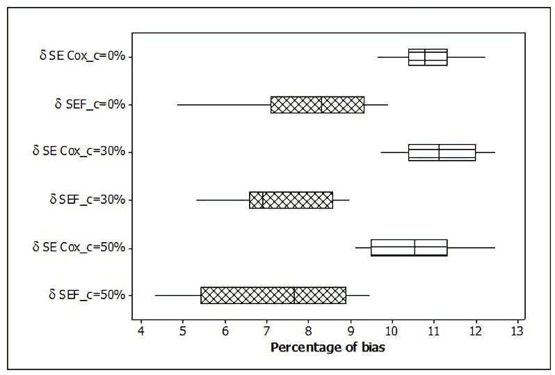
210                                                        Thailand Statistician, 2021; 19(1): 209-228

individual under study who either has not experienced the observed occurrence or has not finished
receiving the given treatment by the end of the research. It may happen, for example, with a cancer
patient when he has to be transferred to another hospital or passes away during particular time interval
that he is no longer available for observation. Censored observation may also occur in the area of
research related to education, particularly in a kind of case with researches involving college students
as the subjects, when the students under observation drop out or transfer to another university.
Dropout and transfer are two of the typical occurrences in higher education sphere that cause students’
academic records to be incomplete or overlooked.
     One of the models which are commonly adopted to assess survival time with the involvement of
censored observation is Cox model. Cox model assumes that each individual’s hazard rate is
proportional to other individuals’ hazard rates with constant ratio at all times. For this reason, Cox
model is also known as Cox proportional hazard. In practice, however, this assumption is frequently
unsubstantiated, especially when there are time-dependent covariates involved. The presence of time-
dependent covariates creates a condition characterized by disproportional individuals’ hazard rates
for which the course of time is the affecting factor. This condition is known as non-proportional
hazard.
     One other factor that contributes to non-proportional hazard is the presence of unobserved
random effect. Some statisticians perceive that the presence of unobserved covariates is likely
associated with heterogeneity of data. Unobserved covariates in a survival model are identified as
frailty (Vaupel et al. 1979). The guiding assumption of survival analysis is that the population under
observation is homogenous, but when frailty is present, heterogeneity in the population will appear
as the consequence.
     Wienke (2011) argues that in some cases, a researcher needs to take into account the
heterogeneity element of her sample as indicated in her research population from which the sample
is taken. It is important because sample heterogeneity may disrupt the assumption that underlies Cox
model. The violation of proportional hazard’s assumption causes inaccuracy in parameter estimation
and standard error (Henderson and Oman 1999). In that case, the occurrence of any individual’s
hazard rate that is not proportional (non-proportional hazard) needs to be treated properly to ensure
that a modelling function can be particularly useful and generate parameter estimation that is most
representative of the actual condition.
     Non-proportional hazard that is caused by the presence of both time-independent covariates and
time-dependent covariates can be resolved by combining two methods called stratified Cox and
extended Cox. Ratnaningsih et al. (2019) has carried out a study in which they apply the two models
in tandem. The combination is called stratified extended Cox (SE Cox) and has been applied to data
from student records at Universitas Terbuka (UT). In survival analysis, hazard function for each
individual depends on the observed covariates. However, in some cases, some of the involving
covariates are unknown or indeterminate. An unobserved covariate, which is identified as random
effect, is called frailty. As mentioned previously, frailty invalidates Cox model’s assumption.
     The present paper aims to develop a survival model for non-proportional hazard which is associated
with time-independent covariate, time-dependent covariate and frailty. The suggested model is named
as stratified extended Cox model with frailty (SEF model). This model is expected to be applicable to
data related to issues in education, particularly the survival data of the students at UT.
     Universitas Terbuka is one of higher educational institutions which mainly provide distance
education. The periods of study at UT vary due to several factors. Those factors or covariates can be
categorized into time-independent covariates and time-dependent covariates (Ratnaningsih et al.
2019). The characteristics of the students of the university also vary, and therefore it is highly likely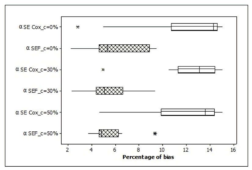
Dewi Juliah Ratnaningsih et al. 211
that the data related to them and their study at the university will be heterogenous. One of the causes
of heterogeneity in data is the involvement of unobserved covariates known as frailty. Thus, the
application of SEF model to the data related to the students of UT is considered suitable. The
application of the model in this case is aimed at producing a more meaningful statistical modelling
with which parameter estimation that is most representative of the actual condition can be achieved.
2. Stratified-Extended Model with Frailty
2.1. The proposed model
Stratified extended model with frailty (abbreviated as SEF model for this paper) is proposed in
this study to address non-proportional hazard cases effectively. This model is the outgrowth of the
previously developed model known as stratified extended Cox (SE Cox) that has been presented by
Ratnaningsih et al. (2019) in their study. Their study has shown that SE Cox model is able to resolve
non-proportional hazard in a survival model that involves time-dependent covariates.
The central difference between SE Cox and SEF model is marked by the presence of unobserved
random effect in the latter, which is known as frailty (Vaupel et al. 1979). As an unobserved random
effect, frailty is capable of altering the hazard function of an individual or group of individuals as
well as an individual who undergoes recurring event(s). Non-proportional hazard in SEF model
occurs because of the presence of time-independent covariates, time-dependent covariates and frailty.
The underlying assumption that generates the notion of frailty is that each individual has his/her
own weaknesses that differentiate him/her from other individuals, the kind of factor that can create
heterogeneity. The assumption suggests that the frailest individual will be the earliest to die compared
to other individuals in the same group (Therneau et al. 2003). Thus, frailty is a significant contributor
to such heterogeneity. On the contrary, the basic assumption in survival analysis is that the observed
population is homogenous. Therefore, the proposed model in this case is intended to manage the
involvement of frailty, time-independent covariates and time-dependent covariates that are associated
with non-proportional hazard.
SEF model is mathematically defined as follows.
p1 p2
s (t , x ) 0 s (t ) exp ai xai bi xbi (t j ) vs , (1)
a 1 b 1
where
s = the order of stratum; s 1, 2,..., m (denoting the number of strata combination),
0 s (t ) = baseline hazard function on each stratum,
ai = fixed effect coefficient vector for covariate number a of individual number i,
xai = time-independent covariate (fixed effect) number a of individual number i,
bi = coefficient vector for time-dependent covariate number b of individual number i,
xbi (t j ) = time-dependent covariate of individual number i at time t j ,
= frailty coefficient vector,
vs = frailty on stratum number s.
2.2. Parameter estimation in the model
Parameter estimation used in SEF model is based on likelihood. In its application, the estimation
is performed according to a procedure called hierarchical likelihood (H-likelihood) proposed by
Ha et al. (2001) and Ha et al. (2019) with log-normal frailty distribution.
Using (1), these following derivatives can be made: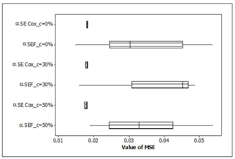
212 Thailand Statistician, 2021; 19(1): 209-228
p1 p2
si ai xai bi xbi (t j ),
a 1 b 1
p1 p2
si ai xai bi xbi (t j ) vs ,
a 1 b 1
where Tsi ( s 1, 2,..., m, i 1, 2,..., ns ) denotes the survival time for individual number i on stratum
number s and Csi represents the censored time for individual i on stratum number s. Accordingly,
the observed data is expressed as ysi min (Tsi , Csi ) and si I (Tsi Csi ) where I (.) is an indicator
function. The value of this indicator function is 1 for the censored data and 0 for the non-censored
data and vs signifies unobserved log-frailty. If us denotes unobserved random variable (frailty) on
stratum number s, then vs log us . Ha et al. (2001) and Ha et al. (2019) represent frailty with these
following assumptions.
1. Assumption 1: It is given that U i ui ,{(Tsi , Csi ), i 1, 2,..., ns } is independent, and it follows
that Tsi and Csi are also independent for s 1, 2,..., m; i 1, 2,..., ns .
2. Assumption 2: It is given that U i ui ,{(Tsi , Csi ), i 1, 2,..., ns } is considered non-informative
with respect to us .
In this paper, it is assumed that us ~ LN (0, ) so that vs ~ N (0, ). It is supported by these
aspects:
1. us ~ LN (0, ), vs log us vs ~ N (0, ).
2. vs ~ N (0, ), us evs us ~ LN (0, ).
If ys ( ys1 ,..., ysns )T and s ( s1 ,..., sns )T , then hierarchical likelihood, which is denoted by h,
is to be defined as the sum of hs , s 1, 2,..., m. Hence we have
h s hs , (2)
where hs denotes the algorithm of shared density ( ys , s , vs ).
Furthermore h s can be represented by the equation below
hs ( , , s , ; ys , s , vs ) log{L1s ( , , s ; ys , s | us ) L2 s ( ; vs )}, (3)
where
L1s = conditional density of ( ys , s ) with us as the condition,
L2s = density of vs .
Since L1s is assumed as an independent variable in (3), it can be further represented in this
following formula
L1s ( , , s ; ys , s | us ) L1si ( , , s ; ys , s | u s ), (4)
i
where
L1si = conditional density of ( ysi , si ) with us as the condition.
L1si from (4) can be expressed in (5) below
L1s ( , , s ; ys , s | us ) ( ysi | us ) si exp{( ysi | us )}. (5)
i
Furthermore, if it is assumed that vs ~ N (0, ), then L2s from (3) can be formulated in (6) below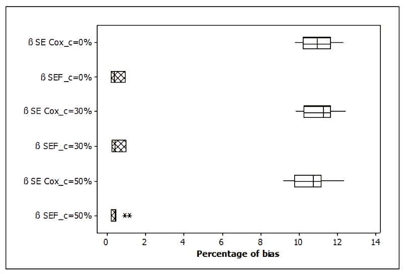
Dewi Juliah Ratnaningsih et al. 213
1
1
L2 s ( ; vs ) (2 ) 2
exp vs2 , vs . (6)
2
Thus, if (5) and (6) are incorporated into (3), the resulting formulation appears as follows
1 1
hs ( si {log{0 s ( ysi )) si } { 0 s ( ysi ) exp( si )}) log (2 ) vs2 . (7)
i 2 2
Moreover, by incorporating h s hs , (2) can be rewritten as follows
h h ( , , v, 0 s , ) hs ,
s
(8)
m 1
si log 0 s ( ysi ) si 0 s ( ysi ) exp( si ) log (2 ) vs2 .
si 2 2 s
Furthermore, if log L1si si log 0 s ( ysi ) si 0 s ( ysi ) exp( si ) in (8) is denoted by l1si ,
1 1 2
and log L2 s log (2 ) vs is denoted by l2s , then the following formula is obtained (Ha
2 2
2001)
h h ( , , v, 0 s , ) l1si l2 s . (9)
si s
To introduce the hierarchical likelihood approach into the existing procedure, and v will be
suitably estimated using profile hierarchical likelihood h* . It is a hierarchical likelihood to be applied
by substituting for ,
0 0s
h* h | ˆ0 s
. (10)
0
h
The value of 0 s is obtained from the estimation equation represented by 0 , s 1, 2, ..., m
ˆ0 s
for which d signifies a set of index i comprising all event times. In this manner, (10) can be
incorporated into (11) with this following result
h* h | ˆ l1sj* l2 s , (11)
0 0 i
sj s
where
l 1 sj *
d ( i ) log ˆ0 i sj d ( i ) .
sj
sj i sj i
h*
To optimize h * function in the estimation of and v, we can solve equation 0 and
h*
equation 0 using Newton-Raphson numerical method (Dobson 2002). The formula appears as
v
follows
xij exp sj
h* (i , j )R( i )
sj xij d (i ) , (12)
sj k exp sj
(i , j )R( i ) 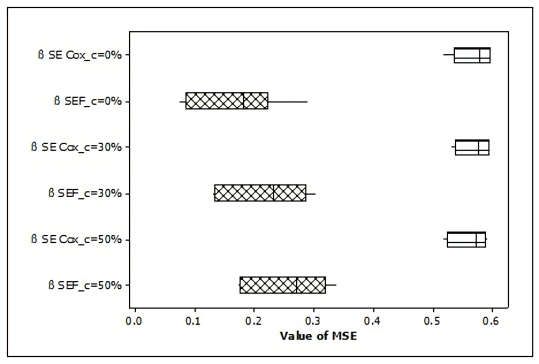
214 Thailand Statistician, 2021; 19(1): 209-228
xij exp( sj )
h* ( i , j )R( i ) 1
sj zij d ( i ) zij v. (13)
v sj k exp( sj )
( i , j )R( i )
Furthermore, to compute variance of ̂ and vˆ, we can generate a second derivative from the
formulation of h* for and v, H (ˆ ) through these following procedures (Dobson 2002)
x x exp ( ) xija exp(ij ) xijp exp (ij )
ija ijp ij
2 h* ( i , j )R( i ) ( i , j )R( i ) ( i , j )R( i )
d(i ) 2 , (14)
a p i exp(ij )
(i , j )R( i ) exp (ij )
( i , j )R
(i )
z z exp( ) zija exp(ij ) ijq x exp( )
2 h* (i , j )R( i ) ija ijq ij
( i , j )R( i ) ( i , j )R( i )
ij
d( i ) 2 , (15)
va q i exp (ij )
(i , j )R( i ) exp(ij )
( i , j )R
(i)
x z exp ( ) xija exp (ij ) ijq z exp( )
2 h* ( i , j )R( i ) ija ijq ij
( i , j )R( i ) ( i , j )R( i )
ij
d(i ) 2 , (16)
a vq i exp(ij )
( i , j )R( i ) exp(ij )
(i , j )R
(i )
z z exp ( ) zija exp(ij ) ijq z exp ( )
2 h* (i , j )R( i ) ija ijq ij
( i , j )R( i ) ( i , j )R( i )
ij
d (i ) 2 . (17)
va vq i exp(ij )
(i , j )R( i ) exp(ij )
(i , j )R
(i)
Thus, according to Hosmer et al. (2008) variance of ̂ and v̂ are
1
2 h*
2 h*
a p
a vq
Var ( ˆ , vˆ) H (ˆ ) 1 . (18)
2 h*
2 h*
v
va vq
a q
To make an estimation of frailty variant ( ), an approach called adjusted profile hierarchical
likelihood can be appropriately employed. (19) below represents its application
1 J
hA* h* log det , (19)
2 2 ˆ , v vˆ
where J = H (ˆ ) .
The maximum likelihood estimation of adjusted profile hierarchical likelihood for can be
hA*
achieved by solving equation 0 using Newton-Raphson method. The first derivative of hA* for
Dewi Juliah Ratnaningsih et al. 215
is expressed in (20) as follows
*
d(i ) m 1 2
h d (i ) log sj sj d (i ) log (2 ) v s ,
i exp( sj ) sj i 2 2 s
(i , j )R( i )
1 J
h*A h* log det ,
2 2 ˆ , v vˆ
d (i ) m 1 2
d (i ) log sj sj d (i ) log (2 ) v s
i exp( sj ) sj i 2 2 s
(i , j )R( i )
1 J
log det ,
2 2
hA* m 1 v2 1 0 0
s2 tr J 1 . (20)
2 2 s 0 1
2
0 0
If J 1 *
Q, then the second derivative of hA for is
0 1
2 hA* m vS2 tr (Q ) tr (Q )
.
2 2 2 s 3 2 2 3
The variance of ˆ are defined in the following equation (Hosmer et al. 2008)
1
2 hA*
Var (ˆ) 2
. (21)
2.3. Simulation design
SEF model is developed to address the presence of unobserved random effect (frailty) in the
previously used model. The steps carried out for the simulation in this paper, which are aimed at
generating time-independent and time-dependent covariates data, data structure and model
assumption, mainly draw on the work by Ratnaningsih et al. (2019). The modelling proposed in this
paper is aimed at extending those steps to include the frailty as the newly added element into the
procedure. The model simulation uses the R program with three packages, namely: survival
(Therneau et al. 2003), frailtyHL (Ha et al. 2019), and Sylvestre et al. (2015).
The random effect (frailty) is assumed to follow N ~ (0, ) distribution across these values:
10, 14, 16 and 20. Model parameters used here are: log (1, 04) and log (0,99), with v 1 for
frailty. The censorings for the model are set out as follows: censoring 0%, C0 ~ Uniform (6,8);
censoring 30%, C30 ~ Uniform (2,5); and censoring 50%, C 50 ~ Uniform (0, 5). The sizes of samples
taken for studies (n) are 100, 500, and 2,000. The simulation is performed with 1,000 iterations.
3. Result and Discussion
3.1. Result of the model simulations
In this section, we describe the merits of the proposed model. The goodness of the model is
indicated by the parameter bias and values of the MSE model. The virtue of the model can be shown216 Thailand Statistician, 2021; 19(1): 209-228
from the results of simulations performed on several combinations of treatment of variance,
censorship, the amount of data, and the number of iterations used. The results of the SEF model
simulation were then compared with the SE Cox model (Ratnaningsih et al. 2019).
Model simulations are applied to 4 types of variance ( ), namely 10, 14, 16, and 20 with 3
types of censoring (0%, 30%, 50%) and 4 sample sizes, namely n 500, 1,000, and 2,000. The
iteration is used 1,000 times. Simulation results for each of the variance, censoring, and sample size
in the biased estimation of model parameters in detail are presented in Table 1.
From Table 1, it can be seen that the estimated bias percentage parameters of the SEF model are
better than the SE Cox model. These are shown from the percentage bias estimation of the model
parameters. In this discussion, a boxplot percentage bias is estimated for model parameters in various
types of censoring (Figures 1-3). From Figure 1, it can be seen that the percentage of the estimated
parameter bias ( ) produced by the SEF model in various types of censoring is smaller than the SE
Cox model. Percentage bias parameter estimation ( ), the SEF model gives a lower percentage than
the SE Cox model. Likewise, with the parameter estimation bias for frailty (v), the SEF model
provides a lower rate of preference than the SE Cox model. Thus, from Table 1 and the three boxplot
drawings, it can be shown that in terms of parameter estimation bias, the SEF model provides the
smallest percentage of bias in various types of censoring.
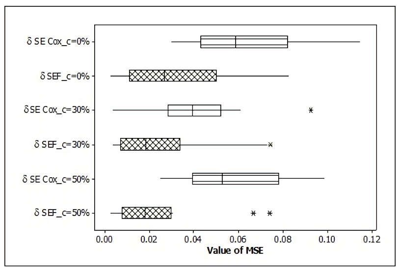
The MSE values generated by both models are presented in Table 1. Graphically the results of
the MSE simulation results on various types of censoring, variance, and sample size are shown in
Figures 4-6. From Table 1 and the three boxplot images presented, it appears that MSE values of
parameters , and v of the SEF model are smaller than the SE Cox model. The MSE value of the
SEF model tends to decrease with an increase in sample size. From the two measures of model
goodness, namely the bias parameters and MSE values, it can be said that the SEF model provides
better modelling results for overcoming the unequal risk model because the existence of frailty and
covariates is time-dependent.
Whether frailty in modelling is influential or not is indicated by the value of the deviation based
on REMPL (Restricted Maximum Partial Likelihood) versus the amount of 2 p , v ( hp ). Then compare
the difference in the variation with the critical value. The different variations of the SEF model are
given in Table 1 (end of the column). From Table 1, the deviation difference column shows that in
general of all the simulations performed, and it appears that frailty has a significant influence on
modelling. This fact is because the deviation value is higher than the critical value. Simulation results
show that the presence of frailty should be considered to form a non-proportional hazard modelling
in survival analysis.
3.2. An Application on real data
SEF modelling presented in this study is intended to be applied to the survival data of the students
of UT. The similar data has previously used by Ratnaningsih et al. (2019) in their study pertaining to
the application of SE Cox model. In the study, the survival-time data constitute the response variable
that is assessed in semester as its measurement unit. The time-independent covariates that are
considered affecting the survival time of the students in their course of study are: educational
background, the study programme of their interest, gender, age, marital status, employement status,
and home area. The time-dependent covariates included in the study are the credit hours completed
by the students, the number of classes they take per semester, and their Grade Average Point (GPA).Dewi Juliah Ratnaningsih et al. 217
Table 1 Result of the simulation models in the various kind of censoring and variance
Note: * is the difference in the SEF model deviation to see whether frailty has an effect or not.
Deviation difference is determined from models with frailty and models without frailty based on
REMPL compared to the critical deviation value of 2.71.218 Thailand Statistician, 2021; 19(1): 209-228
Figure 1 Percentage of bias parameter
Figure 2 Percentage of bias parameter
Figure 3 Percentage of bias parameter Dewi Juliah Ratnaningsih et al. 219
Figure 4 Value of MSE parameter
Figure 5 Value of MSE parameter
Figure 6 Value of MSE parameter 220 Thailand Statistician, 2021; 19(1): 209-228
In applying the model to the real data in their study, Ratnaningsih et al. (2019) do not include
the study programs or majors of study the students are interested in. The reason of the exclusion is
that the courses are assumed as observed random effect. In contrast, in SEF modelling, they belong
to unobserved random effect. SEF model assumes that the involving unobserved random effect
(frailty) is distributed by N (0, 20).
A detailed description of the survival data of the students of UT in their course of study is
presented in Table 2. It is apparent in Table 2 that of the total 4,483 students observed in the present
study, 1,574 (35.11%) are censored and 2,909 (64.89%) are uncensored. The censored students are
those students who are still studying for their degree or who have graduated or who have transferred
to a different major or study programme (active students). The uncensored students are those who no
longer follow the required procedure as a regular student (non-active students), i.e. those students
who fail to register for 4 consecutive semesters (Boton and Gregory 2015).
Table 2 shows the general characteristics of UT students who are non-active. They live in rural
districts, female, between 35 and 45 years old, married, and employed. The data correspond with
Schuemer (1993) that in distance education, the learning process is much more complex because most
of the students who enroll for distance learning courses are of mature age, have a job, and are married.
The similar fact, that is, students who are also employees or professionals will not be able to attend
full-time study (Orr 2000). Age factor contributes significantly to the variations of capability in
undertaking independent learning activities, more specifically in developing a study orientation and
strategies for themselves not only to learn the provided materials but also to gain full comprehension
of the non-conventional academic environment they are dealing with (Kadarko 2000).
Table 2 also informs that the majority of non-active students was the students graduated from
traditional (non-vocational) high schools; have completed 75 credit hours at UT; have GPAs ranging
from 1.00 to 2.00; and have taken 5 to 8 courses for each semester. UT students who came to college
as high school graduates are usually new to independent learning scheme, and their learning
experiences vary. According to Ratnaningsih et al. (2008), several factors that contribute to the
problems UT students have to deal with are: they have not yet fully grasped the way the learning
system at UT works, they are not familiar with independent learning scheme, they have low
motivation to actively engage in the learning process, they don’t have many peers to learn or discuss
with, they have limited access to learning materials, and they have diverse previous educational
experiences. Another factor which also has some bearing on the problem is the lack of discipline or
self-direction on the students’ part.
The results of the SEF model analysis on UT student retention data are presented in Table 3. The
estimated parameters of the random effect unobserved (frailty) in this study are notated by v. The
average of value v produced by the SEF model is 0.01537, and the value of standard error is 0.005834.
The standard error is a measure that illustrates the average distribution of samples over the average
population. A relatively small standard error indicates that the error or average deviation (estimator)
of the population parameter is small. From the estimated size of these parameters, it can be stated that
the SEF model is quite adequate. That is, the SEF model can be used as an alternative modelling of
data hold learning UT students.
Does frailty influence UT student retention learning? This testing criterion uses deviation values
between models without frailty and frailty models. Deviation criteria are calculated based on REMPL
(Restricted Maximum Partial Likelihood) with a value of 2 p , v (hp ). From the results of the case
analysis of UT students, the difference in deviations between models with frailty and without frailty
is 42,369−42,339 = 30. The difference in a deviation between the two models is huge. This showsDewi Juliah Ratnaningsih et al. 221
that frailty has a significant influence on the modelling of UT student retention learning. In the case
of distance education, frailty can be identified with the ID of a student who has an academic record
in online tutorials, learning motivation, learning time management, gaining resource facilities,
ownership of teaching materials, and environmental factors. The frailty aspect for each student is
different. Therefore, it will undoubtedly have a different effect on the success of learning at UT.
Tabel 2 UT students’ characteristics based on the observed covariates
Censored Status
Observed covariates Categorizations Total
Censored Uncensored
Home area Rural district 1,265 2,338 3,603
City 309 571 880
Gender Female 923 1,558 2,481
Male 651 1,351 2,002
Age < 35 years old 87 294 381
35-45 years old 1,049 1,859 2,908
> 45 years old 438 756 1,194
Education High school 813 1,911 2,724
Associate degree 752 959 1,711
Bachelor’s degree 9 39 48
Marital status Unmarried 464 1,081 1,545
Married 1,110 1,828 2,938
Employmnet status Unemployed 58 294 352
Employed 1,516 2,615 4,131
Credit hours completed CH < 75 46 2,197 2,243
75 CH 120 86 402 488
CH> 120 1,442 310 1,752
The number of courses taken each Courses 8 15 372 387
Grade average point 1.00 < GPA 2.00 470 1,962 2,432
2.00 < GPA 3.00 1,074 236 1,310
GPA > 3.00 28 13 41
The analysis shows that statistically significant covariates at alpha 10% are age, GPA, marital
status, number of credits taken, and the number of courses registered per semester. This fact is
consistent with several studies conducted on distance education in several countries such as
Indonesia, Greece, Nigeria, Brazil, New Jersey, Iran, United Kingdom, America, Germany, and
Turkey.
The age of students over 45 years has a significant influence on modelling student learning
retention. This condition can be shown from the p-value less than the alpha level (10%). The
estimated value of the age parameter over 45 years is −0,062. This value means students over the age
of 45 have low learning retention (e0.062 ) or have a risk of 0.940 times compared to the period of
other students. From the analysis of the SEF model, it can be seen that parameter estimates for the
age covariate are positive. This fact shows that students who are younger (lower than 35 years old)
experience high school dropouts. Students who are over 35 years of age tend to have lower learning222 Thailand Statistician, 2021; 19(1): 209-228
resilience than those who have an earlier age. Such conditions are the following studies conducted
by Andriani and Pangaribuan (2006); Kadarko (2000) in Indonesia. Xenos et al. (2002) and
Pierrakeas et al. (2004) in Greece state that there is a correlation between age and dropping out of
college.
Table 3 The parameter estimation results use the SEF model
Observed Covariates Estimate Hazard Ratio Std. Error t-value p-value
Age 35-45 years old 0.063 1.065 0.068 0.931 3.5E-01
Age > 45 years old −0.062 0.940 0.089 −0.697 4.9E-02
Home area (city) 0.016 1.016 0.048 0.327 7.4E-01
Gender (male) 0.029 1.029 0.038 0.754 4.5E-01
1,00 < GPA 2,00 −0.733 0.481 0.048 −15.175 5.2E-52
2,00 < GPA 3,00 0.598 1.818 0.088 −15.950 2.9E-57
GPA > 3,00 0.687 1.988 0.283 −2.431 1.5E-02
Employed −0.017 0.984 0.065 −0.255 8.0E-01
Married −0.078 0.925 0.045 −1.739 7.2E-02
75 CH 120 −1.219 0.295 0.059 −20.723 2.1E-95
CH > 120 −2.848 0.058 0.077 −37.174 1.8E-302
5 Courses 8 0.099 1.104 0.056 1.754 5.9E-02
Courses > 8 −0.497 0.608 0.078 6.373 1.9E-10
Kadarko (2000) revealed that the age factor contributes significantly to the variance in
independent learning abilities, namely the ability to apply orientation and strategy in learning
teaching materials as well as the ability to understand the non-conventional academic environment.
Meanwhile, Pierrakeas et al. (2004) state that younger students (lower than 30 years) tend to drop out
of school. This state is possible because they do not yet have an independent learning experience, and
they tend to underestimate the effort and workload needed for study at the university level.
GPA scores have a significant contribution to student learning retention. Students who have a
GPA between 1.00 and 2.00 tend to have low learning retention. This value is indicated by the
estimated parameter value of −0.733. This condition means that students who have such GPA groups
have a risk of (e0.0733 ) or 0.481 times compared to other students. Meanwhile, students who have a
GPA above 2.00 and even above 3.00 tend to have high learning retention. The risk of surviving is
1.82 and 1.99 times higher than other students. This fact is consistent with studies conducted by
Soeleiman (1991); Ratnaningsih (2008); McCormick and Lucas (2014); Klapproth and Schaltz (2015);
Gaytan (2015); Boton and Gregory (2015). They argued that the GPA was very influential on student
resistance and was a determining factor for the sustainability of studies at the university. Academic
characteristics possessed by students are the determining factors for students dropping out of school.
Employment status and marriage of students also have a significant influence on learning
retention. Students who are working and already married tend to have low learning retention. The
risks are 0.98 and 0.93 times compared to students who are not working and not married. This
condition is in line with the statement of Schuemer (1993) and Rovai (2003). They stated, in general,
the factors that caused dropouts experienced by distance education students included old age, lack of
study time, difficulties in accessing the internet, lack of feedback from tutors, work, family, external
stimuli, and personal financial problems.Dewi Juliah Ratnaningsih et al. 223
The number of credits taken by students also has a significant influence. From the results of the
analysis with the SEF model, students who have earned credits above 75 credits tend to have low
learning retention. But the risk is relatively small at 0.295 and 0.058 compared to other students.
Unlike the case with the number of subjects registered per semester. Students taking 5 to 8 courses
per semester tend to have high learning retention. The risk is 1,104 times compared to students who
earn less than that. However, students who register more than eight subjects tend to have low learning
retention. The risk is 0.608 times compared to students who register less than eight items. This fact
is also consistent with studies conducted by Cambruzzi et al. (2015) in Brazil, which stated that many
students dropped out of college because the credit load did not match the ability of students. For
example, the institution recommends that 12 credits are taken per semester. However, many students
take up to 20 credits because they consider learning with the distance education system easy and can
accelerate their studies. Allen et al. (2016) in the United States revealed that many students took
courses, paid tuition fees, and then dropped out.
3.3. Discussion
From the results of simulations on several treatments, combinations show that the percentage of
parameter bias and MSE model produced by the SEF model is better than the SE Cox model.
Modelling involving frailty factors is very possibly significant so that it can influence modelling on
the actual data. Therefore, through simulations in this study, it can be shown that the SEF model can
be used as alternative modelling involving various covariates (covariates are time-dependent, and
covariates are not time-dependent) and frailty.
In reality, modelling sometimes also has random effects observed. Modelling that involves
random effects and permanent effects is called a mixed effect model. Did not rule out the possibility
of modelling; there are two types of influence so that the development of mixed models can be studied
further. Modelling using a mixed model is possible in a non-comparable risk model. This modelling
is expected to be able to overcome modelling that involves observed random effects, frailty, and other
fixed effects that are thought to influence the model.
The stratified-extended Cox model with frailty (SEF) is a model proposed to address the existence
of two types of covariates (time-dependent covariates and time-dependent covariates) and frailty. Based
on the results of the simulation in various treatment combinations showed that the SEF model was able
to produce a percentage bias of parameters close to the actual value and the MSE value of the model,
which was relatively small compared to the SE Cox model. Based on the two criteria of the model, the
SEF model can be used as an alternative model to overcome the problem of non-proportional hazard in
survival analysis due to the frailty and the two types of covariates mentioned earlier.
The application of the SEF model to the UT student learning resistance data is adequate and can
be used as a satisfying model approach. This reality is because the results of the analysis using the
SEF model are close to the real fact experienced by UT. The presence of frailty in the case of UT
student retention is very significant. Based on the analysis of the SEF covariate model that statistically
significantly affected the retention of Open University students were: educational background, age,
GPA, marital status, number of credits taken, and the number of courses registered per semester. This
condition is also by several other countries that implement distance education systems.
In the UT student data, there is another covariate that is suspected to influence the student's
endurance, namely the study program. This fact is consistent with a study conducted by The 2013
DE Census (CENSO 2014) in Oliveira (2018) that the highest percentage of students dropping out of
school at the Open University of Brazilia depends on the type of study program taken by students. In
modelling, the study program covariate can be assumed to be an observed random effect. Student224 Thailand Statistician, 2021; 19(1): 209-228
retention or course graduation in each study program may vary.
The limitation of SEF modelling is that it does not involve any other random influence other than
frailty. In the case of modelling, there is more than one random influence. The existence of other
random effects in modelling needs treatment, likewise using a mixed effect model. In the case of real
data, another random effect that is thought to be influential in the study program. In the modelling of
mixed effects, the study program can be assumed to be an observed random effect. By entering the
study program into the model, it is expected to produce more valid and accurate modelling. Adequate
and precise modelling can help organizers in determining academic policies that can encourage UT
students to complete their studies on time.
4. Conclusions
Cox proportional hazard (Cox PH) is a frequently used model in survival analysis. This model
assumes that each individual’s hazard rate is proportional to other individuals’ hazard rates with
constant ratio at all times. However, in many cases, an individual’s hazard rate is not always
proportional, and it also fluctuates across certain period of time. This condition is known as non-
proportional hazard.
One of the causes of non-proportional hazard is the presence of unobserved random effect
(frailty) alongside time-dependent and time-independent covariates. The inclusion of frailty in the
process is expected to help generate a valid and accurate model. SEF model is proposed here to
accommodate the presence of two kinds of covariates, time-dependent covariates and time-
independent covariates and frailty. The simulations of different combinations of treatment in this
study show that the parameter bias and MSE generated by SEF model are smaller compared to those
generated by SE Cox model. In conclusion, this model can be considered to be an alternative
statistical modelling to resolve non-proportional hazard issue in survival analysis caused by the
presence of frailty and the two kinds of covariates.
The application of SEF model to the survival data of the students of UT in the course of their
study is suitable, and therefore the model is sufficiently qualified to be an effective approach to the
specified kind of data. Based on the analysis, covariates that significantly affect the survival of the
students of UT in their course of study are: educational background, age, GPA, marital status, the
number of credit hours they completed, and the number of classes they have taken in each semester.
Based on other similar studies, this is a common condition that occurs in other countries where
distance education system is applied by some educational institutions.
Acknowledgments
This research was supported by a grant from the Centre for Research & Community Services of
Universitas Terbuka. The first author thanks the Information and Communication Technology of
Universitas Terbuka for server services during the data simulation process. Also thanks to Lemma
Ferrari Boer for programming research simulation models.
References
Andriani D, Pangaribuan N. Students in open distance education: Theoretical study and applications.
Jakarta: Universitas Terbuka Publishing Center; 2006.
Allen IE, Seaman J, Poulin R, Straut TT. Online report card: Tracking online education in the United
States. Babson Park: Babson Survey Research Group, 2016 [cited 2019 June 10]. Available from:
http://onlinelearningsurvey.com/re-ports/onlinereport-card.
Boton EC, Gregory S. Minimizing attrition in online degree courses. J Educ Online. 2015; 12(1): 62-
90.Dewi Juliah Ratnaningsih et al. 225
Cambruzzi W, Rigo SJ, Barbosa JLV. Dropout prediction and reduction in distance education courses
with the learning analytics multitrail approach. J Univers Comput Sci. 2015; 21(1): 23-47.
Censo EB. Relatório analítico da aprendizagem a distância no Brasil 2013. Associação Brasileira de
Educação a Distância. Curitiba: Ibpex, 2014 [cited 2019 July 28]. Available from
https://www.scielo.br/pdf/ep/v44/en_1517-9702-ep-S1678-4634201708165786.pdf.
Dobson AJ. An Introduction to generalized linear models. New York: Chapman & Hall/CRC; 2002.
Gaytan J. Comparing faculty and student perceptions regarding factors that affect student retention in
online education. Am J Distance Educ. 2015; 29(1): 56-66.
Ha ID, Lee Y, Song JK. Hierarchical likelihood approach for frailty models. Biometrika. 2001; 88(1):
233-243.
Ha ID, Noh M, Kim J, Lee Y. frailtyHL: Frailty Models via Hierarchical Likelihood, R package
version 2.2, 2019 [cited 2019 Oct 16]. Available from: https://cran.r-project.org/web/packages/
frailtyHL/index.html.
Henderson R, Oman JP. Effect of frailty on marginal regression estimates in survival. J R Stat Soc
Series B Stat Methodol. 1999; 61(2): 367-380.
Hosmer D, Lemeshow S, May S. Applied survival analysis. Hoboken: John Wiley & Sons; 2008.
Kadarko W. Understanding students’ learning styles and strategies. J Open Distance Educ. 2000; 3(2):
1-15.
Klapproth F, Schaltz P. Who is retained in school, and when? Survival analysis of predictors of grade
retention in Luxembourgish secondary school. Eur J Psychol Educ. 2015; 30(1): 119-136.
Lee ET, Wang JW. Statistical methods for survival data analysis. Hoboken: John Wiley & Sons;
2003.
McCormick NJ, Lucas MS. Student retention and success: Faculty initiatives at middle Tennessee
State University. JoRRS. 2014; 1(1): 1-12.
Oliveira PR, Oesterreich SA, Almeida VL. School dropout in gradutae distance education: evidence
from a study in the interior of Brazil. Educ Pesqui, 2018; 44, e165786: 1-20.
Orr S. The organizational determinants of success for delivering fee-paying graduate courses.
Int J Educ Manag. 2000; 14(2): 54-61.
Pierrakeas C, Xenos M, Panagiotakopoulos C, Vergidis D. A comparative study of dropout rates and
causes for two different distance education courses. Int Rev Res Open Dis. 2004; 5(2): 1-15.
Ratnaningsih DJ, Saefuddin A, Kurnia A, Mangku IW. Stratified-extended Cox model in survival
modelling of non-proportional hazard. IOP Conference Series: Earth and Environmental Science.
2019; 299(1): 012023.
Ratnaningsih DJ, Saefuddin A, Wijayanto, H. An analysis of drop-out students’ survival in distance
higher education. J Open Distance Educ. 2008; 9(2): 101-110.
Rovai AP. In search of higher persistence rates in distance education online programs. Internet High
Educ. 2003; 6(1): 1-16.
Schuemer R. Some psychological aspects of distance education. Hagen: Institute for Research into
Distance Education; 1993.
Soeleiman N. Continuity of registration and its relation to the examination results. Research Report.
Jakarta: Universitas Terbuka; 1991.
Sylvestre MP, Edens T, MacKenzie T, Abrahamowicz M. PermAlgo: Permutational algorithm to
simulate survival data version 1.1, 2015 [cited 2018 Nov 08]. Available from: https://CRAN.R-
project.org/package=PermAlgo.
Therneau TM, Grambsch PM, Pankratz VS. Penalized survival models and frailty. J Comput Graph
Stat. 2003; 12(1): 156-175.226 Thailand Statistician, 2021; 19(1): 209-228
Vaupel JW, Manton KG, Stallard E. The impact of heterogeneity in individual frailty on the dynamics
of mortality. Demography. 1979; 16(3): 439-454.
Wienke A. Frailty models in survival analysis. New York: Chapman & Hall/CRC; 2011.
Xenos M, Pierrakeas C, Pintelas P. A survey on student dropout rates and dropout causes concerning
the students in the course of informatics of the Hellenic Open University. Comput Educ. 2002;
39(4): 361-377.
Appendix
The script of program simulation for SEF model:
library(frailtyHL)
library(survival)
library(PermAlgo)
set.seed(123)
# Function to generate an individual time-dependent exposure history
# e.g. generate prescriptions of different durations (semester) and doses (sks).
TDhistDewi Juliah Ratnaningsih et al. 227
for (i in 1:length(idx)){
temp228 Thailand Statistician, 2021; 19(1): 209-228
newdataYou can also read