Dynamic causal modelling for fMRI: A two-state model
←
→
Page content transcription
If your browser does not render page correctly, please read the page content below
www.elsevier.com/locate/ynimg
                                                                                                               NeuroImage 39 (2008) 269 – 278

Dynamic causal modelling for fMRI: A two-state model
A.C. Marreiros,⁎ S.J. Kiebel, and K.J. Friston
Wellcome Trust Centre for Neuroimaging, Institute of Neurology, UCL, 12 Queen Square, London WC1N 3BG, UK
Received 14 March 2007; revised 10 July 2007; accepted 6 August 2007
Available online 25 August 2007

Dynamical causal modelling (DCM) for functional magnetic                   hypothesized network, at the neuronal level. The general idea
resonance imaging (fMRI) is a technique to infer directed                  behind DCM is to construct a reasonably realistic neuronal model
connectivity among brain regions. These models distinguish between         of interacting cortical regions with neurophysiologically inspired
a neuronal level, which models neuronal interactions among                 parameters. These parameters are estimated such that the
regions, and an observation level, which models the hemodynamic
                                                                           predicted blood oxygenation level dependent (BOLD) series,
responses each region. The original DCM formulation considered
                                                                           which results from converting the neural dynamics into
only one neuronal state per region. In this work, we adopt a more
plausible and less constrained neuronal model, using two neuronal
                                                                           hemodynamics, correspond as closely as possible to the observed
states (populations) per region. Critically, this gives us an explicit     BOLD series.
model of intrinsic (between-population) connectivity within a                  Standard DCMs for fMRI are based upon a bilinear
region. In addition, by using positivity constraints, the model            approximation to neuronal dynamics with one state per region.
conforms to the organization of real cortical hierarchies, whose           The neuronal dynamics are described by the differential
extrinsic connections are excitatory (glutamatergic). By incorporat-       equations describing the dynamics of a single state that
ing two populations within each region we can model selective              summarizes the neuronal or synaptic activity of each area;
changes in both extrinsic and intrinsic connectivity.                      this activity then induces a hemodynamic response as
    Using synthetic data, we show that the two-state model is
                                                                           described by an extended Balloon model (Buxton et al.,
internal consistent and identifiable. We then apply the model to real
                                                                           1998). Examples of DCM for fMRI can be found in Mechelli
data, explicitly modelling intrinsic connections. Using model
comparison, we found that the two-state model is better than the
                                                                           et al. (2004), Noppeney et al. (2006), Stephan et al. (2005),
single-state model. Furthermore, using the two-state model we find         and Griffiths et al. (2007) (for a review on the conceptual
that it is possible to disambiguate between subtle changes in              basis of DCM and its implementation for functional magnetic
coupling; we were able to show that attentional gain, in the context       resonance imaging data and event-related potentials, see
of visual motion processing, is accounted for sufficiently by an           Stephan et al., 2007).
increased sensitivity of excitatory populations of neurons in V5, to           Dynamical causal modelling differs from established methods
forward afferents from earlier visual areas.                               for estimating effective connectivity from neurophysiological time
© 2007 Elsevier Inc. All rights reserved.                                  series, which include structural equation modelling and models
                                                                           based on multivariate autoregressive processes (Harrison et al.,
Keywords: Functional magnetic resonance imaging; Dynamic causal            2003; McIntosh and Gonzalez-Lima, 1994; Roebroeck et al.,
modelling; Neural mass model                                               2005). In these models, there is no designed perturbation and the
                                                                           inputs are treated as unknown and stochastic. DCM assumes the
                                                                           input to be known, which seems appropriate for designed
                                                                           experiments. Further, DCM is based on a parameterized set of
Introduction                                                               differential equations which can be extended to better describe
                                                                           the system.
   Dynamic causal modelling (DCM) for fMRI is a natural                        Here, we extend the original model to cover two states per
extension of the convolution models used in the standard analysis          region. These states model the activity of inhibitory and
of fMRI (Friston et al., 2003). This extension involves the                excitatory populations. This has a number of key advantages.
explicit modelling of activity within and among regions of a               First, we can relax the shrinkage priors used to enforce stability
                                                                           in single-state DCMs because the interaction of excitatory–
                                                                           inhibitory pairs confers dynamical stability on the system.
 ⁎ Corresponding author. Fax: +44 20 7813 1420.                            Second, we can model both extrinsic and intrinsic connections.
   E-mail address: amarreiros@fil.ion.ucl.ac.uk (A.C. Marreiros).          Third, we can enforce positivity constraints on the extrinsic
   Available online on ScienceDirect (www.sciencedirect.com).              connections (i.e., interregional influences of excitatory popula-
1053-8119/$ - see front matter © 2007 Elsevier Inc. All rights reserved.
doi:10.1016/j.neuroimage.2007.08.019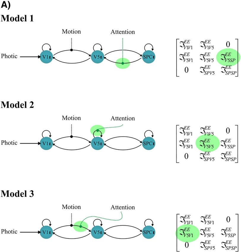
270                                           A.C. Marreiros et al. / NeuroImage 39 (2008) 269–278

tions). Finally, this re-parameterization enables one to model             in a region. Friston et al. (2003) used a bilinear form to describe
context-dependent changes in coupling as a proportional                    their dynamics:

                                                                           z ¼ Fðx; u; hÞcIx þ Cu
increase or decrease in connection strength (cf., the additive
effects used previously; Friston et al., 2003).
     Shrinkage priors are simply priors or constraints on the
parameters that shrink their conditional estimates towards zero
                                                                                       X
(i.e., their prior expectation is zero and the prior variance              I¼Aþ             uj Bð jÞ
determines the degree of shrinkage, in relation to observation                          j
noise). They were employed in early formulations of DCM to
ensure coupling strengths did not attain very high weights,
                                                                                AF A x
which generate exponentially diverging neuronal activity.
However, this motivation for shrinkage priors is rather ad hoc             A¼      ¼    j
and, as we will discuss later, confounds model specification and                Ax   Az u¼0
comparison.
     This paper is structured as follows. In the first section, we
present the two-state DCM, with two states per region. In the                         A2 F   A A x
                                                                           Bð jÞ ¼         ¼
subsequent section, we provide a stability analysis of the two-                      AxAuj Auj Az
state DCM. In the third section, we describe model inversion;
i.e., prior distributions, Bayesian estimation, conditional infer-
ence and model comparison. In Simulations—model compar-                         AF
isons, we compare the single- and two-state DCM using                      C¼      j                                                        ð1Þ
                                                                                Au x¼0
synthetic and real data to establish its face validity. Finally, an
empirical section then demonstrates the use of the two-state                   This model is used to generate neuronal activity; later we will
DCM by looking at attentional modulation of connections during             add hemodynamics and noise to furnish a probabilistic model of
visual motion processing. From these analyses, we conclude that            fMRI measurements. In this model, the state vector x(t) contains
the two-state DCM is a better model for fMRI data than the                 one scalar per region. The changes in neuronal (i.e., synaptic)
single-state DCM.                                                          activity are described by the sum of three effects. First, the matrix
                                                                           A encodes directed connectivity between pairs of regions. The
Theory                                                                     elements of this connectivity matrix are not a function of the
                                                                           input, and can be considered as an endogenous or condition-
Dynamic causal modelling for fMRI—single-state models                      invariant. Second, the elements of B( j) represent the changes of
                                                                           connectivity induced by the inputs, uj. These condition-specific
    In this section we review briefly dynamic causal models of             modulations or bilinear terms B( j) are usually the interesting
fMRI data (Friston et al., 2003). In the next section, we extend           parameters. The endogenous and condition-specific matrices are
this model to accommodate two neuronal sources per region. A               mixed to form the total connectivity or Jacobian matrix I. Third,
dynamic causal model is, like the general linear model, an                 there is a direct exogenous influence of each input uj on each area,
equation which expresses predicted responses in terms of some              encoded by the matrix C. The parameters of this system, at the
parameters and explanatory variables. In our case, the explana-            neuronal level, are given by θn L A, B1,…, BNu, C. At this level,
tory variables are the experimental inputs u, which correspond to          one can specify which connections one wants to include in the
stimulus functions in conventional models. The causal aspect               model. Connections (i.e., elements of the matrices) are removed
comes from control theory, in which the response of causal                 by setting their prior mean and variance to zero. We will illustrate
models can be predicted from the current and past input.                   this later.
Critically, dynamic models do not predict the response per se                  The bilinear form in Eq. (1) can be regarded as an approxi-
but its rate of change. This rate of change can be a complicated           mation to any function, F(z,u,θ), because it is simply a Taylor
nonlinear function of the models unknown parameters and                    expansion around z = 0 and u = 0; retaining only terms that are
known inputs. The form and parameterization of this function is            first-order in the states or input. In this sense, the bilinear model
entailed by the specific DCM used. In fMRI, people generally               can be regarded as a generic approximation, to any [unknown]
use a simple bilinear form with coupling parameter matrices A,             function describing neuronal dynamics, in the vicinity of its
B( j) and C. Critically, the B( j) matrices parameterize interactions      fixed-point; i.e., when the neuronal states are at equilibrium or
between inputs and states; hence, bilinear. The DCMs                       zero.
considered below are multiple-input multiple-output systems                    At the observation level, for each region, the neuronal state
that comprise Nu inputs and Nr outputs with one output per                 forms an input to a hemodynamic model that generates the
region. The Nu inputs correspond to designed causes (e.g.,                 BOLD signal. Region-specific hemodynamics are modelled by
boxcar or impulse stimulus functions used in conventional                  four extra hemodynamic state-variables. The corresponding first-
analyses). Each region produces a measured output that                     order ordinary differential equations are parameterized by five
corresponds to the observed BOLD signal. These time-series                 region-specific parameters, θh (see Friston et al., 2003 for a
would normally be the averages or first eigenvariates of Nr                complete description). Here, we summarize the integration of
selected regions.                                                          the neuronal and hemodynamic states by the generalized
    Interactions among regions are modelled at the neuronal level.         convolution
In single-state models each region has one state variable. This
state is a simple summary of neuronal (i.e., synaptic) activity x(t),      hðtÞ ¼ hðuðtÞ; hÞ:                                               ð2Þ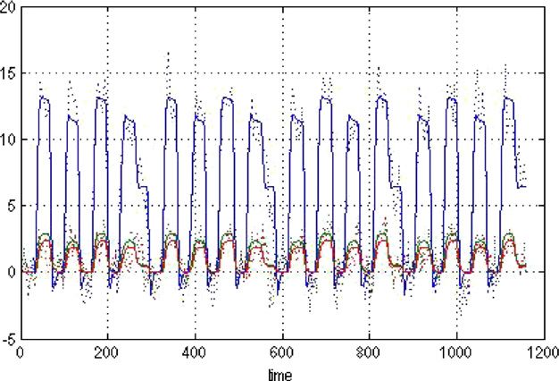
A.C. Marreiros et al. / NeuroImage 39 (2008) 269–278                                                    271

    By integrating the ordinary differential equations of both levels,            excitatory and inhibitory states, {xEi , xIi } of the ith region. These
we can compute the systems predicted hemodynamic response h(t)                    comprise self-connections, E → E, I → I and interstate connections
as a continuous function of time, given the neuronal and                          E → I, I → E. We enforce the connections, E → E, I → E, I → I to be
hemodynamic parameters θ L θn,θh, input u(t), and some initial                    negative (i.e., IEEii ; III ; Iii V0), which means they mediate a
                                                                                                           EI    II

states. Finally, this response is sampled appropriately to form                   dampening effect on population responses. This negativity is
predictions for the BOLD time-series (Kiebel et al., 2007). By                    imposed by using log-normal priors; we use the negative expo-
assuming the observation error ε is Gaussian, we implicitly specify               nential of an underlying coupling parameter with a normal prior
a likelihood model for the ith observation in the time-series                     (see below). Although the excitatory self-connections are negative,
                                         X                                        we do not mean to suggest that there are direct inhibitory connect-
yi ¼ hðti Þ þ ei f pðyjhÞ ¼ NðhðhÞ; ðkÞÞ:                              ð3Þ        ions among excitatory units, rather the multitude of mechanisms
   Where Σ(λ) is the error covariance that is parameterized by an                 that self-organize neuronal activity (e.g., adaptation, gain-control,
unknown hyperparameter. To complete the model specification, we                   refractoriness, polysynaptic input from recurrent axonal collaterals,
need only the priors, p(θ). However, we will first review the                     etc.) will conspire to make the effective self-connection negative.
extension of conventional likelihood models and their implicit re-                The extrinsic connections among areas are assumed to be positive
parameterization.                                                                 (i.e., IEE
                                                                                          ij z0) and are mediated exclusively by coupling among
                                                                                  excitatory populations (cf., glutamatergic projections in the real
                                                                                  brain). In accord with known anatomy, we disallow long-range
Dynamic causal modelling for fMRI—two-state models                                coupling among inhibitory populations.
                                                                                      The two-state DCM has some significant advantages over the
    We now extend the standard DCM above to incorporate two                       standard DCM. First, intrinsic coupling consists of excitatory and
state variables per region. These model the activity of an inhibitory             inhibitory influences, which is biologically more plausible. Also,
and excitatory population respectively. Schematics of the single-                 the interactions between inhibitory and excitatory subpopulations
and two-state models are shown in Fig. 1.                                         confer more stability on the overall system. This means we can
    The Jacobian matrix, I represents the effective connectivity                  relax the shrinkage priors used to enforce stability in single-state
within and between regions. Intrinsic or within-region coupling is                DCMs. Furthermore, we can now enforce positivity constraints on
encoded by the leading diagonal blocks (see Fig. 1), and extrinsic or             the extrinsic connections (i.e., interregional influences among
between-region coupling is encoded by the off-diagonal blocks. Each               excitatory populations) using log-normal priors and scale para-
within-region block has four entries, I••ii ¼ fIEE ii ; Iii ; Iii ; Iii g.
                                                         II    EI    IE
                                                                                  meters as above for the intrinsic connections. This means changes
These correspond to all possible intrinsic connections between the                in connectivity are now expressed as a proportional increase or

Fig. 1. Schematic of the single-state DCM (left) and the current two-state DCM (right). The two-state model has an inhibitory and an excitatory subpopulation.
The positivity constraints are explicitly represented in the two-state connectivity matrix by exponentiation of underlying scale parameters (bottom right).
272 A.C. Marreiros et al. / NeuroImage 39 (2008) 269–278
decrease in connection strength. In what follows, we address each
of these issues, starting with the structural stability of two-state
systems and the implications for priors on their parameters.
Stability and priors
In this section, we will describe a stability analysis of the two-
state system, which informs the specification of the prior
distributions of the parameters. Network models like ours can
display a variety of different behaviours (e.g., Wilson and Cowan,
1973). This is what makes them so useful, but there are
parameterizations which make the system unstable. By this we
mean that the system response increases exponentially. In real
brains, such behaviour is not possible and this domain of parameter
space is highly unlikely to be populated by neuronal systems. The
prior distributions should reflect this by assigning a prior
probability of zero to unstable domains. However, this is not
possible because we have to use normal priors to keep the model
inversion analytically tractable. Instead, we specify priors that are
centered on stable regions of parameter space.
In the original single-state DCM, we had a single state per
region and a self-decay for each state (see Fig. 2). This kind of
system allows for only an exponential decay of activity in each
region, following a perturbation of the state by exogenous input
or incoming connections. For this model, Friston et al. (2003) Fig. 3. Schematic of two-state DCM (one region).
chose shrinkage priors, which were used to initialize the inversion
scheme in a stable regime of parameter space, in which neuronal
activity decayed rapidly. The conditional parameter estimates Friston, 1997). This is a further reason to avoid using shrinkage
were then guaranteed to remain in a stable regime through priors (that preclude systems close to instability). However,
suitable checks during iterative optimization of the parameters. because the bilinear model is linear in its states, its unstable fixed
Two-state models (Fig. 3) can exhibit much richer dynamics points are necessarily associated with exponential growth.
compared to single-state models. Indeed, one can determine
analytically the different kinds of periodic and harmonic oscillatory Priors
network modes these systems exhibit. This is important because it
enables us to establish stability for any prior mean on the We now describe how we specify the priors and enforce
parameters. This entails performing a linear stability analysis by positivity or negativity constraints on the connections. We seek
examining the eigenvalues of the Jacobian, I under the prior priors that are specified easily and are not a function of
expectation of the parameters. The system is asymptotically stable connectivity structure; because this can confound model compar-
if these eigenvalues (cf., Lyapunov spectrum) have only negative ison (Penny et al., 2004). The strategy we use is to determine a
real parts (Dayan and Abbott, 2001). This is the procedure we stable parameterization for a single area, use this for all areas and
adopt below. allow only moderate extrinsic connections. In this way, the system
It should be noted that, in generic coupled nonlinear systems, remains stable for all plausible network structures.
instability of a linearly stable fixed point does not always lead to Priors have a dramatic impact on the landscape of the objective
exponential growth, but may lead to the appearance of a stable function that is optimized: precise prior distributions ensure that
nonlinear regime. In the case of a Hopf bifurcation (as in Wilson the objective function has a global minimum that can be attained
and Cowan, 1973), a limit cycle appears near the unstable fixed robustly. Under Gaussian assumptions, the prior distribution p(θ) is
point, which can model alpha rhythms and other oscillatory defined by its mean and covariance Σ. In our expectation–
phenomena. Indeed, a system close to a linear instability exhibits maximization inversion scheme, the prior expectation is also the
longer and more complex nonlinear transients on perturbation (e.g., starting estimate. If we chose a stable prior, we are guaranteed to
start in a stable domain of parameter space. After this initialization,
the algorithm could, of course, update to an unstable parameter-
ization because we are dealing with a dynamic generative model.
However, these updates will be rejected because they cannot
increase the objective function: in the rare cases an update to an
unstable regime actually occurs (and the objective function
decreases), the algorithm returns to the previous estimate and
halves its step-size, using a Levenberg–Marquardt scheme (Press
et al., 1999). This is repeated iteratively, until the objective
function increases, at which point the update is accepted and the
optimization proceeds. Therefore, it is sufficient to select priors
Fig. 2. Schematic of single-state DCM (one region). whose mean lies in a stable domain of parameter space.A.C. Marreiros et al. / NeuroImage 39 (2008) 269–278 273
Stability is conferred by enforcing connectivity parameters to Table 1
be strictly positive or negative. In particular, the intrinsic, E→E, Log-evidences for three different models using synthetic data generated by
I→I, I→E connections are negative while the E→I and all extrinsic the backward, forward and intrinsic models (see text)
E→E connections are positive. We use Models Synthetic data
Backward Forward Intrinsic
1 0:5
: Backward 523.93 (99.9%) 494.19 (0.0%) 477.50 (0.7%)
0:5 1 Forward 382.07 (0.0%) 538.09 (99.9%) 439.22 (0.0%)
Intrinsic 497.67 (0.0%) 503.55 (0.0%) 482.47 (99.3%)
as the prior mode (most likely a priori) for a single region’s The diagonal values show higher log evidences, which indicate that the two-
Jacobian, where its states, x = [xEi xIi ]T summarize the activity of its state DCM has internal consistency. The percentages correspond to the
constituent excitatory and inhibitory populations. This Jacobian conditional probability of each model, assuming uniform priors over the
has eigenvalues of − 1 ± 0.5i and is guaranteed to be stable. We then three models examined under each data set.
replicate these priors over regions, assuming weak positive
excitatory extrinsic E→E connections, with a prior of 0.5 Hz.
For example, a three-region model, with hierarchical reciprocal the sign of the mode determines whether the connection is positive
extrinsic connections and states, x = [xE1 , xI1, xE2 , xI2, xE3 , xI3]T would or negative. In what follows, we use a prior variance for the
have Jacobian with a prior mode of endogenous and condition-specific coupling parameters, A jkij and
B jk
ij of v = 1/16.
2 3 Re-parameterizing the system in terms of scale-parameters
1 0:5 0:5 0 0 0
6 0:5 1 0 0 0 0 7 entails a new state equation (see Fig. 1), which replaces the
6 7
6 0:5 0 1 0:5 0:5 0 7 Bilinear model in Eq. (1)
A¼6
6 0
7
6 0 0:5 1 0 0 7 7
x ¼ Ix þ Cu
4 0 0 0:5 0 1 0:5 5
0 0 0 0 0:5 1
The eigenvalue spectrum of this Jacobian is show in Fig. 4 (left X
j expðu B
••ðkÞ ••ðkÞ
I••ij ¼ A••ij expðA••ij þ uk Bij Þ ¼ A••ij expðA••ij Þ k ij Þ
panel), along with the associated impulse response functions for
k k
an input to the first subpopulation (right panels); evaluated with
x(t) = exp(μt)x(0). It can be seen for this architecture we expect 2 3 2 E3
neuronal dynamics to play out over a time-scale of about 1 s. Note IEE IEI ::: IEE 0 x1
11 11 1N
6 IIE III11 0 0 7 6 xI 7
that these dynamics are not enforced; they are simply the most 6 11 7 6 17
likely a priori. I¼6 v
6 EE O v 7 6 7
7 x ¼ 6 vE 7 ð4Þ
4I 0 IEE EI 5
INN 4x 5
N1 NN N
0 0 ::: IIE
NN IIINN xIN
Positivity constraints and scale-parameters
To ensure positivity or negativity, we scale these prior modes, μ In this form, it can be seen that condition-specific effects uk act to
with scale-parameters, which have log-normal priors. This is scale the connections by exp(ukB••(k) ••(k) uk
ij ) = exp(Bij ) . When Bij
••(k)
= 0,
••(k)
implemented using underlying coupling parameters with Gaussian this scaling is exp(ukBij ) = 1 and there is no effect of input on the
or normal priors; for example, the extrinsic connections are connection strength. The hemodynamic priors are based on those
parameterized as I••ij ¼ A••ij expðA••ij þ uB••ij Þ, where p(A••
ij ) = N(0,v) used in Friston (2002).
and we have assumed one input. A mildly informative log-normal Having specified the form of the DCM in terms of its likelihood
prior obtains when the prior variance v ≈ 1/16. This allows for a and priors, we can now estimate its unknown parameters, which
scaling around the prior mode, μ•• ij of up to a factor of two, where represent a summary of the coupling among brain regions and how
they change under different experimental conditions.
Bayesian estimation, inference and model comparison
For a given DCM, say model m, parameter estimation corres-
ponds to approximating the moments of the posterior distribution
given by Bayes rule
pðyjh; mÞpðhjmÞ
pðhjy; mÞ ¼ : ð5Þ
pðyjmÞ
The estimation procedure employed in DCM is described in
Friston et al. (2003) and Kiebel et al. (2006). The posterior
moments (conditional mean η and covariance Ω) are updated
Fig. 4. Stability analysis for a two-state DCM (three regions). iteratively using Variational Bayes under a fixed-form Laplace (i.e.,274 A.C. Marreiros et al. / NeuroImage 39 (2008) 269–278
Gaussian) approximation to the conditional density q(θ) = (η,Ω). comparison rests on the likelihood ratio of the evidence for two
This is formally equivalent to expectation–maximization (EM) that models. This ratio is the Bayes factor Bij. For models i and j
employs a local linear approximation of Eq. (2) and Eq. (4) about
the current conditional expectation. ln Bij ¼ lnpð yjm ¼ iÞ lnpð yjm ¼ jÞ: ð8Þ
Often, one wants to compare different models for a given data
Conventionally, strong evidence in favour of one model
set. We use Bayesian model comparison, using the model evidence
requires the difference in log-evidence to be about three or more
(Penny et al., 2004), which is
(Penny et al., 2004). Under the assumption that all models are
Z equally likely a priori, the marginal densities p(y|m) can be
pðyjmÞ ¼ pðyjh; mÞpðhjmÞdh: ð6Þ converted into the probability of the model given the data p(m|y)
(by normalizing so that they sum to one over models). We will
Note that the model evidence is simply the normalization use this probability to quantify model comparisons below (see
constant in Eq. (5). The evidence can be decomposed into two Tables).
components: an accuracy term, which quantifies the data fit, and a
complexity term, which penalizes models with redundant para- Simulations—model comparisons
meters. In the following, we approximate the model evidence for
model m, under the Laplace approximation, with Here we establish the face validity of the DCM described in
the previous section. This was addressed by integrating DCMs
lnpð yjmÞclnpð yjk; mÞ: ð7Þ with known parameters, adding observation noise to simulate
responses and inverting the models. Crucially, we used different
This is simply the maximum value of the objective function models during both generation and inversion and evaluated all
attained by EM. The most likely model is the one with the largest combinations to ensure that model section identified the correct
log-evidence. This enables Bayesian model selection. Model model.
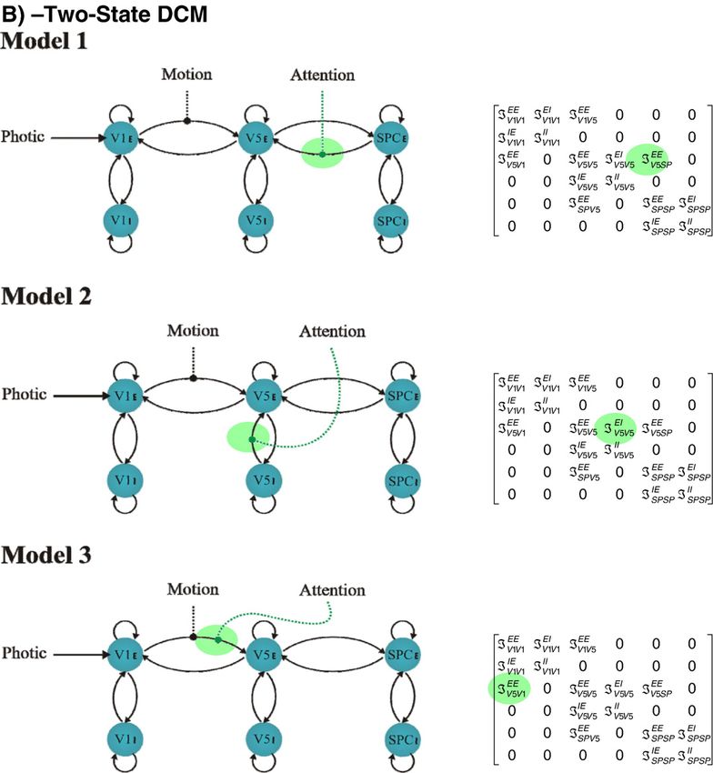
Fig. 5. In all models photic stimulation enters V1 and the motion variable modulates the connection from V1 to V5. Models 1, 2 and 3 all assume reciprocally and
hierarchically organized connections. They differ in how attention modulates the influences on V5; Model 1 assumes modulation of the backward extrinsic
connection, Model 2 assumes modulation of intrinsic connections in V5 and Model 3 assumes modulation of the forward connection. A: single-state DCMs. B:
two-state DCMs.A.C. Marreiros et al. / NeuroImage 39 (2008) 269–278 275
Fig. 5 (continued).
The DCMs used the posterior or conditional means from three
different models estimated using real data (see next section). We
added random noise such that the final data had a signal-to-noise
ratio of three, which corresponds to typical DCM data1. We created
three different synthetic data sets corresponding to a forward,
backward and intrinsic model of attentional modulation of
connections in the visual processing stream. We used a hierarchal
three-region model where stimulus-bound visual input entered at
the first or lowest region. In the forward model, attention increased
coupling in the extrinsic forward connection to the middle region;
in the backward model it changed backward influences on the
middle region and in the intrinsic model attention changed the
intrinsic I→E connection. In all models, attention increased the
sensitivity of the same excitatory population to different sorts of
afferents.
1
Note that a DCM time-series of a single region is the first eigenvariate Fig. 6. Plot of the DCM fit to visual attention fMRI data, using the two-state
of a cluster of voxels and is relatively denoised. Model 3. Solid: Prediction; Dotted: Data.276 A.C. Marreiros et al. / NeuroImage 39 (2008) 269–278
Fig. 7. Results of the Bayesian model comparisons among DCMs for single-state (left) and two-state (right) formulations. The graphs show the log-evidences for
each model: Model 3 (modulation of the forward connections by attention) is superior to the other two models. The two-state model log-evidences are better than
any single-state model (note the difference in scale).
We then used the three models to fit each of these three Model 2 assumed that attention modulates the intrinsic connection
synthetic data sets, giving nine model inversions. Table 1 presents in V5 and Model 3 assumed attention modulates the forward
the log-evidences for each inversion. The highest evidences were connection from V1 to V5. All models assumed that the effect of
obtained for models that were used to generate the synthetic data: motion was to modulate the connection from V1 to V5. In Fig. 5
these correspond to the diagonal entries. These results show that we show each of these three variants for the single- and two-state
model comparison can identify reliably the correct model, among DCM.
competing and subtly different two-state models. We inverted all models using the variational EM scheme above
and compared all six DCMs using Bayesian model comparison. As
Empirical analyses—model comparisons a representative example of the accuracy of the DCM predictions,
we show the predicted and observed BOLD series for Model 3
In this section we ask whether the two-state extension described (two-state) in Fig. 6. The results of the Bayesian model comparison
in this paper is warranted, in terms of providing a better are shown in Fig. 7, in terms of the log-evidences (in relation to a
explanation of real data. This was addressed by inverting the baseline model with no attentional modulation). These results show
single- and two-state models using the same empirical data. These two things. First, both models find strong evidence in favour of
data have been used previously to validate DCM and are available Model 3, i.e., attention modulates the forward connection from V1
from http://www.fil.ion.ucl.ac.uk/spm. We analyzed data from a to V5. Second, there is strong evidence that the two-state Models 2
study of attentional modulation during visual motion processing and 3 are better than any single-state model. The respective log-
(Büchel and Friston, 1997). The experimental manipulations were evidences for this Bayesian model comparison among DCMs
encoded as three exogenous inputs: A ‘photic stimulation’ input (Büchel and Friston data) are shown in Table 2. Again, the table
indicated when dots were presented on a screen, a ‘motion’ shows that the forward model is the best model, among either the
variable indicated that the dots were moving and the ‘attention’ single- or two-state DCMs. Moreover, there is very strong evidence
variable indicated that the subject was attending to possible in favour of the two-state model over the single-state model,
velocity changes. The activity was modelled in three regions V1, because the differences in log-evidences are all greater than five.
V5 and superior parietal cortex (SPC). For reference; the log-evidence for the baseline model with no
We compared the single- and two-state DCM over the attentional modulation was − 1649.9.
following three model variants. Model 1 assumed that attention These results represent an inference on model space. To illus-
modulates the backward extrinsic connection from SPC to V5. trate inference on parameter space, Fig. 8 shows the conditional
Table 2
This table shows the log-evidences for the two models, single and two-state DCMs, plotted in the previous figure
Backward Forward Intrinsic
Single-state DCM −1649.38 (0.00%) − 1647.36 (0.00%) − 1648.60 (0.00%)
Two-state DCM −1629.20 (1.08%) − 1624.80 (88.12%) − 1626.90 (10.79%)
Difference in log-evidence 20.180 22.560 21.700
Forward modulation is the best for both models. We can also see that that there is very strong evidence in favour of the two-state model over the single-state
model. The percentages in bold correspond to the conditional probability of each model, given the data and assuming uniform priors over the six models
examined.A.C. Marreiros et al. / NeuroImage 39 (2008) 269–278 277
fMRI data: currently, we model excitatory (glutamatergic) and
inhibitory (GABAergic) connections. As a natural extension we
can include further states per region, accounting for other
neurotransmitter effects. Important examples here would be
adaptation phenomena and activity-dependent effects of the sort
mediated by NMDA receptors. This is interesting because NMDA
receptors are thought to be targeted preferentially by backward
connections. This could be tested empirically using a suitable
multistate DCM based on an explicit neural mass model.
Another important point is that the hemodynamics in the
current DCM are a function of the excitatory states only. The
contributions to the BOLD signal from the inhibitory states are
expressed indirectly, through dynamic interactions between the two
states, at the neuronal level. One possible extension would be to
model directly separate contributions of these two states, at the
hemodynamic level. Hypotheses about the influence of excitatory
and inhibitory populations on the BOLD signal could then be
tested using model comparison.
Another extension is to generalize the interactions between the
Fig. 8. Posterior probability density functions for the Gaussian parameter,
BEE(3) associated with attentional modulation of the forward connection in two subpopulations, i.e., to use nonlinear functions of the states in
ij
the best model. There is an 88% confidence that this gain is greater than one the DCM. Currently, this is purely linear in the states, but one
(area under the Gaussian to the right of the dashed line). The dashed line could use sigmoidal functions. This would take our model into the
indicates BEE(3)
ij = 0⇒exp(BEE(3)
ij ) = 1. class described by Wilson and Cowan (1973). In this fashion, one
can construct more biologically constrained response functions and
density of the parameters representing attentional gain of the bring DCMs for fMRI closer to those being developed for EEG
forward connection in the best model. We show this conditional and MEG. Again, the question of whether fMRI data can inform
density on the Gaussian parameter, BEE(3)ij (with an implicit gain or such neural mass models can be answered simply by model
scale-parameter exp(BEE(3)
ij )) associated with attention (i.e., when comparison. As noted above, the bilinear approximation used in
u3 = 1). It can be seen that we can be 88% confident that this gain is the original formulation of DCM for fMRI represents a global
greater than one. linearization over the whole of state-space; the current extension
uses the same bilinear approximation in the states (although it is
nonlinear in the parameters). Further refinements to the model,
Discussion such as applying a sigmoid nonlinearity (cf., Wilson and Cowan,
1973) would give a state equation that is nonlinear in the states. In
In this paper, we have described a new DCM for fMRI, which this instance, we can adopt a local linearization, when integrating
has two states per region instead of one. With the two-state DCM, the system to generate predictions. In fact, our inversion scheme
it is possible to relax shrinkage priors used to guarantee stability in already uses a local linearization because the hemodynamic part of
single-state DCMs. Moreover, we can model both extrinsic and DCM for fMRI is nonlinear in the hemodynamic states (Friston,
intrinsic connections, as well as enforce positivity constraints on 2002). However, this approach does not account for noise on the
the extrinsic connections. states (i.e., random fluctuations in neuronal activity). There has
Using synthetic data, we have shown that the two-state model already been much progress in the solution of stochastic
has internal consistency. We have also applied the model to real differential equations entailed by stochastic DCMs, particularly
data, explicitly modelling intrinsic connections. Using model in the context of neural mass models (see Valdes et al., 1999;
comparison, we found that the two-state model is better than the Sotero et al., 2007).
single-state model and that it is possible to disambiguate between Finally, in the next development of DCM for fMRI, we will
subtle changes in coupling; in the example presented here, we were evaluate DCMs based on density-dynamics. Current DCMs
able to show that attentional gain, in the context of visual motion consider only the mean neuronal state for each population. In
processing, is accounted for sufficiently by an increased sensitivity future work we will replace the implicit neural mass model with
of excitatory populations of neurons in V5 to forward afferents full-density dynamics, using the Fokker–Planck formalism. This
from earlier visual areas. would allow one to model the interactions between mean neuronal
These results suggest that the parameterization of the standard states (e.g., firing rates) and their dispersion or variance over each
single-state DCM is possibly too constrained. With a two-state population of neurons modelled.
model, the data can be explained by richer dynamics at the
neuronal level. This might be seen as surprising because it Conclusion
generally is thought that the hemodynamic response function
removes a lot of information and a reconstruction of neuronal Our results indicate that one can estimate intrinsic connection
processes is not possible. However, our results challenge this strengths within network models using fMRI. Using real data, we
assumption, i.e., DCMs with richer dynamics (and more find that a two-state DCM is better than the conventional single-
parameters) are clearly supported by the data. state DCM. The present study demonstrates the potential of
In the following, we discuss some potential extensions to adopting generative models for fMRI time-series that are informed
current DCMs that may allow useful questions to be addressed to by anatomical and physiological principles.278 A.C. Marreiros et al. / NeuroImage 39 (2008) 269–278
Acknowledgments McIntosh, A.R., Gonzalez-Lima, F., 1994. Structural equation modeling and
its application to network analysis in functional brain imaging. Hum.
This work was supported by the Portuguese Foundation for Brain Mapp. 2, 2–22.
Mechelli, A., Price, C.J., Friston, K.J., Ishai, A., 2004. Where bottom-up
Science and Technology and the Wellcome Trust.
meets top-down: neuronal interactions during perception and imagery.
Cereb. Cortex 14, 1256–1265.
References Noppeney, U., Price, C.J., Penny, W.D., Friston, K.J., 2006. Two distinct
neural mechanisms for category-selective responses. Cereb. Cortex 16
Büchel, C., Friston, K.J., 1997. Modulation of connectivity in visual (3), 437–445.
pathways by attention: cortical interactions evaluated with structural Penny, W.D., Stephan, K.E., Mechelli, A., Friston, K.J., 2004. Comparing
equation modelling and fMRI. Cereb. Cortex 7, 768–778. dynamic causal models. NeuroImage 22 (3), 1157–1172.
Buxton, R.B., Wong, E.C., Frank, L.R., 1998. Dynamics of blood flow and Press, W.H., Flannery, B.P., Teukolsky, S.A., Vetterling, W.T., 1999.
oxygenation changes during brain activation: the Balloon model. MRM Numerical Recipes in C: The Art of Scientific Computing. Cambridge
39, 855–864. University Press.
Dayan, P., Abbott, L.F., 2001. Theoretical Neuroscience: Computational and Roebroeck, A., Formisano, E., Goebel, R., 2005. Mapping directed
Mathematical Modeling of Neural Systems. MIT Press. influence over the brain using Granger causality and fMRI. NeuroImage
Friston, K.J., 1997. Another neural code? NeuroImage 5 (3), 213–220. 25 (1), 230–242.
Friston, K.J., 2002. Bayesian estimation of dynamical systems: an Stephan, K.E., Penny, W.D., Marshall, J.C., Fink, G.R., Friston, K.J., 2005.
application to fMRI. NeuroImage 16 (2), 513–530. Investigating the functional role of callosal connections with dynamic
Friston, K.J., Harrison, L., Penny, W., 2003. Dynamic causal modelling. causal models. Ann. N. Y. Acad. Sci. 1064, 16–36.
NeuroImage 19, 1273–1302. Stephan, K.E., Harrison, L.M., Kiebel, S.J., David, O., Penny, W.D., Friston,
Griffiths, T.D., Kumar, S., Warren, J.D., Stewart, L., Stephan, K.E., Friston, K.J., 2007. Dynamic causal models of neural system dynamics: current
K.J., 2007. Approaches to the cortical analysis of auditory objects. Hear. state and future extensions. J. Biosci. 32, 129–144.
Res., doi:10.1016/j.heares.2007.01.010. Sotero, R.C., Trujillo-Barreto, N.J., Iturria-Medina, Y., Carbonell, F.,
Harrison, L.M., Penny, W., Friston, K.J., 2003. Multivariate autoregressive Jimenez, J.C., 2007. Realistically coupled neural mass models can
modelling of fMRI time series. NeuroImage 19 (4), 1477–1491. generate EEG rhythms. Neural Comput. 19 (2), 478–512.
Kiebel, S.J., David, O., Friston, K.J., 2006. Dynamic causal modelling of Valdes, P.A., Jimenez, J.C., Riera, J., Biscay, R., Ozaki, T., 1999. Nonlinear
evoked responses in EEG/MEG with lead field parameterization. EEG analysis based on a neural mass model. Biol. Cybern. 81 (5–6),
NeuroImage 30, 1273–1284. 415–424.
Kiebel, S.J., Kloppel, S., Weiskopf, N., Friston, K.J., 2007. Dynamic causal Wilson, H.R., Cowan, J.D., 1973. A mathematical theory of the functional
modeling: a generative model of slice timing in fMRI. NeuroImage 34 dynamics of cortical and thalamic nervous tissue. Kybernetik 13,
(4), 1487–1496 (Feb 15). 55–80.You can also read