Data suggest COVID 19 affected numbers greatly exceeded detected numbers, in four European countries, as per a delayed SEIQR model - Nature
←
→
Page content transcription
If your browser does not render page correctly, please read the page content below
www.nature.com/scientificreports
OPEN Data suggest COVID‑19
affected numbers greatly
exceeded detected numbers,
in four European countries,
as per a delayed SEIQR model
Sankalp Tiwari1, C. P. Vyasarayani 2*
& Anindya Chatterjee1
People in many countries are now infected with COVID-19. By now, it is clear that the number of
people infected is much greater than the number of reported cases. To estimate the infected but
undetected/unreported cases using a mathematical model, we can use a parameter called the
probability of quarantining an infected individual. This parameter exists in the time-delayed SEIQR
model (Scientific Reports, article number: 3505). Here, two limiting cases of a network of such models
are used to estimate the undetected population. The first limit corresponds to the network collapsing
onto a single node and is referred to as the mean-β model. In the second case, the number of nodes
in the network is infinite and results in a continuum model wherein the infectivity is statistically
distributed. We use a generalized Pareto distribution to model the infectivity. This distribution has
a fat tail and models the presence of super-spreaders that contribute to the disease progression.
While both models capture the detected numbers well, the predictions of affected numbers from the
continuum model are more realistic. Our results suggest that affected people outnumber detected
people by one to two orders of magnitude in Spain, the UK, Italy, and Germany. Our results are
consistent with corresponding trends obtained from published serological studies in Spain, the UK and
Italy. The match with limited studies in Germany is poor, possibly because Germany’s partial lockdown
approach requires different modeling.
For different countries around the world, several r esearchers1–7 have concluded that the number of people actu-
ally infected, or affected, by COVID-19 is far greater than the number of cases actually reported, or detected
officially. Recent serological surveys for COVID-19 also indicate that the infected people outnumber detected
people by about 12 times in Spain8 and 6 to 24 times in the USA9. Other serological surveys suggest that about
18% of people in L ondon10 and 23% of the people in New D elhi11 were already infected by mid-April and early
July, respectively, far outnumbering the reported cases.
In other words, affected numbers seem to greatly exceed detected numbers. To what extent can this difference
be anticipated from pure data fitting of detected people, simple parameter estimation, and simple epidemiological
models? That is the question we take up in this paper.
We fit two time-delayed SEIQR (Susceptible, Exposed, Infected, Quarantined or Isolated, Recovered/Removed)
models to the numbers of reported cases against time, for four European countries. These countries were chosen
because they are not extremely large and diverse (e.g., the USA and India), they have cultural differences amongst
them, and yet they are geographically close to each other. In other words, they are different from each other but
not vastly different. Note that these four countries have largely Caucasian populations, have comparable land
areas, have a small latitude and longitude range, allowed free travel between countries prior to the pandemic,
and have similar development indices, among other similarities. Yet, there are differences in language, culture,
and diet. Moreover, their lockdown policies have been similar in some ways, yet different in others. For instance,
Italy, the UK and Spain opted for a full lockdown, while Germany opted for a partial lockdown12.
1
Mechanical Engineering, Indian Institute of Technology Kanpur, Kanpur 208016, India. 2Mechanical and Aerospace
Engineering, Indian Institute of Technology Hyderabad, Sangareddy 502285, India. *email: vcprakash@
mae.iith.ac.in
Scientific Reports | (2021) 11:8106 | https://doi.org/10.1038/s41598-021-87630-z 1
Vol.:(0123456789)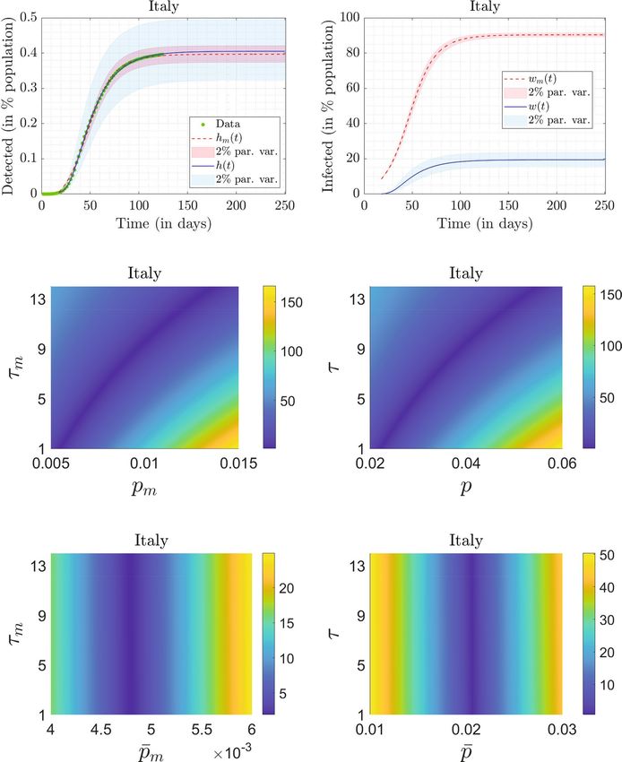
www.nature.com/scientificreports/
These models are obtained by considering two limiting cases of a time-delayed network SEIQR model moti-
vated by the model of Young et al.13–15. In the network model, the whole population is divided into N sub-
populations based on their net infectivity (β ) values, and each node represents a sub-population or group. In
the first limiting case that we adopt, which is the same as a mean-β model15, the entire network14 is collapsed
into a single node ( N = 1). This model was originally proposed by Young et al.13, and for a fast pandemic some
simplifications and approximations are possible15. In the second limiting case14, which is a continuum model, we
take N → ∞. Here, the infectivity is treated as a continuously distributed parameter in the population. Note that
these models are not network models themselves, but are the extreme limits of an underlying network model.
Please see the books by Barrat et al.16 and Barabási17 for more details on network models.
For Italy, Germany, the UK, and Spain, we fit these two models to the data reported under the heading ‘total
cases’ on the Worldometer website18. We consider the data from February 15–June 18 for fitting (125 days).
Beyond mid-June, all the countries seemed to be experiencing a second wave of COVID-19 after relaxing social
distancing norms, or perhaps due to increased testing rates. Therefore, the constancy of model parameters beyond
mid-June may not be a reasonable assumption.
Both these models include a parameter called the probability of detecting an infected individual. This param-
eter, upon fitting from detected population data, allows us to indirectly estimate the affected but undetected popu-
lation. We will find that the continuum model fits the data better than the mean-β model. The continuum model
predicts that the affected people outnumber the detected people by 8, 22, 48, and 130 times in Spain, the UK,
Italy, and Germany, respectively. However, it is emphasized that only the officially detected numbers are used for
data fitting. The continuum model also indirectly suggests the presence of ‘super-spreaders’ (or ‘super-spreading
events’) in all the countries, in the form of a fat tail in the distribution of the infectivity β in the population.
We point out the differences between our network model and complex network models. In our model, each
node k represents a portion of the susceptible population with infectivity√ √βk . Further, each node k is connected
to every other node r = 1, 2, . . . , N with coupling coefficient βkr = βk βr . In complex network models, these
coupling coefficients are referred to as weights19. In the continuum limit of our model, when N → ∞, the initial
infectivity corresponding to each node (population group) is assumed to follow a Pareto distribution φ(β).
In complex scale-free networks, the number of nodes are large but finite. Usually, their degree distribution
follows a power-law20. Sometimes, the distribution of weights of the network may also have a fat t ail19. Super
spreading events are known to occur in complex networks20. For example, in the work of Saumell-Mendiola
et al.21, it was showed that by connecting two complex scale-free networks by a small number of connections
(super spreaders), it is possible to achieve endemic equilibrium. Without this small number of connections, the
disease did not progress in either of their networks. Finally, we emphasize that our network model’s continuum
limit allowed us to make certain mathematical simplifications14, which led to a collapse in the dimensionality
of the system.
The rest of this paper is organized as follows. In “SEIQR models” section, we briefly discuss the two models
(mean-β and continuum) used in this work. “The case of Italy” section, we present and discuss in detail the results
of the optimization calculations (i.e., parameter fitting) for Italy. In “The cases of Germany, UK, and Spain” sec-
tion, we present the results for the remaining three countries: Germany, the UK and Spain. In “Conclusions”
section, we present our conclusions. In the supplementary material for this paper, we present a detailed study
investigating other infectivity distributions in the continuum model, and some sensitivity analysis results.
SEIQR models
A detailed description of the mean-β model15 ( N = 1) and the continuum m odel14 ( N → ∞) can be found in
the literature. In this section, we describe them briefly for clarity and completeness.
Mean‑β model. The mean-β model15 can be derived from the five state SEIQR model of Young et al.13 by
assuming no loss of immunity after recovery. This assumption is valid for a fast pandemic like COVID-19. In the
mean-β model, exposed ( Em), quarantined (Qm), and recovered (Rm) states becomes slave variables of suscepti-
ble (Sm) and infected ( Im) states whose dynamics are governed by the following DDEs:
Ṡm (t) = −βm Sm (t)Im (t), (1)
İm (t) = βm Sm (t − σm )Im (t − σm ) − pm e−γm τm βm Sm (t − σm − τm )Im (t − σm − τm ) − γm Im (t). (2)
The parameters pm, γm, τm, βm, and σm are described in Table 1. The subscript m in all the quantities serves to
distinguish them from those used in the continuum model ( N → ∞). By defining
t
V (t) = Im (η) dη, (3)
−∞
and integrating Eq. (1), we get
Sm (t) = e−βm V (t) , (4)
where we have imposed the initial condition Sm (−∞) = 1. Inserting Eqs. (3) and (4) into (2), we obtain
V̈ (t) = βm e−βm V (t−σm ) V̇ (t − σm ) − pm e−γm τm βm e−βm V (t−σm −τm ) V̇ (t − σm − τm ) − γm V̇ (t). (5)
Integrating both sides of the above equation and by defining
Scientific Reports | (2021) 11:8106 | https://doi.org/10.1038/s41598-021-87630-z 2
Vol:.(1234567890)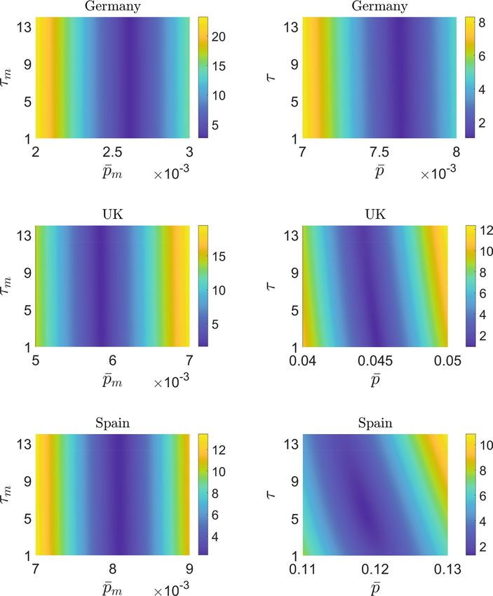
www.nature.com/scientificreports/
S. no. Parameter Description Ranges Specified/estimated
1 σm Asymptomatic and non-infectious period σm = 3 Specified
2 τm Infectious but asymptomatic period 1 ≤ τm ≤ 14 Estimated
3 γm Self-recovery rate γm = 0.07 Specified
4 pm Probability of quarantining symptomatics 0 ≤ pm ≤ 1 Estimated
5 βm Infectivity constant βm > 0 Estimated
6 V0 History of V for DDE V0 > 0 Estimated
Table 1. Parameters used in the mean-β model.
S. No. Parameter Description Ranges Specified/estimated
1 σ Asymptomatic and non-infectious period σ =3 Specified
2 τ Infectious but asymptomatic period 1 ≤ τ ≤ 14 Estimated
3 γ Self-recovery rate γ = 0.07 Specified
4 p Probability of quarantining symptomatics 0≤p≤1 Estimated
5 a Parameter in ψ(u) a>0 Estimated
6 m Denominator exponent in ψ(u) m>2 Estimated
7 f0 History of f for DDE f0 > 0 Estimated
Table 2. Parameters used in the continuum model.
p̄m = pm e−γm τm , (6)
we obtain
V̇ (t) = p̄m e−βm V (t−σm −τm ) − e−βm V (t−σm ) − γm V (t) + 1 − p̄m . (7)
The complete dynamics of the pandemic in the mean-β can be captured by the first-order nonlinear DDE given
by Eq. (7). The percentage of population detected as having contracted the disease is given by
t
hm (t) = 100p̄m βm e−βm V (t−σm −τm ) V̇ (t − σm − τm ) dt, (8)
−∞
and the percentage of population infected (detected plus undetected) till time t is
wm (t) = 100(1 − e−βm V (t) ), (9)
The biological parameters σm and γm are fixed at values reported in the COVID-19 l iterature22–24.
Continuum model. The other limit of the network model14 is for the case of N → ∞, which implies that
the infectivity (β) is now distributed continuously over the population. The governing differential equations for
the states S and I in this case are as follows:
∞
Ṡ(β, t) = − βS(β, t) ξ I(ξ , t) dξ , (10)
0
∞
∞
ξ I(ξ , t − σ ) dξ − pe−γ τ
İ(β, t) = βS(β, t − σ ) βS(β, t − σ − τ ) ξ I(ξ , t − σ − τ ) dξ − γ I(β, t),
0 0
(11)
where p, γ , τ , and σ are described in Table 2. It has been s hown14 that S(β, t) admits a solution of the form:
√
S(β, t) = φ(β)e−f (t) β
. (12)
Therefore, if the initial distribution of infectivity in the population, φ(β), is specified, the subsequent variation
of S is simply through f(t). Using algebraic manipulations, it has been shown that f(t) satisfies the following
non-linear DDE14 :
f˙ (t) = −G(f (t − σ )) + pe−γ τ G(f (t − σ − τ )) − γ f (t) + C0 , (13)
where
Scientific Reports | (2021) 11:8106 | https://doi.org/10.1038/s41598-021-87630-z 3
Vol.:(0123456789)www.nature.com/scientificreports/
∞
√
G(f (t)) = βφ(β)e−f (t) β
dβ, (14)
0
and
∞
C0 = (1 − pe−γ τ ) βφ(β) dβ.
0
√
It is useful to introduce a new random variable u = β with probability density function ψ(u), such that
ψ(u) = 2uφ(u2 ). Then,
∞
G(f (t)) = uψ(u)e−f (t)u du (15)
0
and
∞
C0 = (1 − pe−γ τ ) uψ(u) du. (16)
0
The quantities corresponding to Eqs. (8) and (9) now are
t
h(t) = 100pe−γ τ f˙ (t̄ − σ − τ )G(f (t̄ − σ − τ )) d t̄ (17)
−∞
and
∞
∞
w(t) = 100 1 − S(β, t) dβ = 100 1 − ψ(u)e−f (t)u du , (18)
0 0
In the present work, we assume ψ(u) to be of the form
(m − 1)am−1
ψ(u) = , u > 0,
(a + u)m
istribution25. This means that
which is a generalized Pareto d
(m − 1)am−1
φ(β) = √ √ , β > 0. (19)
2 β(a + β)m
Note that
∞ ∞
φ(β) dβ = ψ(u) du = 1.
0 0
In the supplementary material, we have presented a detailed study investigating other distributions for ψ(u).
That discussion supports our choice of the generalized Pareto distribution.
A summary of the parameters used in the continuum model is presented in Table 2. Note that m > 2 ensures
that u has a finite mean. If m > 3, then u has finite variance as well.
The fitting error. In the mean-β model, for a given set of parameter values, we compute hm (t) and fit it
with the data for the total number of detected cases as reported on the Worldometer website18. This is done by
minimizing the fitting error
||hm − data ||2
E0m = × 100. (20)
|| data ||2
We see from Table 1 that there are four parameters to be identified in the mean-β model. The fitting error for
the continuum model is defined as
||h − data ||2
E0 = × 100. (21)
|| data ||2
We see from Table 2 that there are five parameters to be identified in the continuum model.
Sensitivity analysis. To test the sensitivity of both the models to both fixed and fitted parameters, the
parameters are varied by ±2% around the values corresponding to the optimum fit. We generate 10,000 param-
eter sets using the Latin Hypercube sampling command lhsdesign in MATLAB26. Including the two exter-
nally specified parameters σ and γ , the hypercube is six dimensional in the mean-β model, and seven dimen-
sional in the continuum model. The fits corresponding to these samples are plotted using bands of lighter shades
around the optimum fits plotted in darker shades. Results will be presented in "The case of Italy" and "Results for
the mean-β model" sections below.
Scientific Reports | (2021) 11:8106 | https://doi.org/10.1038/s41598-021-87630-z 4
Vol:.(1234567890)www.nature.com/scientificreports/
Country βm pm τm p̄m = pm e −γm τm V0 E0m A/D R0
Italy 0.1825 0.0112 12.1157 0.0048 0.4861 1.8770 228 2.5953
Germany 0.2097 0.0069 13.8161 0.0026 0.5211 2.6831 426 2.9882
UK 0.1636 0.0137 12.2077 0.0058 0.4773 1.6211 185 2.3240
Spain 0.1785 0.0194 12.5517 0.0081 0.7386 2.2480 142 2.5296
Table 3. Parameter sets from mean-β model yielding the lowest E0m, and subsidiary quantities.
We also study the sensitivity of the fitted parameters to the externally specified parameters σ and γ by varying
them by ±2% around σ = 3 and γ = 0.07. The results of this latter analysis are presented in the supplementary
material.
The case of Italy
The data for the detected cases match very well for Italy. In this section, we present detailed results for Italy
obtained from the two models. The results for other countries will be presented in the next section.
Results for the mean‑β model. We minimize the fitting error E0m (see Eq. (20)) using the optimization
routine fminsearch in MATLAB. Since there are four free parameters in the mean-β model, the input vari-
able for the optimization code is a four-by-one column vector, suitably transformed so that the constraints in
Table 1 are automatically satisfied. We have performed several hundred optimization calculations with random
initial conditions and have found many converging solutions. Several of these solutions correspond to nearly
identical and low values of E0m. Several other local minima yielded significantly higher E0m values, and were
discarded.
The parameter set that yields the lowest E0m in all the random trials is reported in the first row of Table 3. The
fit generated using these parameters, along with the reported data, is shown in the top-left panel of Fig. 1. The
reported data, which records the percentage of detected cases in Italy from February 15 for the following 125
days, is plotted in green circles. For easier visibility, only the data of alternate days is plotted. To account for the
initial uncertainty in the reporting, we neglect initial data where the number of cases is less than 1% of the num-
ber reported on the 125th day. The fitted hm (t) is plotted for a longer duration using a dashed line to depict the
saturation value clearly. In the figure, the percentage of detected cases saturates at 0.3966% of Italy’s population.
We also plot the percentage of infected population (wm (t)) in the top-right panel of Fig. 1 with a dashed
curve. From the mean-β model, the percentage of infected (affected) people early during the progression of the
pandemic is around 9%, while the saturation value is 90.4331%. Both these numbers seem too high, as will be
discussed further below.
For this same model, the ratio of the population affected to population detected ( A/D = wm /hm) saturates
at 228. The basic reproduction n umber13 R0, for the mean-β model, is found from fitted parameters to be
1 − p̄m
R0 = βm = 2.5953. (22)
γm
The mean-β model does offer some further useful insights into data fits, as follows. Upon inspection of the local
minima obtained from the fminsearch runs, we noted that all the minima corresponding to low values of
E0m have nearly identical βm and V0 (equal to the values reported in the first row of Table 3), but different values
for pm and τm. The fitted values of pm were consistently low, however. To investigate further, we fix the values of
βm and V0, and plot E0m in the pm − τm plane, in the mid-left panel of Fig. 1, for low values of pm. We see that
the lowest values for E0m are obtained on a thin band cutting across the pm − τm plane, which spans the entire
assumed range of τm and a relatively much smaller range of pm. Finally, upon plotting E0m in the p̄m − τm plane in
the bottom-left panel of Fig. 1, we observe that the thin band corresponds to almost fixed value of p̄m ≈ 0.0048,
indicating that p̄m can be robustly identified, along with βm and V0. In contrast, τm is essentially indeterminate.
We now consider the continuum model.
Results for the continuum model. In this case, there are five free parameters to be estimated. Therefore,
the input variable to the optimization code is a 5 × 1 vector, suitably transformed so that the constraints in
Table 2 are automatically satisfied. The parameter set that results in the lowest value of E0 for all the optimiza-
tion trials is reported in the first row of Table 4. The corresponding fit h(t), again plotted for a longer duration
to show saturation, is plotted using a solid line in the top-left panel of Fig. 1. The figure indicates that the fit to
the detected data from the continuum model is slightly better than that from the mean-β model (numerically,
E0 = 0.6800 for the continuum model, while Em0 = 1.8770 for the mean-β model). The optimizing value of m
is found to be 2.6688 and corresponds to a fat tail in φ(β)’s distribution as shown in Fig. 2. The percentage of
detected cases saturate at 0.4051%, which is only slightly more than that predicted by the mean-β model. We
also note that a variation of ±2% in the parameters (both externally specified and fitted) changes this number by
about 20%, as opposed to about 7% in the mean-β model. This means that the continuum model is more sensi-
tive to small changes in parameters, and hence, the fitted parameters are somewhat more robustly determined,
as compared to the mean-β model.
Scientific Reports | (2021) 11:8106 | https://doi.org/10.1038/s41598-021-87630-z 5
Vol.:(0123456789)www.nature.com/scientificreports/
Figure 1. Top row, left panel: fitted results for Italy, hm (250) = 0.3966% and h(250) = 0.4051%. Data in
percentage of population for detected cases, obtained from Worldometer, is plotted using green circles. We
have plotted the data of alternate days for clarity. The fit to the detected cases obtained using the mean-β
model is shown by a dashed red curve, and that using the continuum model is shown by a solid blue curve.
The parameters used in the mean-β model and continuum model for obtaining the fit are reported in row 1 of
Tables 3 and 4, respectively. The red and blue shaded bands correspond to ±2% variations in the parameters in
the mean-β model and the continuum model, respectively. Top row, right panel: Percentage of infected people
obtained from the mean-β model (dashed red curve) and the continuum model (solid blue curve), respectively;
wm (250) = 90.4331% and w(250) = 19.4350%. The red and blue shaded bands correspond to ±2% variations
in the parameters in the mean-β and the continuum model, respectively. Middle row, left panel: Variation of E0m
in the pm − τm plane (for low values of pm) obtained using the mean-β model. The parameters βm and V0 are
fixed at the values reported in row 1 of Table 3. Bottom row, left panel: Variation of E0m in the p̄m − τm plane.
Middle row, right panel: Variation of E0 in the p − τ plane (for low values of p) obtained from the continuum
model. The parameters a, m, and f0 are fixed at the values reported in row 1 of Table 4. Bottom row, right panel:
Variation of E0 in the p̄ − τ plane.
Scientific Reports | (2021) 11:8106 | https://doi.org/10.1038/s41598-021-87630-z 6
Vol:.(1234567890)www.nature.com/scientificreports/
Country a m p τ p̄ = pe −γ τ f0 E0 A/D
Italy 0.1351 2.6688 0.0223 1.0659 0.0207 0.0020 0.6800 48
Germany 0.1503 2.5882 0.0199 13.6947 0.0076 0.0008 1.0597 130
UK 0.1185 2.7392 0.0537 2.5073 0.0450 0.0048 0.8896 22
Spain 0.0527 2.4357 0.1768 5.7101 0.1186 0.0002 1.2844 8
Table 4. Parameter sets from continuum model yielding the lowest value of E0 and subsidiary quantities.
Figure 2. Plots of the fat-tailed distribution (φ(β)) as used in the continuum model for Italy, Germany, the UK,
and Spain.
When comparing the continuum model with the mean beta model, a large difference is seen in the estimated
number of affected people. We plot w(t) in the top-right panel of Fig. 1 using a solid line. The continuum model
predicts that the percentage of population infected, or affected, in Italy saturates at 19.4350%, with an affected-to-
detected ratio (A/D) of 48 at saturation. Also the percentage of affected population at the start (on the 18th day) is
very small. These numbers are intuitively more satisfactory, and we now compare them with a serological study.
We could not find any nationwide serological study for Italy. A big serological study in Italy was carried
out in the northeastern region of the country, which is one of the most affected regions in Italy, between
May 5 and May 1 527. It included approximately 6000 participants. This study reported a seroprevalence of
23.1%(95% CI 22.0 − 24.1), while our continuum model predicts that 16.79% and 17.74% of the Italian popu-
lation was infected on May 5 and May 15, respectively. Note that we have used the nation-wide data to fit the
continuum model, while the serological study was carried out in a region with high incidence. It is not surprising
then that our continuum model gives a lower estimate.
A small-f expansion of Eq. (13) with 2 < m < 3, yields terms of the form f 3−m. This fractional power makes
linear stability analysis impossible, but significantly improves the fit in the early stages of the pandemic, as shown
in the supplementary material. Thus our fitted value of m = 2.6688 for Italy provides indirect evidence for a fat tail
in the distribution of u, which corresponds to an active role of superspreaders in the progression of the pandemic.
For distributions with faster decaying tails, or with no tails at all (i.e., with finite support), the dominant term
on the right hand side of Eq. (13) turns out to be O(f ), for small f. Linearization is then possible but as explained
in the supplementary material, the fit in the initial stages is visibly poorer. One consequence of m < 3 is that the
idea of the R0 is not applicable to this model. Note that as soon as the pandemic progresses even a little bit, and f
takes a strictly positive value, G of Eqs. (14) and (15) has an exponentially decaying envelope, and the subsequent
dynamics is better behaved. This is why in the latter stages of the pandemic, all the distributions studied in the
supplementary material give equally good fits. A detailed theoretical investigation of the consequence of m < 3
is left for future work. Here we restrict ourselves to noting from numerical simulations that good fits require
m < 3, i.e., a fat tail in the distribution of u.
Upon inspecting the local minima obtained from the fminsearch runs, we found that all the minima cor-
responding to low values of E have nearly identical values of a, m and f0 (reported in the first row of Table 4) but
different values of p and τ . These observations are similar to those from the mean-β model. Moreover, the values
of p are low, while the values of τ vary over its entire assumed range. For more insight, we fix a, m and f0, and
plot E0 in the p − τ plane (for low values of p) as shown in the mid-right panel of Fig. 1. We see that the lowest
values of E0 are obtained on a thin band cutting across the p − τ plane, spanning the entire assumed range of τ
and a relatively much smaller range of p. Similar to the estimation results of the mean-β model, τ and p remain
indeterminate even for the continuum model. Upon plotting E0 in the p̄ − τ plane in the bottom-right panel of
Fig. 1, we observe that the thin band of minimum values corresponds to an almost fixed value of p̄ ≈ 0.0207.
Scientific Reports | (2021) 11:8106 | https://doi.org/10.1038/s41598-021-87630-z 7
Vol.:(0123456789)www.nature.com/scientificreports/
In the next section, we report results for Germany, the UK, and Spain. We will see that the main features of
the results reported for the case of Italy hold for these countries as well.
The cases of Germany, UK, and Spain
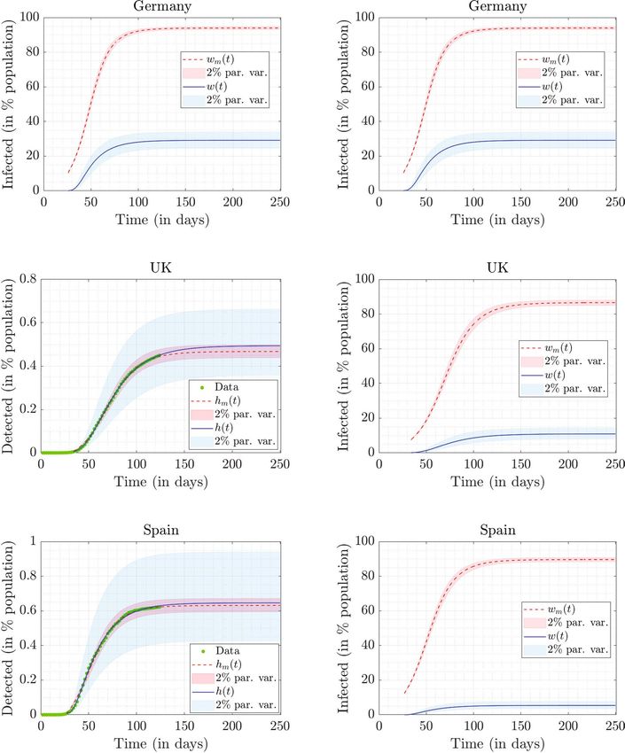
The best fits obtained using the two models for these three countries are presented in Fig. 3. For Germany (see
the top-left panel of Fig. 3), the continuum model under-predicts and for Spain (see the bottom-left panel of
Fig. 3), the continuum model over-predicts the actual data near the end. However, for the UK (see the mid-left
panel of Fig. 3), the fit is excellent. The variation of E0m obtained from the mean-β model in the p̄m − τm plane
(with βm and V0 fixed at values reported in Table 3) is plotted on the left panels of Fig. 4. The variation of E0
obtained from the continuum model in the p̄ − τ plane (with a, m and f0 fixed at values reported in Table 4) is
plotted on the right panels of Fig. 4. The affected-to-detected (A/D) ratio corresponding to the best fits for the
mean-β model and the continuum model are reported in Tables 3 and 4, respectively.
We see that the fitting results are qualitatively similar to those obtained for Italy. However, there are a few
observations that stand out in the results for the continuum model as highlighted below:
• We see in Table 4 that the optimum value of m for Germany, the UK, and Spain is around 2.5. This indicates
that the infectivity distribution φ(β) for each of these countries has a fat tail as can be in Fig. 2. We see from
the figure that most of the population has small infectivity (low value of β ). However, these curves decay to
zero very slowly, since the first moment of φ(β) is infinite, i.e.
∞
βφ(β) dβ = ∞.
β=0
Such a distribution is consistent with the presence of ‘super-spreaders’ (people who have, or events that lead
to, a high value of β ). Our results are in line with findings of Wong et al.28 that the distribution of infections
caused by an index case is fat-tailed. The role played by different kinds of super-spreading events, and empiri-
cal evidence for their role in the COVID-19 pandemic, are discussed in detail by Althouse et al.29 (see also
references therein). See the works by Adam et al.30 and Britton et al.31 for mathematical models discussing
the role of super-spreading in COVID-19. Super-spreading events have been widely reported for COVID-19
in the medical literature as well32,33.
• We see from Table 4 that the affected-to-detected ratio (A/D) is high for all the countries and varies between
8 for Spain and 130 for Germany.
• The ratio of symptomatic cases to detected cases can be approximated from the value of p. Symptomatic cases
outnumber the reported cases by about 5 times in Spain, 12 times in the UK, 25 times in Italy, and 60 times
in Germany.
• The serological study by Pollán et al.8 in Spain was carried out between April 27 and May 11, and about
61,000 people participated in it. It reports a seroprevalence of 5.0%(4.7 − 5.4) by the point-of-care test and
4.6%(4.3 − 5.0) by immunoassay. Our continuum model predicts that 4.04% and 4.65% of the Spanish popu-
lation was infected on April 27 and May 11, respectively. In the UK, 6.8%(5.2 − 8.6) of the population was
affected by COVID-19 as of May 2 434. Our continuum model predicts this number to be 8.63%. We could not
find a comparable nationwide study for Germany. Several studies are underway, but their results are not as
yet published35. However, the match with limited s tudies36,37 in Germany is poor, possibly because Germany’s
partial lockdown approach requires different modeling, e.g., a model with spatial structure.
Conclusions
In this work, we fit the data for the total number of infected people in four western European countries. We use
two limiting cases of the time-delayed network SEIQR model: the mean-β model and the continuum model. In
earlier works, it was shown that for fast pandemics, each of these two models reduces to one non-linear delay
differential equation.
After fixing the values of the biological parameters σ and γ , we need to identify four parameters in the mean-
β model and five parameters in the continuum model. In both the cases, we see that there are many parameter
sets that minimize the fitting error, yielding almost identical values of the objective function. All these sets have
almost identical values of all parameters other than p and τ . Other subsidiary quantities such as the total number
of infected people, the affected-to-detected ratio, and the basic reproduction number are also close to each other
in value. By plotting the fitting error in the p − τ plane (with other parameters fixed at their identified values), we
see that a narrow band yielding minimum error cuts across this plane, spanning the entire assumed range of τ and
a small range of p comprising low values. In this light, the τ values reported in Tables 3 and 4 may not be reliable.
We see from the results that the continuum model yields superior fits in comparison to the mean-β model.
Even the worst fit obtained from the continuum model, for Spain, has 2-norm fitting error of only 1.28%. Moreo-
ver, it gives reasonable and physically realizable values for all the epidemiological quantities. We conclude from
the results that the predicted number of infected people depends on the assumed distribution of the infectivity
rate. A single homogeneous infectivity rate overestimates the seroprevalence in the countries examined.
Both the models are relatively insensitive to small changes in the input parameters. The continuum model
is more sensitive than the mean-β model, which indicates indirectly that its parameter estimates are somewhat
more robust.
The most important prediction from the models is that the total number of affected people far outnum-
ber the people detected with COVID-19 in all the four countries. The continuum model predicts that the
affected-to-detected ratio, in increasing order, is 8, 22, 48, and 130 for Spain, the UK, Italy, and Germany,
Scientific Reports | (2021) 11:8106 | https://doi.org/10.1038/s41598-021-87630-z 8
Vol:.(1234567890)www.nature.com/scientificreports/
Figure 3. Top row: Fitted results for Germany, hm (250) = 0.2206%, h(250) = 0.2246%, wm (250) = 93.9666%
and w(250) = 29.1509%. Middle row: Fitted results for the UK, hm (250) = 0.4671%, h(250) = 0.4934%,
wm (250) = 86.6384% and w(250) = 10.9269%. Bottom row: Fitted results for Spain, hm (250) = 0.6311%,
h(250) = 0.6456%, wm (250) = 89.6423% and w(250) = 5.3903%. Data in percentage of population for detected
cases, obtained from Worldometer, is plotted using green circles. We have plotted the data of alternate days
for clarity. The fits obtained from the mean-β model are shown using dashed red curves, while those from the
continuum model are shown using solid blue curves. The parameters used in the mean-β model and continuum
model for obtaining the fit are shown in Tables 3 and 4, respectively. The red and blue shaded bands in all
the figures correspond to ±2% variations in the parameters in the mean-β model and the continuum model,
respectively.
Scientific Reports | (2021) 11:8106 | https://doi.org/10.1038/s41598-021-87630-z 9
Vol.:(0123456789)www.nature.com/scientificreports/
Figure 4. The left side shows the variation of E0m in the p̄m − τm plane (for low values of p̄m) obtained using
the mean-β model. The parameters βm and V0 are fixed at the values reported in Table 3. The right side shows
the variation of E0 in the p̄ − τ plane (for low values of p̄) obtained from the continuum model. The parameters
a, m, and f0 are fixed at the values reported in Table 4.
respectively. The first three of these numbers are consistent with the serological surveys conducted in the
corresponding countries. In particular, our estimated number of infected people in Spain in early May
was about 5% as per our model, in agreement with a nation-wide seroprevalence study 8. We emphasize
that the detailed work done in this seroprevalence study retains primary importance. Our work provides a
mathematical supporting view of consistency, and is not intended to replace such detailed seroprevalence
studies. Our numbers for affected people in Italy and the UK match reasonably well with seroprevalence
data from these c ountries27,34. In contrast however, our predicted numbers for Germany are too high. This
may be because the partial lockdown approach of Germany requires spatial structure within the model.
Scientific Reports | (2021) 11:8106 | https://doi.org/10.1038/s41598-021-87630-z 10
Vol:.(1234567890)www.nature.com/scientificreports/
Data availability
All the calculations were done in Matlab. The codes and the data can be found at: https://doi.o
rg/1 0.5 281/z enodo.
4419975.
Received: 7 October 2020; Accepted: 26 March 2021
References
1. Li, R. et al. Substantial undocumented infection facilitates the rapid dissemination of novel coronavirus (SARS-CoV-2). Science
368(6490), 489–493 (2020).
2. Flaxman, S. et al. Estimating the effects of non-pharmaceutical interventions on COVID-19 in Europe. Nature 584, 257–261 (2020).
3. Unwin, H. J. T. et al. State-level tracking of COVID-19 in the United States. Nat. Commun. 11, 6189 (2020).
4. Shekatkar, S. et al. INDSCI-SIM A State-level Epidemiological Model for India. Ongoing study at https://indscicov.in/indscisim
(2020).
5. Roser, M., Ritchie, H., Ortiz-Ospina, E. & Hasell, J. Coronavirus Pandemic (COVID-19). Our World in Datahttps://ourworldin
data.org/coronavirus (2020).
6. Bohk-Ewald, C., Dudel, C. & Myrskylä, M. A demographic scaling model for estimating the total number of COVID-19 infections.
Preprint at https://doi.org/10.1101/2020.04.23.20077719 (2020).
7. Scudellari, M. How the pandemic might play out in 2021 and beyond. Nature 584, 22–25 (2020).
8. Pollán, M. et al. Prevalence of SARS-CoV-2 in Spain (ENE-COVID): a nationwide, population-based seroepidemiological study.
Lancet 396(10250), 535–544 (2020).
9. Havers, F. P. et al. Seroprevalence of antibodies to SARS-CoV-2 in 10 sites in the United States, March 23-May 12, 2020. JAMA
Intern. Med. 180(12), 1576–1586 (2020).
10. https://www.gov.uk/government/publications/national-covid-19-surveillance-reports/sero-surveillance-of-covid-19 (2020)
11. https://indianexpress.com/article/cities/delhi/delhi-serological-survey-covid-19-icmr-6516208/ (2020)
12. Meunier, T. Full Lockdown Policies in Western Europe Countries Have No Evident Impacts on the COVID-19 Epidemic. Preprint
at https://doi.org/10.1101/2020.04.24.20078717 (2020).
13. Young, L. S., Ruschel, S., Yanchuk, S. & Pereira, T. Consequences of delays and imperfect implementation of isolation in epidemic
control. Sci. Rep. 9, 3505 (2019).
14. Vyasarayani, C. P. & Chatterjee, A. Complete dimensional collapse in the continuum limit of a delayed SEIQR network model with
separable distributed infectivity. Nonlinear Dyn. 101, 1653–1665 (2020).
15. Vyasarayani, C. P. & Chatterjee, A. New approximations, and policy implications, from a delayed dynamic model of a fast pandemic.
Physica D 414, 132701 (2020).
16. Barrat, A., Barthélemy, M. & Vespignani, A. Dynamical Processes on Complex Networks (Cambridge University Press, 2008).
17. Barabási, A. L. Network Science (Cambridge University Press, 2016).
18. https://www.worldometers.info/coronavirus/ (2020).
19. Barrat, A., Barthelemy, M., Pastor-Satorras, R. & Vespignani, A. The architecture of complex weighted networks. PNAS 101(11),
3747–3752 (2004).
20. Pastor-Satorras, R., Castellano, C. Van., Mieghem, P. & Vespignani, A. Epidemic processes in complex networks. Rev. Mod. Phys.
87(3), 925–979 (2015).
21. Saumell-Mendiola, A., Serrano, M. Á. & Bogunài, M. Epidemic spreading on interconnected networks. Phys. Rev. E 86(2), 026106
(2012).
22. Linka, K., Peirlinck, M., Sahli, C. F. & Kuhl, E. Outbreak dynamics of COVID-19 in Europe and the effect of travel restrictions.
Comput. Methods Biomech. Biomed. Eng. 23(11), 710–717 (2020).
23. Park, S. W. et al. Reconciling early-outbreak estimates of the basic reproductive number and its uncertainty: framework and
applications to the novel coronavirus (SARS-CoV-2) outbreak. J. R. Soc. Interface 17, 20200144 (2020).
24. Giordano, G. et al. Modelling the COVID-19 epidemic and implementation of population-wide interventions in Italy. Nat. Med.
26, 855–860 (2020).
25. Arnold, B. C. Pareto distribution in Wiley StatsRef: Statistics Reference. Online 1–10, https://doi.org/10.1002/9781118445112.
stat01100.pub2 (2015).
26. Rossa, F. D. et al. A network model of Italy shows that intermittent regional strategies can alleviate the COVID-19 epidemic. Nat.
Commun. 11, 5106 (2020).
27. Stefanelli, P. et al. Prevalence of SARS-CoV-2 IgG antibodies in an area of northeastern Italy with a high incidence of COVID-19
cases: a population-based study. Clin. Microbiol. Infect.https://doi.org/10.1016/j.cmi.2020.11.013 (2020).
28. Wong, F. & Collins, J. J. Evidence that coronavirus superspreading is fat-tailed. PNAS 117(47), 29416–29418 (2020).
29. Althouse, B. M. et al. Superspreading events in the transmission dynamics of SARS-CoV-2: opportunities for interventions and
control. PLoS Biol. 18(11), e3000897 (2020).
30. Adam, D. C. et al. Clustering and superspreading potential of SARS-CoV-2 infections in Hong Kong. Nat. Med. 26, 1714–1719
(2020).
31. Britton, T., Ball, F. & Trapman, P. A mathematical model reveals the influence of population heterogeneity on herd immunity to
SARS-CoV-2. Science 369(6505), 846–849 (2020).
32. https://www.washingtonpost.com/graphics/2020/world/coronavirus-south-korea-church/ (2020)
33. https://www.scientificamerican.com/article/how-superspreading-events-drive-most-covid-19-spread1/ (2020)
34. Colbourn, T. Unlocking UK COVID-19 policy. Lancet Public Health 5(7), E362–E363 (2020).
35. www.rki.de/covid-19-serostudiesgermany (2020).
36. Claudia, S. H. et al. Serology- and PCR-based cumulative incidence of SARS-CoV-2 infection in adults in a successfully contained
early hotspot (CoMoLo study), Germany, May to June 2020. Euro Surveill.https://doi.org/10.2807/1560-7917.ES.2020.25.47.20017
52 (2020).
37. Streeck, H. et al. Infection fatality rate of SARS-CoV2 in a super-spreading event in Germany. Nat. Commun. 11, 5829 (2020).
Author contributions
A.C. conceptualized the problem and supervised the overall research. S.T. and C.P.V generated all the figures
and wrote the preliminary manuscript. A.C. reviewed and edited the manuscript.
Competing interests
The authors declare no competing interests.
Scientific Reports | (2021) 11:8106 | https://doi.org/10.1038/s41598-021-87630-z 11
Vol.:(0123456789)www.nature.com/scientificreports/
Additional information
Supplementary Information The online version contains supplementary material available at https://doi.org/
10.1038/s41598-021-87630-z.
Correspondence and requests for materials should be addressed to C.P.V.
Reprints and permissions information is available at www.nature.com/reprints.
Publisher’s note Springer Nature remains neutral with regard to jurisdictional claims in published maps and
institutional affiliations.
Open Access This article is licensed under a Creative Commons Attribution 4.0 International
License, which permits use, sharing, adaptation, distribution and reproduction in any medium or
format, as long as you give appropriate credit to the original author(s) and the source, provide a link to the
Creative Commons licence, and indicate if changes were made. The images or other third party material in this
article are included in the article’s Creative Commons licence, unless indicated otherwise in a credit line to the
material. If material is not included in the article’s Creative Commons licence and your intended use is not
permitted by statutory regulation or exceeds the permitted use, you will need to obtain permission directly from
the copyright holder. To view a copy of this licence, visit http://creativecommons.org/licenses/by/4.0/.
© The Author(s) 2021
Scientific Reports | (2021) 11:8106 | https://doi.org/10.1038/s41598-021-87630-z 12
Vol:.(1234567890)You can also read