Modeling and Recognition of Landmark Image Collections Using Iconic Scene Graphs
←
→
Page content transcription
If your browser does not render page correctly, please read the page content below
Modeling and Recognition of Landmark Image
       Collections Using Iconic Scene Graphs

     Xiaowei Li, Changchang Wu, Christopher Zach, Svetlana Lazebnik, and
                             Jan-Michael Frahm

              Dept. of Computer Science, University of North Carolina
                           Chapel Hill, NC 27599-3175
               {xwli, ccwu, cmzach, lazebnik, jmf}@cs.unc.edu

       Abstract. This paper presents an approach for modeling landmark sites
       such as the Statue of Liberty based on large-scale contaminated image
       collections gathered from the Internet. Our system combines 2D appear-
       ance and 3D geometric constraints to efficiently extract scene summaries,
       build 3D models, and recognize instances of the landmark in new test im-
       ages. We start by clustering images using low-dimensional global “gist”
       descriptors. Next, we perform geometric verification to retain only the
       clusters whose images share a common 3D structure. Each valid cluster
       is then represented by a single iconic view, and geometric relationships
       between iconic views are captured by an iconic scene graph. In addition
       to serving as a compact scene summary, this graph is used to guide struc-
       ture from motion to efficiently produce 3D models of the different aspects
       of the landmark. The set of iconic images is also used for recognition,
       i.e., determining whether new test images contain the landmark. Results
       on three data sets consisting of tens of thousands of images demonstrate
       the potential of the proposed approach.

1    Introduction
The recent explosion in consumer digital photography and the phenomenal
growth of photo-sharing websites such as Flickr.com have created a high de-
mand for computer vision techniques for creating effective visual models from
large-scale Internet-based image collections. Given a large database of images
downloaded using a keyword search, the challenge is to identify all photos that
represent the concept of interest and to build a coherent visual model of the
concept despite heavy contamination by images with wrongly associated tags.
    Recent literature contains a number of approaches that address the problem
of visual learning from Internet image collections for general object categories
(see, e.g., [1–3]). These approaches are well-adapted to deal with label uncer-
tainty and make effective use of statistical appearance-based modeling, but lack
strong geometric constraints that are needed for modeling categories with a com-
mon rigid 3D structure, such as famous tourist sites and landmarks. For model-
ing and visualization of landmarks from Internet images, structure-from-motion
methods methods have been proposed [4, 5]. These methods employ powerful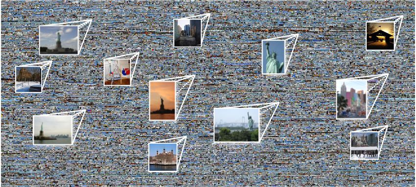
2      X. Li, C. Wu, C. Zach, S. Lazebnik and J.-M. Frahm

geometric constraints and produce compelling 3D reconstructions, but are cur-
rently not very scalable and not well suited to take advantage of more than a
small subset of a large and noisy community photo collection.
    This paper presents a hybrid approach that combines the strengths of 2D
recognition and 3D reconstruction for representing landmarks based on images
downloaded from Flickr.com using keyword searches. Our system proceeds in
an incremental fashion, initially applying 2D appearance-based constraints to
loosely group images, and progressively refining these groups with geometric con-
straints to select iconic images for a sparse visual summary of the scene. These
images and the pairwise geometric relationships between them define an iconic
scene graph that captures all the salient aspects of the landmark. The iconic scene
graph is then used for efficient reconstruction of a 3D skeleton model which can
also be extended to many more relevant images to a comprehensive “collective
representation” of the scene. The process of registering new test images to the
model also allows us to answer the recognition question, namely, whether the
landmark of interest is visible in a new test image. In addition, the iconic scene
graph can be used to organize the image collection into a hierarchical browsing
system. Because our method prunes many spurious images using fast 2D con-
straints and applies computationally demanding geometric constraints to just a
small subset of “promising” images, it is scalable to large photo collections.

2   Previous Work

This paper offers a comprehensive solution to the problems of dataset collection,
3D reconstruction, scene summarization, browsing and recognition for landmark
images. Below, we discuss related recent work in these areas.
    The problem of dataset collection refers to the following: starting with the
heavily contaminated output of an Internet image search query, extract a high-
precision subset of images that are actually relevant to the query. Existing ap-
proaches to this problem [1–3] consider general visual categories not necessarily
related by rigid 3D structure. They use statistical models to combine different
kinds of 2D image features (texture, color, keypoints), as well as text and tags.
However, 2D features alone do not provide strong enough constraints when ap-
plied to landmark images. Given the amount of clutter, viewpoint change, and
lighting variation typically present in consumer snapshots, as well as the unre-
liability of user-supplied tags, it is difficult to answer the question of whether a
landmark is actually present in a given picture without bringing in structure-
from-motion (SFM) constraints.
    The Photo Tourism system of Snavely et al. [5] uses SFM constraints very
effectively for modeling and visualization of landmarks. This system achieves
high-quality reconstruction results with the help of exhaustive pairwise image
matching and global bundle adjustment after inserting each new view. Unfortu-
nately, this process becomes very computationally expensive for large data sets,
and it is especially inefficient for heavily contaminated collections, most of whose
images cannot be registered to each other. Accordingly, the input images used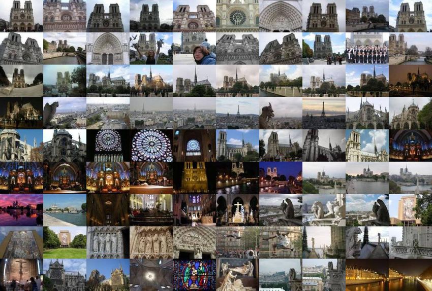
Iconic Scene Graphs       3

by Photo Tourism have either been acquired specifically for the task, or down-
loaded and pre-filtered by hand. When faced with a large and heterogeneous
dataset, the best this method can do is use brute force to reduce it to a small
subset that gives a good reconstruction. For example, for the Notre Dame results
reported in [5] 2,635 images of Notre Dame were used initially, and out of these,
597 images were successfully registered after about two weeks of processing.
    More recently, several researchers have developed SFM methods that exploit
the redundancy in community photo collections to make reconstruction more
efficient. In particular, many landmark image collections consist of a small num-
ber of “hot spots” from which photos are taken. Ni et al. [6] have proposed an
out-of-core bundle adjustment approach that takes advantage of this by locally
optimizing the “hot spots” and then connecting the local solutions into a global
one. In this paper, we follow a similar strategy of computing separate 3D re-
constructions on connected sub-components of the scene, thus avoiding the need
for frequent large-scale bundle adjustment. Snavely et al. [7] find skeletal sets of
images from the collection whose reconstruction provides a good approximation
to a reconstruction involving all the images. Similarly, our method is based on
finding a small subset of iconic images that capture all the important aspects
of the scene. However, unlike [6, 7], we rely on 2D appearance similarity as a
“proxy” or a rough approximation of the “true” multi-view relationship, and
our goals are much broader: in addition to reconstruction, we are also interested
in summarization, browsing, and recognition.
    The problem of scene summarization for landmark image collections has been
addressed by Simon et al. [8], who cluster images based on the output of exhaus-
tive pairwise feature matching. While this solution is effective, it is perhaps too
“strong” for the problem, as in many cases, a good subset of representative or
“iconic” images can be obtained for a scene using much simpler 2D techniques [9].
This is the philosophy followed in our work: instead of treating scene summa-
rization as a by-product of SFM, we treat it as a first step toward efficiently
computing the scene structure.
    Another problem relevant to our work is that of retrieval: given a query image,
find all images containing the same landmark in some target database [10, 11].
In this paper, we use retrieval techniques such as fast feature-based indexing
and geometric verification with RANSAC to establish geometric relationships
between different iconic images and to register a new test image to the iconics
for the purpose of recognition.

3   The Approach

In this section, we present the components of our implemented system. Figure 1
gives a high-level summary of these components, and Figure 2 illustrates them
with results on the Statue of Liberty dataset.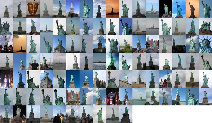
4          X. Li, C. Wu, C. Zach, S. Lazebnik and J.-M. Frahm

    1. Initial clustering (Section 3.1): Use “gist” descriptors to cluster the collection
       into groups roughly corresponding to similar viewpoints and scene conditions.
    2. Geometric verification and iconic image selection (Section 3.2): The goal
       of this stage is to filter out the clusters whose images do not share a common
       3D structure. This is done by pairwise epipolar geometry estimation among a few
       representative images selected from each cluster. The image that gathers the most
       inliers to the other representative images in its cluster is selected as the iconic
       image for that cluster.
    3. Construction of iconic scene graph (Section 3.3): Perform pairwise epipolar
       geometry estimation among the iconic images and create an iconic scene graph by
       connecting pairs of iconics that are related by a fundamental matrix or a homog-
       raphy. Edges are weighted by the number of inliers to the transformation.
    4. Tag-based filtering (Section 3.4): Use tag information to reject isolated nodes
       of the iconic scene graph that are semantically irrelevant to the landmark.
    5. 3D reconstruction (Section 3.5): First, partition the iconic scene graph into sev-
       eral tightly connected components and compute structure from motion separately
       on each component. Within each component, use a maximum spanning tree to de-
       termine the order of registering images to the model. At the end, merge component
       models along cut edges.
    6. Recognition (Section 4.2): Given a new test image, determine whether it contains
       an instance of the landmark. This can be done by efficiently registering the image
       to the iconics using appearance-based scores and geometric verification.

                    Fig. 1. Summary of the major steps of our system.

3.1      Initial Clustering
Our goal is to compute a representation of a landmark site by identifying a set
of canonical or iconic views corresponding to dominant scene aspects. Recently,
Simon et al. [8] have defined iconic views as representatives of dense clusters of
similar viewpoints. To find these clusters, Simon et al. take as input a feature-
view matrix (a matrix that says which 3D features are present in which views)
and define similarity of any two views in terms of the number of 3D features they
have in common. By constrast, we adopt a perceptual or image-based perspective
on iconic view selection: if there are many images in the dataset that share a
very similar viewpoint in 3D, then at least some of them will have a very similar
image appearance in 2D, and can be matched efficiently using a low-dimensional
global description of their pixel patterns.
    The global descriptor we use is gist [12], which was found to be effective for
grouping images by perceptual similarity [13]. We cluster the gist descriptors of
all our input images using k-means with k = 1200. Since at the next stage, we
will select at most a single iconic image to represent each cluster, we initially
want to produce an over-clustering to give us a large and somewhat redundant
set of candidate iconics. In particular, we can expect images with very similar
viewpoints to end up in different gist clusters because of clutter (i.e., people
in front of the camera), differences in lighting, or camera zoom. This does not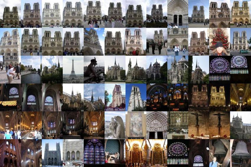
Iconic Scene Graphs        5

                     Statue of Liberty: 45284 images

                               196 iconic images

                                           Statue of Liberty
                                              (New York)

  Statue of Liberty                                             Statue of Liberty
     (Las Vegas)                                                     (Tokyo)

Fig. 2. A snapshot of the operation of our system for the Statue of Liberty. The ini-
tial dataset of 45284 images (of which about 40% are unrelated to the landmark) gets
reduced to a set of 196 iconics by 2D appearance-based clustering followed by geomet-
ric verification of top cluster representatives. The iconics are nodes in a scene graph
consisting of multiple connected components, each of which gives rise to a 3D recon-
struction. The largest reconstructed component corresponds to the Statue of Liberty
in New York, while two of the smaller ones correspond to copies of the statue in Tokyo
and Las Vegas. These components are found completely automatically. A video of the
models can also be found at http://www.cs.unc.edu/iconic-scene-graphs.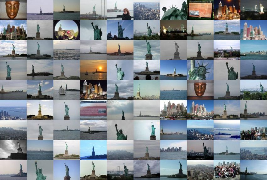
6       X. Li, C. Wu, C. Zach, S. Lazebnik and J.-M. Frahm

cause a problem for our approach, because the graph construction step of Section
3.3 will be able to restore links between different clusters that have sufficient
viewpoint similarity.
    In our experiments, we have found that the largest gist clusters tend to be
the cleanest ones. Therefore, for the initial stage, we use cluster size to produce a
first, coarse ranking of images. As shown in the quantitative evaluation in Figure
6(a) (Stage 1), the first few gist clusters have a surprisingly high precision, though
it deteriorates rapidly for subsequent clusters.

3.2   Geometric Verification and Iconic Image Selection

The next step is to perform verification of each gist cluster to confirm that its
images share a common 3D structure. To do this efficiently, we select a small
number of the most representative images from each cluster and attempt to
estimate the two-view geometry of every pair. The representatives are given
by n images (in our current implementation, n = 8) whose gist descriptors are
closest to the cluster mean. Note that gist clusters that have fewer than n images
are rejected before this step.
    For fitting a geometric transformation to these matches, we extract SIFT
features [14] and use QDEGSAC [15], which is a robust procedure that returns
an estimate for a fundamental matrix or a homography, depending on the scene
structure. The image that gathers the largest total number of inliers to the other
n − 1 representatives from its cluster is declared the iconic image of that cluster.
If any of the remaining representatives are not consistent with the iconic, we
remove them and attempt to replace them with other images from the same
cluster (within clusters, images are ranked in order of increasing distance from
the center). If at the end of this process we are not able to find n − 1 other
consistent images, the cluster is rejected.
    The inlier score of each iconic can be used as a new measure of the quality
of each cluster. Precision/recall curves in Figure 6(a) (Stage 2) demonstrate
that this ranking does a better job than gist alone in separating the relevant
images from the irrelevant ones. However, there is an undesirable effect of a
few geometrically consistent, but semantically irrelevant clusters getting very
high scores at this stage, which hurts precision early on. Such clusters typically
result from near-duplicate images coming from the same user’s photo album. As
described in the next section, we will be able to reject many such clusters using
inter-cluster matching and filtering based on tags.
    Ranking of clusters based on the top representatives does not penalize clus-
ters that have a few geometrically consistent images, but are very low-precision
otherwise. Once the iconic images for every cluster are selected, we can perform
geometric verification of every remaining image by matching it to the iconic of
its cluster and ranking it individually by the number of inliers it has with respect
to its iconic. As shown in Figure 6(a) (Stage 3), this individual ranking improves
precision considerably.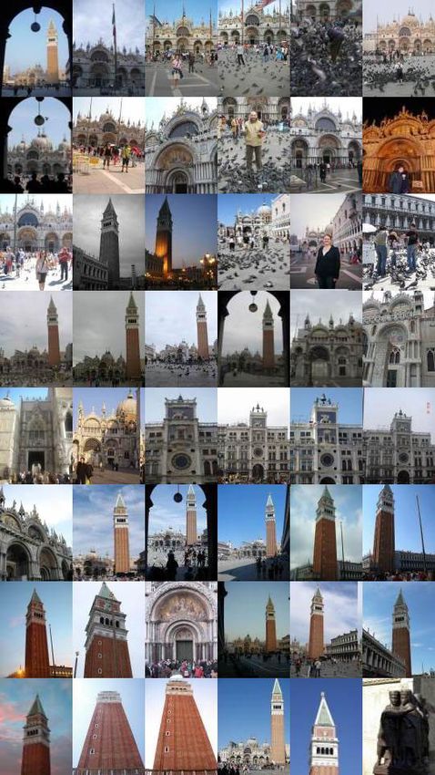
Iconic Scene Graphs       7

3.3   Construction of Iconic Scene Graph

Next, we need to establish links between the iconic images selected in the pre-
vious step. Since we have hundreds of iconic images even following rejection of
geometrically inconsistent clusters, exhaustive pairwise matching of all iconics
is still rather inefficient. To match different iconic images, we need to account
for larger viewpoint and appearance changes than in the initial clustering, so
keypoint-based methods are more appropriate for this stage. We use the vo-
cabulary tree method of Nister and Stewenius [16] as a fast indexing scheme
to obtain promising candidates for pairwise geometric verification. We train a
vocabulary tree with five levels and a branching factor of 10 using a set of thou-
sands of frames taken from a video sequence of urban data, and populate it with
SIFT features extracted from our iconics. We then use each iconic as a query
image and perform geometric verification with top 20 other iconics returned by
the vocabulary tree. Pairs of iconics that match with more than 18 inliers are
then connected by an edge whose weight is given by the inlier score. This re-
sults in an undirected, weighted iconic scene graph whose nodes corresond to
iconic views and edges correspond to two-view transformations (homographies
or fundamental matrices) relating the iconics.
    Next, we would like to identify a small number of strongly connected compo-
nents in the iconic scene graph. This serves two purposes. The first is to group
together iconics that are close in terms of viewpoint but did not initially fall
into the same gist cluster. The second is to obtain smaller subsets of images on
which structure from motion can be performed more efficiently. To partition the
graph, we use normalized cuts [17], which requires us to specify as input the
desired number of components. This parameter choice is not critical, since any
oversegmentation of the graph will be addressed by the component merging step
discussed in the next section. We have found that specifying a target number of
20 to 30 components produces acceptable results for all our datasets.
    Every (disjoint) component typically represents a distinctive aspect of the
landmark, and we can select a single representative iconic for each component
(i.e., the iconic with the highest sum of edge weights) to form a compact scene
summary. Moreover, the components of the iconic scene graph and the iconic
clusters induce a hierarchical structure on the dataset that can be used for
browsing, as shown in Figure 3.

3.4   Tag-Based Filtering

The iconic scene graph tends to have many isolated nodes, corresponding to
iconic views for which we could not find a geometric relationship with any other
view. These nodes are excluded from the graph partitioning process described
above. They may either be aspects of the scene that are significantly different
from others, e.g., the interior of the Notre Dame cathedral in Paris, or geomet-
rically consistent, but semantically irrelevant clusters, e.g., pictures of a Notre
Dame cathedral in a different city. Since constraints on appearance and geome-
try are not sufficient to establish the relationship of such clusters to the scene, to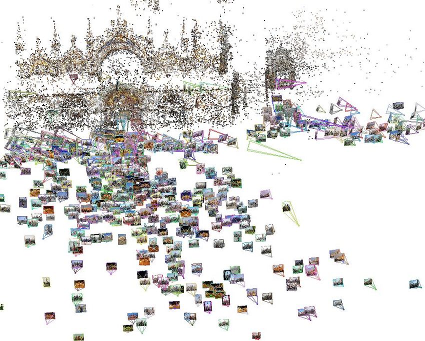
8       X. Li, C. Wu, C. Zach, S. Lazebnik and J.-M. Frahm

       Level 1                  Level 2

                                                                Level 3

Fig. 3. Hierarchical organization of the dataset for browsing. Level 1: components of
the iconic scene graph. Level 2: Each component can be expanded to show all the
iconic images associated with it. Level 3: each iconic can be expanded to show the
images associated with its gist cluster. Our three datasets may be browsed online at
http://www.cs.unc.edu/iconic-scene-graphs.

refine our dataset further we need to use additional information, in particular,
the tags associated with the images on Flickr.
    Even though Flickr tags in general tend to be quite unreliable, we have
observed that among the isolated clusters that have already been pre-filtered
by appearance and geometry constraints, there are quite a few whose tags are
clearly unrelated to the landmark. This suggests that, provided we have a good
idea of the distribution of relevant tags, a very simple score should be sufficient to
identify the “bad” clusters. Fortunately, during the previous modeling stages, we
have already verified hundreds of images without resorting to tags, so we can now
use these images to acquire the desired distribution. In the implementation, we
take iconic images that have at least two edges in the scene graph (empirically,
these are almost certain to contain the landmark), and use them to create a
“master list” of relevant tags. To have a more complete list, we also incorporate
tags from the top cluster images registered to these iconics. The tags in the list
are ranked in decreasing order of frequency, and isolated iconic images are scored
based on the median rank of their tags (tags that don’t occur in the master list at
all are assigned an arbitrary high number). Clusters with “obviously” unrelated
tags get a high median rank and can be removed to increase precision, as shown
by the “Stage 4” curves in Figure 6(a).

3.5   3D Reconstruction
As a first step, the 3D structure for every component produced by normalized
cuts is computed separately. Starting with a good initial image pair, we incre-
mentally add more views to the reconstruction by perspective pose estimation.
There are two criteria for selecting a good initial pair. First, in order to operate
in metric instead of projective space, the views in question require reasonable
estimates for the focal lengths, which can be obtained from EXIF data. When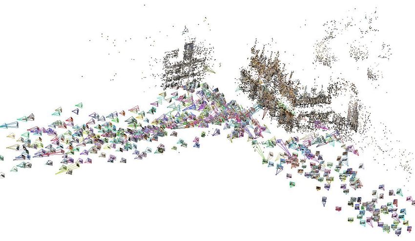
Iconic Scene Graphs         9

                          Modeling       Testing   All 3D models  Largest 3D model
  Dataset           Unlabeled Pos. Neg. Pos. Neg. #Models #Views #Views      #Pts
  Notre Dame             9760 545 535 541 503       8         580     337    30802
  Statue of Liberty     42983 1369 932 646 446      6        1068     871    18675
  San Marco             38332 2094 3131 379 715     4        1213     749    39307
Table 1. Summary statistics of our datasets and 3D models. The first five columns list
dataset sizes and numbers of labeled images. The next two columns give details of
our computed 3D models: the number of distinct models after merging and the total
number of registered views (these include both iconic and non-iconic images). The last
two columns refer to just the single largest 3D model. They list the number of registered
views and the number of 3D points visible in at least three views.

EXIF data is not available, we transfer the focal length estimate from similar
views in the same cluster. Second, the number of inlier correspondences should
be as large as possible, taking into account the 3D point triangulation certainty
(i.e. the shape of the covariance matrices) [18]. Once an initial pair of images
is found, their relative pose is determined by the five-point method [19]. The
remaining views of the current component are added using perspective pose es-
timation from 2D-3D correspondences. The order of insertion is determined from
the edges of the underlying maximum spanning tree computed for the weighted
graph component. Hence, views having more correspondences with the current
reconstruction are added first. The resulting 3D structure and the camera pa-
rameters are optimized by non-linear sparse bundle adjustment [20].
    The above reconstruction process applied to individual graph components
produces small individual models representing single aspects of the landmark.
A robust estimation of the 3D similarity transform is used to align and merge
suitable components and their respective reconstructions. This merging process
restores the connectivity of the original scene graph, and results in a single
“skeleton” 3D model for each original connected component. The last step is to
augment these models by incorporating additional non-iconic images from clus-
ters. Each image we consider for adding has already been successfully registered
with the iconic of its cluster, as described in Section 3.2. Since the features from
the iconic have already been incorporated into the skeleton 3D model, the regis-
tration between the image and the iconic gives us a number of 2D/3D matches
for that image. To obtain additional 2D/3D matches, we attempt to register this
new image to two additional iconics that are connected to its original iconic by
the highest-weight edges. All these matches are then used to estimate the pose
of the new image. At the end, bundle adjustment is applied to refine the model.

4     Experimental Results

4.1   Data Collection and Model Construction

We have tested our system on three datasets: the Notre Dame cathedral in
Paris, the Statue of Liberty in New York, and Piazza San Marco in Venice.
The datasets were automatically downloaded from Flickr.com using keyword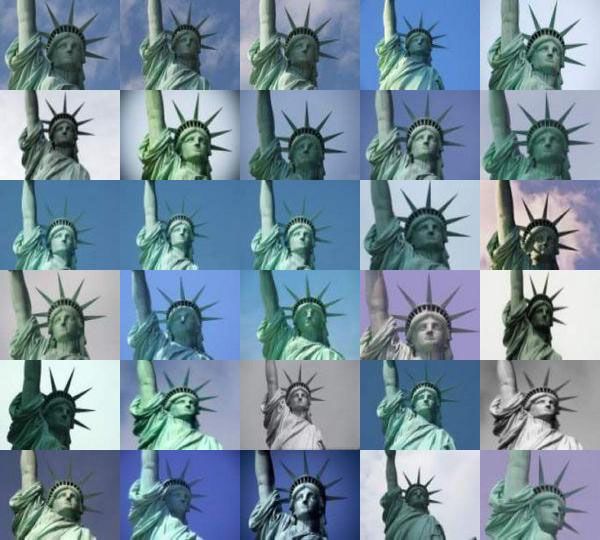
10      X. Li, C. Wu, C. Zach, S. Lazebnik and J.-M. Frahm

                          Notre Dame: 162 iconic images

        Front model (2 views)                       Rear model (2 views)

Fig. 4. Notre Dame results. Top: iconic images. Note that there are a few spurious
iconics corresponding to Notre Dame cathedrals in Indiana and Montreal (these were
not removed by the tag filtering step), as well as the Eiffel Tower seen from the top
of Notre Dame. Bottom: two of the reconstructed scene components, corresponding to
the front and back of the cathedral.

searches. We randomly split each dataset into a “modeling” part, and a much
smaller independent “testing” part. Because the modeling datasets contain tens
of thousands of images, we have chosen to label only a small randomly selected
fraction of them. These ground-truth labels are needed only to measure recall
and precision for the different stages of refinement, since our modeling approach
is completely unsupervised. The smaller test sets are completely labeled. Our
labeling is very basic, merely recording whether the landmark is present in the
image or not, without evaluating the “quality” or “typicality” of a given view.
For example, interior views of Notre Dame are labeled as positive, even though
they are relatively few in number and cannot be registered to the exterior views.
Table 1 gives a breakdown of the numbers of labeled and unlabeled images in
our datasets. The proportions of negative images (40% to 60%) give a good idea
of the initial amount of contamination.
    Figure 6(a) shows recall/precision curves for the modeling process on the
three datasets. We can see that the four refinement stages (gist clustering, geo-
metric verification of clusters, verification of individual images w.r.t. their cluster
centers, and tag-based rejection) progressively increase the precision of the im-
ages selected as part of the model, even though recall decreases following the
rejection decisions made after every stage.
Iconic Scene Graphs 11
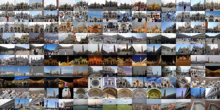
San Marco: 198 iconic images
Model 1 (2 views) Model 2
Fig. 5. San Marco results. Top: iconic images. Bottom: two of the reconstructed scene
components, corresponding to the front and the back of the square.
Figures 2, 4 and 5 show the reconstructed 3D models for our three datasets
(see http://www.cs.unc.edu/iconic-scene-graphs for videos of the models).
As described in Section 3.5, reconstruction is first performed on separate compo-
nents of the iconic scene graph, followed by merging of models with sufficiently
overlapping scene components. Successful merging requires images that link the
component models. For San Marco, the merging of the models corresponding to
the front and back of the square was not successful because the iconic images
did not provide a sufficient coverage of the middle region. For a similar reason,
it was not possible to merge the front and the back of Notre Dame. To an ex-
tent, this merging problem is endemic to community photo collections, as people
tend to take snapshots of famous landmarks from a small number of particu-
larly characteristic or accessible “hot spots,” while the areas in between remain
sparsely covered. Our clustering approach may in some cases exacerbate this
problem by discarding the less common images that fail to produce sufficiently
large clusters. Despite the difficulty of merging, our models successfully incor-
porate a significant number of images, as shown in Table 1. While our models
currently do not exceed in size those produced by the Photo Tourism system [5],
we are able to process an order of magnitude more images with just a fraction12 X. Li, C. Wu, C. Zach, S. Lazebnik and J.-M. Frahm
of the computational power, i.e., hours on a single commodity PC, instead of
weeks on a high-performance cluster.
4.2 Testing and Recognition
Given a new image that was not in our initial collection, we want to find out
whether it contains the landmark of interest. A straightforward of doing this
is by retrieving the iconic image that gets the highest matching score with the
test image (according to a given retrieval scheme) and making the yes/no deci-
sion by setting a threshold on the retrieval score. We can evaluate performance
quantitatively by plotting a recall/precision curve of the test images ordered
from highest to lowest score. Figure 6 (b) and (c) shows the results for several
retrieval strategies. The simplest strategy is to compare the test image to the
iconics using either gist descriptors (in which case the score would be inversely
proportional to the distance) or a bag-of-features representation using the vo-
cabulary tree (which returns a tf/idf score [16]). For improved performance, we
can take top k “candidate” iconics retrieved with either gist or vocabulary tree,
and perform geometric verification with each candidate as described in Section
3.2. In this case, the score for each candidate is the number of inliers to a two-
view transformation (homography or fundamental matrix) between it and the
test image, and only the top candidate is retained.
Interestingly, for the Statue of Liberty, the performance of the vocabulary tree
without geometric verification is almost disastrous. This is due to the relative
lack of texture in many Statue of Liberty images, which gives too few local
features for bag-of-words matching to work reliably. But in most other cases,
gist and vocabulary tree have comparable performance. Not surprisingly, for
both kinds of image description, geometric verification significantly improves
accuracy, as does retrieving more candidates for verification. For comparison,
we also include a recall/precision curve for scoring test images based on their
tag relevance (see Section 3.4). By itself, this scoring scheme is quite unreliable.
5 Discussion
We have presented a hybrid approach combining 2D appearance and 3D ge-
ometry to efficiently model and recognize complex real-world scenes captured
by thousands of amateur photos. To our knowledge, our system is the first in-
tegrated solution to the problems of dataset collection, scene summarization,
browsing, 3D reconstruction, and recognition for landmark images. At the heart
of our approach is the iconic scene graph, which captures the major aspects of
the landmark and the geometric connections between them. The structure of this
graph is used, among other things, to create a three-level browsing hierarchy and
to enable scalable computation of structure from motion.
In the future, one of our main goals is to improve the recall of our modeling
process. This can be done by making use of fast and accurate retrieval techniques
such as [10, 11] to re-incorporate images that were discarded during the iconicIconic Scene Graphs 13
(a) (b) (c)
Notre Dame Modeling Notre Dame Testing − GIST Notre Dame Testing − VocTree
1.1 1.1 1.1
1 1 1
0.9 0.9 0.9
0.8 0.8 0.8
0.7 0.7 0.7
Precision
Precision
Precision
0.6 0.6 0.6
0.5 0.5 0.5
0.4 0.4 0.4
0.3 0.3 Tag 0.3 Tag
Stage 1 GIST 1NN VocTree 1NN
0.2 Stage 2 0.2 GIST 1NN+Match
0.2 VocTree 1NN+Match
0.1 Stage 3 0.1 GIST 5NN+Match 0.1 VocTree 5NN+Match
Stage 4 GIST 10NN+Match VocTree 10NN+Match
0 0 0
0 0.1 0.2 0.3 0.4 0.5 0.6 0.7 0.8 0.9 1 0 0.2 0.4 0.6 0.8 1 0 0.2 0.4 0.6 0.8 1
Recall Recall Recall
Statue of Liberty Modeling Statue of Liberty Testing − GIST Statue of Liberty Testing − VocTree
1.1 1.1 1.1
1 1 1
0.9 0.9 0.9
0.8 0.8 0.8
0.7 0.7 0.7
Precision
Precision
Precision
0.6 0.6 0.6
0.5 0.5 0.5
0.4 0.4 0.4
0.3 0.3 Tag 0.3 Tag
Stage 1 GIST 1NN VocTree 1NN
0.2 Stage 2 0.2 GIST 1NN+Match
0.2 VocTree 1NN+Match
0.1 Stage 3 0.1 GIST 5NN+Match 0.1 VocTree 5NN+Match
Stage 4 GIST 10NN+Match VocTree 10NN+Match
0 0 0
0 0.1 0.2 0.3 0.4 0.5 0.6 0.7 0.8 0.9 1 0 0.2 0.4 0.6 0.8 1 0 0.2 0.4 0.6 0.8 1
Recall Recall Recall
San Marco Modeling San Marco Testing − GIST San Marco Testing − VocTree
1.1 1.1 1.1
1 1 1
0.9 0.9 0.9
0.8 0.8 0.8
0.7 0.7 0.7
Precision
Precision
Precision
0.6 0.6 0.6
0.5 0.5 0.5
0.4 0.4 0.4
0.3 0.3 Tag 0.3 Tag
Stage 1 GIST 1NN VocTree 1NN
0.2 Stage 2 0.2 0.2
GIST 1NN+Match VocTree 1NN+Match
0.1 Stage 3 0.1 GIST 5NN+Match 0.1 VocTree 5NN+Match
Stage 4 GIST 10NN+Match VocTree 10NN+Match
0 0 0
0 0.1 0.2 0.3 0.4 0.5 0.6 0.7 0.8 0.9 1 0 0.2 0.4 0.6 0.8 1 0 0.2 0.4 0.6 0.8 1
Recall Recall Recall
Fig. 6. Recall/precision curves for (a) modeling; (b) testing with the gist descriptors;
and (c) testing with the vocabulary tree. For modeling, the four stages are as follows.
Stage 1: Clustering using gist and ranking each image by the size of its gist cluster
(Section 3.1). Stage 2: Geometric verification of iconics and ranking each image by
the inlier number of its iconic (Section 3.2). The recall is lower because inconsistent
clusters are rejected. Stage 3: Registering each image to its iconic and ranking the
image by the number of inliers of the two-view transformation to the iconic. Unlike in
the first two stages, images are no longer arranged by cluster, but ranked individually
by this score. The recall is lower because images with not enough inliers to estimate
a two-view transformation are rejected. Stage 4: Tag information is used to retain
only the top 30 isolated clusters (Section 3.4). The score is the same as in stage 3,
except that images belonging to the rejected clusters are removed. Note the increase in
precision in the first few retrieved images. For testing, the different retrieval strategies
are as follows. GIST 1NN (resp. VocTree 1NN): retrieval of the single nearest
iconic using the gist descriptor (resp. vocabulary tree); GIST kNN+Match (resp.
VocTree kNN+Match): retrieval of k nearest exemplars using gist (resp. vocabulary
tree) followed by geometric verification; Tag: tag-based ranking (see Section 3.4).14 X. Li, C. Wu, C. Zach, S. Lazebnik and J.-M. Frahm
image selection stage. A similar strategy could also be helpful for discovering
“missing links” for merging 3D models of different components. In addition, we
plan to create 3D models that incorporate a much larger number of images. This
will require a memory-efficient streaming approach for registering new images,
as well as out-of-core bundle adjustment using iconic scene graph components.
References
1. Fergus, R., Perona, P., Zisserman, A.: A visual category filter for Google images.
In: ECCV. (2004)
2. Berg, T., Forsyth, D.: Animals on the web. In: CVPR. (2006)
3. Schroff, F., Criminisi, A., Zisserman, A.: Harvesting image databases from the
web. In: ICCV. (2007)
4. Goesele, M., Snavely, N., Curless, B., Hoppe, H., Seitz, S.M.: Multi-view stereo
for community photo collections. In: ICCV. (2007)
5. Snavely, N., Seitz, S.M., Szeliski, R.: Photo tourism: Exploring photo collections
in 3d. In: SIGGRAPH. (2006) 835–846
6. Ni, K., Steedly, D., Dellaert, F.: Out-of-core bundle adjustment for large-scale 3d
reconstruction. In: ICCV. (2007)
7. Snavely, N., Seitz, S.M., Szeliski, R.: Skeletal sets for efficient structure from
motion. In: CVPR. (2008)
8. Simon, I., Snavely, N., Seitz, S.M.: Scene summarization for online image collec-
tions. In: ICCV. (2007)
9. Berg, T.L., Forsyth, D.: Automatic ranking of iconic images. Technical report,
University of California, Berkeley (2007)
10. Chum, O., Philbin, J., Sivic, J., Isard, M., Zisserman, A.: Total recall: Automatic
query expansion with a generative feature model for object retrieval. In: ICCV.
(2007)
11. Philbin, J., Chum, O., Isard, M., Sivic, J., Zisserman, A.: Lost in quantization:
Improving particular object retrieval in large scale image databases. In: CVPR.
(2008)
12. Oliva, A., Torralba, A.: Modeling the shape of the scene: a holistic representation
of the spatial envelope. IJCV 42 (2001) 145–175
13. Hays, J., Efros, A.A.: Scene completion using millions of photographs. In: SIG-
GRAPH. (2007)
14. Lowe, D.: Distinctive image features from scale-invariant keypoints. IJCV 60
(2004) 91–110
15. Frahm, J.M., Pollefeys, M.: RANSAC for (quasi-)degenerate data (QDEGSAC).
In: CVPR. Volume 1. (2006) 453–460
16. Nister, D., Stewenius, H.: Scalable recognition with a vocabulary tree. In: CVPR.
(2006)
17. Shi, J., Malik, J.: Normalized cuts and image segmentation. PAMI 22 (2000)
888–905
18. Beder, C., Steffen, R.: Determining an initial image pair for fixing the scale of a
3d reconstruction from an image sequence. In: Proc. DAGM. (2006) 657–666
19. Nistér, D.: An efficient solution to the five-point relative pose problem. PAMI 26
(2004) 756–770
20. Lourakis, M., Argyros, A.: The design and implementation of a generic sparse
bundle adjustment software package based on the Levenberg-Marquardt algorithm.
Technical Report 340, Institute of Computer Science - FORTH (2004)You can also read