Submodular Dictionary Learning for Sparse Coding

Page created by Rene Holland
 
CONTINUE READING
Submodular Dictionary Learning for Sparse Coding
                            Zhuolin Jiang† , Guangxiao Zhang†§ , Larry S. Davis†
      †
        Institute for Advanced Computer Studies, University of Maryland, College Park, MD, 20742
               §
                 Global Land Cover Facility, University of Maryland, College Park, MD, 20742
                                      {zhuolin, gxzhang, lsd}@umiacs.umd.edu

                         Abstract                                dictionaries relevant to classification.
   A greedy-based approach to learn a compact and dis-               Generally, most dictionary learning algorithms [12, 35,
criminative dictionary for sparse representation is pre-         32, 21, 25, 27] iteratively alternate a sparse coding step (for
sented. We propose an objective function consisting of two       computing the sparse codes over the dictionary obtained at
components: entropy rate of a random walk on a graph             the previous iteration), with a dictionary update step given
and a discriminative term. Dictionary learning is achieved       the sparse codes from the previous sparse coding step. They
by finding a graph topology which maximizes the objec-           access the entire training set at each iteration in order to op-
tive function. By exploiting the monotonicity and submod-        timize the objective function. These algorithms converge
ularity properties of the objective function and the matroid     slowly when the reconstruction error is required to be small.
constraint, we present a highly efficient greedy-based op-       Moreover, they may get trapped in local minimum. Al-
timization algorithm. It is more than an order of magni-         though some algorithms [16, 22, 29] for efficient dictionary
tude faster than several recently proposed dictionary learn-     learning have been proposed recently, effectively solving
ing approaches. Moreover, the greedy algorithm gives a           the optimization problem for dictionary learning is still a
near-optimal solution with a (1/2)-approximation bound.          significant computational challenge.
Our approach yields dictionaries having the property that            Submodularity can be considered as a discrete analog
feature points from the same class have very similar sparse      of convexity. The diminishing return property of submod-
codes. Experimental results demonstrate that our approach        ularity has been employed in applications such as sensor
outperforms several recently proposed dictionary learning        placement [10], superpixel segmentation [19] and cluster-
techniques for face, action and object category recognition.     ing [36, 23]. In this paper, we present a supervised al-
                                                                 gorithm for efficiently learning a compact and discrimina-
1. Introduction                                                  tive dictionary for sparse representation. We define a novel
   Sparse coding represents an input signal y as a linear        monotonic and submodular objective function, which con-
combination of a few items from a dictionary, D. Learn-          sists of two terms: the entropy rate of a random walk on
ing the dictionary is critical for good performance. The         a graph and a discriminative term. The entropy rate term
SRC algorithm [30], for example, employs the entire set of       favors compact and homogeneous clusters, so each cluster
training samples as the dictionary and achieves impressive       center can well represent the cluster elements. The discrim-
performance on face recognition. For many applications,          inative term encourages the clusters to be class pure and
however, rather than using the entire set of training data       leads to a smaller number of clusters. Hence, each clus-
as dictionary, it is computationally advantageous to learn       ter center preserves category information and makes the
a compact dictionary from training data.                         computed sparse codes discriminative when using a dictio-
   Many algorithms [30, 1, 35, 12, 5] have been developed        nary consisting of all the cluster centers. As shown in Fig-
for learning such dictionaries. The dictionary in [30] is        ures 1(b) and 2(b), the dictionaries learned by our approach
manually selected from the training samples. [1] proposes        encourage the sparse codes for signals from the same class
the K-SVD algorithm using orthogonal matching pursuit for        to be similar. The main contributions of this paper are:
sparse coding and learns an over-complete dictionary in a           • We model the problem of discriminative dictionary
reconstructive manner. The method of optimal directions                learning as a graph topology selection problem, which
(MOD) [5] shares the same sparse coding step but has a dif-            is solved by maximizing a monotonically increasing
ferent dictionary update process. These learning approaches            and submodular objective function.
have led to excellent results in image denoising and inpaint-       • We present a highly efficient greedy optimization ap-
ing [22, 1]. However, the dictionaries obtained by using               proach by using the submodularity and monotonic in-
the reconstructive formulation, while optimized for recon-             creasing properties of the objective function under a
struction, may not necessarily be best for classification. The         matroid constraint, that scales to large datasets.
reconstructive formulation can be augmented with discrim-           • We prove that the objective function is monotonically
inative terms [12, 35, 32, 21, 25], that encourage learning            increasing and submodular, and the cycle-free con-
Submodular Dictionary Learning for Sparse Coding
straint and the connected component constraint in the           Z = [z1 ...zN ] ∈ RK×N for Y are obtained by solving:
    graph partitioning induce a matroid. The proofs are                  Z = arg min kY − DZk22 s.t. ∀i, kzi k0 ≤ s (1)
    given in the supplementary material.                                             Z
                                                                    where kY − DZk22 denotes the reconstruction error and
  • Our approach achieves state of the art performance
                                                                    kzi k0 ≤ s is the sparsity constraint (that each signal has s
    on various public face, action and object recognition
                                                                    or fewer items in its decomposition). Orthogonal matching
    benchmarks.
                                                                    pursuit algorithm can be used to solve (1).
1.1. Related Work                                                      The performance of sparse representation depends criti-
   Discriminative dictionary learning algorithms have been          cally on D. SRC [30] constructs D by using all the training
the focus of recent research. Some algorithms learn mul-            samples; this can result in a very large dictionary, which
tiple dictionaries or category-dependent dictionaries [20,          makes subsequent sparse coding expensive. Thus, methods
33]. [20] constructs one dictionary per class and classifi-         for learning a small-size dictionary for sparse coding have
cation is based on the corresponding reconstruction errors.         been proposed. For example, the K-SVD algorithm [1] is
   Some algorithms learn a dictionary by merging or select-         well-known for efficiently learning an over-complete dic-
ing dictionary items from a large set of dictionary item can-       tionary from a set of training signals; it solves:
didates [18, 14, 26, 13]. [18, 14] learn a dictionary through         < D, Z >= arg min kY −DZk22 s.t. ∀i, kzi k0 ≤ s (2)
                                                                                         D,Z
merging two items by maximizing the mutual information
of class distributions. [13] constructs a dictionary for signal     where D = [d1 ...dK ] ∈ Rn×K is the learned dictionary,
reconstruction from a set of dictionary item candidates. The        and Z are the sparse representations of Y .
objective function in [13] satisfies approximate submodu-               However, K-SVD only focuses on minimizing the recon-
larity under a certain incoherence assumption on the candi-         struction error and does not consider the dictionary’s util-
date elements. For these approaches, a large dictionary is          ity for discrimination. The discrimination power should be
required at the beginning to guarantee discriminative power         considered when constructing dictionaries for classification
of the constructed compact dictionary.                              tasks. Some discriminative approaches [25, 35, 12, 21, 32],
   Some algorithms add discriminative terms into the objec-         which add extra discriminative terms into the cost function
tive function of dictionary learning [27, 35, 12, 32, 21, 25].      for classification task, have been investigated.
The discriminative terms include Fisher discrimination cri-             However, these approaches appear to require large dic-
terion [27], linear predictive classification error [35, 25], op-   tionaries to achieve good performance, leading to high com-
timal sparse coding error [12], softmax discriminative cost         putation cost especially when additional terms are added
function [21] and hinge loss function [32].                         into the objective function. The computation requirements
   In addition, submodularity has been exploited for clus-          are further aggravated when good classification results are
tering [36, 23]. [23] uses single linkage and minimum de-           based on multiple pairwise classifiers such as [21, 32].
scription length criteria to find an approximately optimal              We will show that good classification results can be
clustering. [36] analyzes greedy splitting for submodular           obtained using only a compact, single unified dictionary,
clustering. Both of them solve a submodular function min-           which is trained in a highly efficient way. The sparse repre-
imization problem in polynomial time to learn dictionaries.         sentation for classification assumes that a new test sample
   Compared to these approaches, our approach maximizes             can be well represented by the training samples from the
a monotonically increasing and submodular objective func-           same class [30]. If the class distributions for each dictio-
tion to learn a single compact and discriminative dictionary.       nary item are highly peaked in one class, then this implicitly
The solution to the objective function is efficiently achieved      generates a label for each dictionary item. This leads to a
by simply employing a greedy algorithm. Our approach                discriminative sparse representation over the learned dictio-
adaptively allocates different numbers of dictionary items          nary; additionally, the learned dictionary has good represen-
to each class so it has good representational power to rep-         tational power because the dictionary items are the cluster
resent signals with large intra-class difference, in contrast       centers (i.e., spanning all the subspaces of object classes).
to those approaches such as [12] which uniformly allocate           3. Submodular Dictionary Learning
dictionary items to each class. Moreover, unlike algorithms            We consider dictionary learning as a graph partitioning
such as [1, 35, 12], our approach does not require a good           problem, where data points and their pairwise relationships
initial solution, and the computed solution is guaranteed to        are mapped into a graph. To partition a graph into K clus-
be a (1/2)-approximation to the optimal solution [24].              ters, we search for a graph topology that has K connected
2. Sparse Coding and Dictionary Learning                            components and maximizes the objective function.
   Let Y be a set of N input signals from a n-dimensional           3.1. Preliminaries
feature space, i.e. Y = [y1 ...yN ] ∈ Rn×N . Assuming a                Submodularity: [24] Let E be a finite set. A set func-
dictionary D of size K is given, the sparse representations         tion F : 2E → R is submodular if F (A ∪ {a1 }) − F (A) ≥
14000                                                                    12000                                                                                        10000                                                                         14000                                                                                 35                                                                                          14000                                                                                            4

                                                                                                                                                                              9000
       12000                                                                                                                                                                                                                                               12000                                                                                 30                                                                                          12000                                                                                           3.5
                                                                                10000
                                                                                                                                                                              8000
       10000                                                                                                                                                                                                                                                                                                                                                                                                                                                                                                                                  3
                                                                                                                                                                              7000                                                                         10000                                                                                 25                                                                                          10000
                                                                                 8000
        8000                                                                                                                                                                                                                                                                                                                                                                                                                                                                                                                                 2.5
                                                                                                                                                                              6000
                                                                                                                                                                                                                                                            8000                                                                                 20                                                                                           8000
        6000                                                                     6000                                                                                         5000                                                                                                                                                                                                                                                                                                                                                            2
                                                                                                                                                                                                                                                            6000                                                                                 15                                                                                           6000
                                                                                                                                                                              4000
        4000                                                                                                                                                                                                                                                                                                                                                                                                                                                                                                                                 1.5
                                                                                 4000
                                                                                                                                                                              3000                                                                          4000                                                                                 10                                                                                           4000
        2000                                                                                                                                                                                                                                                                                                                                                                                                                                                                                                                                  1
                                                                                                                                                                              2000
                                                                                 2000
           0                                                                                                                                                                                                                                                2000                                                                                  5                                                                                           2000                                                                                           0.5
                                                              Class 35→                                                                                                       1000

       −2000                                                                           0                                                                                         0                                                                               0                                                                                0                                                                                                0                                                                                          0
               0    100   200          300          400             500                    0        100        200         300         400              500                          0        100        200     300          400            500                     0        100    200            300         400         500                       0         100            200        300              400          500                            0         100         200             300         400          500                          0       100        200         300          400         500

         3.5                                                                         1.8                                                                                      1.5                                                                           1.4                                                                                  3                                                                                             1.4                                                                                            4

          3                                                                          1.6                                                                                                                                                                                                                                                                                                                                                                                                                                                 3.5
                                                                                                                                                                                                                                                            1.2                                                                                                                                                                                1.2
                                                                                                                                                                                                                                                                                                                                                2.5
                                                                                     1.4
         2.5                                                                                                                                                                                                                                                                                                                                                                                                                                                                                                                                  3
                                                                                                                                                                                                                                                              1                                                                                                                                                                                    1
                                                                                     1.2                                                                                        1                                                                                                                                                                2
          2                                                                                                                                                                                                                                                                                                                                                                                                                                                                                                                              2.5
                                                                                      1                                                                                                                                                                     0.8                                                                                                                                                                                0.8

         1.5                                                                                                                                                                                                                                                                                                                                    1.5                                                                                                                                                                                           2
                                                                                     0.8                                                                                                                                                                    0.6                                                                                                                                                                                0.6
          1                                                                                                                                                                                                                                                                                                                                                                                                                                                                                                                              1.5
                                                                                     0.6                                                                                      0.5                                                                                                                                                                1
                                                                                                                                                                                                                                                            0.4                                                                                                                                                                                0.4
         0.5                                                                                                                                                                                                                                                                                                                                                                                                                                                                                                                                  1
                                                                                     0.4
                                                                                                                                                                                                                                                                                                                                                0.5
                                                                                                                                                                                                                                                            0.2                                                                                                                                                                                0.2                                                                                       0.5
          0                                                                          0.2
                           Class 41→
                                                                                      0                                                                                         0                                                                             0                                                                                  0                                                                                                 0                                                                                          0
               0    100    200               300              400         500              0        100         200              300          400                 500               0         100         200          300          400              500          0           100        200              300         400             500             0             100         200             300               400         500                      0         100             200               300         400          500                   0        100         200              300          400              500

(a)                (b) SDL (ours)                                                                   (c) baseline                                                                         (d) K-SVD [1]                                                           (e) D-KSVD [35]                                                                (f) LC-KSVD [12]                                                                                                (g) SRC [30]                                                                               (h) LLC [29]
      Figure 1. Examples of sparse codes using dictionaries learned by different approaches on the Extended YaleB and Caltech101 datasets.
      Each waveform indicates the sum of absolute sparse codes for different testing samples from the same class. The first and second row
      correspond to class 35 in Extended YaleB (32 testing frames) and class 41 in Caltech101 (55 testing frames) respectively. (a) are sample
      images from these classes. Each color from the color bar in (b) represents one dominating class of the class distributions for dictionary
      items. Different from [12] which uniformly constructs dictionary items for each class, our approach adaptively allocates different numbers
      of dictionary items to each class. The black dashed lines demonstrate that the curves are highly peaked in one class. The figure is best
      viewed in color and 600% zoom in.
                                                    0.7                                                                                       0.8                                                                                          0.8                                                                                0.8                                                                                               0.8                                                                                                0.8
                                                    0.6                                                                                       0.7                                                                                          0.7                                                                                0.7                                                                                               0.7                                                                                                0.7
                                                    0.5
                                                                                                                                              0.6                                                                                          0.6                                                                                0.6                                                                                               0.6                                                                                                0.6
                                                    0.4
                                                                                                                                              0.5                                                                                          0.5                                                                                0.5                                                                                               0.5                                                                                                0.5
                                                    0.3
                                                                                                                                              0.4                                                                                          0.4                                                                                0.4                                                                                               0.4                                                                                                0.4
                                                    0.2
                                                    0.1                                                                                       0.3                                                                                          0.3                                                                                0.3                                                                                               0.3                                                                                                0.3

                                                     0                                                                                        0.2                                                                                          0.2                                                                                0.2                                                                                               0.2                                                                                                0.2
                                                   −0.1                   Class 6→                                                            0.1                                                                                          0.1                                                                                0.1                                                                                               0.1                                                                                                0.1
                                                   −0.2
                                                                                                                                               0                                                                                             0                                                                                    0                                                                                                  0                                                                                              0
                                                   −0.3
                                                                                                                                             −0.1                                                                                         −0.1                                                                               −0.1                                                                                              −0.1                                                                                               −0.1
                                                          0         5     10    15             20   25    30         35    40                       0         5         10       15      20         25    30    35       40                      0     5    10           15    20   25         30     35        40                    0     5             10   15         20         25   30          35         40                      0         5        10         15    20         25          30    35         40                  0             5   10    15         20     25         30      35     40

                                                     0.7                                                                                      0.8                                                                                          0.8                                                                               0.8                                                                                               0.8                                                                                                 0.8
                                                     0.6                                                                                      0.7                                                                                          0.7                                                                               0.7                                                                                               0.7                                                                                                 0.7
                                                     0.5
                                                                                                                                              0.6                                                                                          0.6                                                                               0.6                                                                                               0.6                                                                                                 0.6
                                                     0.4
                                                                                                                                              0.5                                                                                          0.5                                                                               0.5                                                                                               0.5                                                                                                 0.5
                                                     0.3
                                                                                                                                              0.4                                                                                          0.4                                                                               0.4                                                                                               0.4                                                                                                 0.4
                                                     0.2
                                                     0.1                                                                                      0.3                                                                                          0.3                                                                               0.3                                                                                               0.3                                                                                                 0.3

                                                      0                                                                                       0.2                                                                                          0.2                                                                               0.2                                                                                               0.2                                                                                                 0.2
                                                    −0.1                   Class 6→                                                           0.1                                                                                          0.1                                                                               0.1                                                                                               0.1                                                                                                 0.1
                                                    −0.2
                                                                                                                                                0                                                                                           0                                                                                     0                                                                                             0                                                                                                    0
                                                    −0.3
                                                                                                                                             −0.1                                                                                         −0.1                                                                              −0.1                                                                                              −0.1                                                                                                −0.1
                                                           0         5     10    15            20    25   30          35    40                      0         5         10          15   20         25    30    35       40                      0     5    10           15    20   25         30     35        40                    0     5         10       15         20     25       30      35             40                  0         5           10     15        20         25      30        35      40                      0             5    10   15          20     25        30      35         40

                    (a)                                             (b) SDL (ours)                                                                                (c) baseline                                                                         (d) K-means                                                                (e) Liu-Shah [18]                                                                                                (f) ME [10]                                                                                         (g) MMI [26]
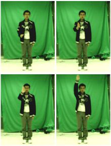
      Figure 2. Examples of sparse codes using dictionaries learned by different approaches for two action sequences from the Keck gesture
      dataset. Each waveform indicates the average of absolute sparse codes for each action sequence. The first and second row correspond
      to gesture 6 from person 2 and person 3 respectively. (a) are sample images from these sequences. Each color from the color bar in (b)
      represents one dominating class of the class distributions for dictionary items. The black dashed lines demonstrate that the curves are
      highly peaked in one class. The figure is best viewed in color and 600% zoom in.
      F (A ∪ {a1 , a2 }) − F (A ∪ {a2 }), for all A ⊆ E and                                                                                                                                                                                                                                                     denotes expectation over all pairwise distances, as in [28].
      a1 , a2 ∈ E\A. This property is referred to as diminish-                                                                                                                                                                                                                                                      Our aim is to select a subset A of E (A ⊆ E) result-
      ing returns, stating that adding an element to a smaller set                                                                                                                                                                                                                                              ing in graph G = (V, A) consisting of K connected com-
      helps more than adding it to a larger set.                                                                                                                                                                                                                                                                ponents. In addition, each vertex vi of G has a self-loop
          Matroid: [3] Let E be a finite set and I a collection of                                                                                                                                                                                                                                              ei,i . These self-loops are necessary for the proposed ran-
      subsets of E. A matroid is an ordered pair M = (E, I)                                                                                                                                                                                                                                                     dom walk model, although they do not affect graph parti-
      satisfying three conditions: (a) ∅ ∈ I; (b) If A ⊆ B and                                                                                                                                                                                                                                                  tioning. When an edge ei,j is not included in A, its weight
      B ∈ I, then A ∈ I; (c) If A ∈ I, B ∈ I and |A| < |B|,                                                                                                                                                                                                                                                     wi,j is redistributed to the self-loops of vi and vj . The edge
      then there is an element x ∈ B − A such that A ∪ x ∈ I.                                                                                                                                                                                                                                                   weights wi,i and wj,j of the self-loops are then given by:
      3.2. Graph Construction                                                                                                                                                                                                                                                                                   wi,i = wi,i + wi,j , wj,j = wj,j + wi,j . This keeps the
                                                                                                                                                                                                                                                                                                                total incident weight for each vertex constant, so that the
         We map a dataset Y into an undirected k-nearest-                                                                                                                                                                                                                                                       distribution µ in (3), below, for the graph is stationary.
      neighbor graph G = (V, E), where vertex set V denotes
      the data points, and edge set E models the pairwise relation-                                                                                                                                                                                                                                             3.3. Entropy Rate of A Random Walk
      ships between data points. Let vi be the i-th vertex and ei,j                                                                                                                                                                                                                                                We use the entropy rate of the random walk to ob-
      be an edge that connects vi and vj . The similarity between                                                                                                                                                                                                                                               tain compact and homogeneous clusters so that the con-
      vertices is given by a weight function w : E → R+ ∪ {0}.                                                                                                                                                                                                                                                  structed dictionary has good representative power. The en-
      The edge weighs are symmetric for an undirected graph,                                                                                                                                                                                                                                                    tropy rate measures the uncertainty of a stochastic process
      i.e. wi,j = wj,i . We set wi,j = 0 if there is no edge join-                                                                                                                                                                                                                                              X = {Xt |t ∈ T } where T is an index set. It can be de-
      ing vi and vj . We use a Gaussian kernel to convert pairwise                                                                                                                                                                                                                                              fined as: H(X) = limt→∞ H(Xt |Xt−1 ...X1 ), which is
      distances to similarities: wi,j = exp(−βd2 (vi , vj )), where                                                                                                                                                                                                                                             the conditional entropy of the last random variable given
      d(vi , vj ) is the distance between vi and vj . The normal-                                                                                                                                                                                                                                               the past. For a stationary 1st-order Markov chain, the en-
      ization factor β is set to β = (2hd2 (vi , vj )i)−1 , where h·i                                                                                                                                                                                                                                           tropy rate is given by: H(X) =limt→∞ H(Xt |Xt−1 ) =
limt→∞ H(X2 |X1 ) = H(X2 |X1 ).
    A random walk X = {Xt |t ∈ T, Xt ∈ V } is a sequence                                           4           4
                                                                                                                                              2       2
of vertices of the graph. We use the random walk model
                                                                                                                                              2       2

from [4] with a transition Pprobability from vi to vj : Pi,j =
                                                                                                   4           4

wi,j /wi , where wi =           j:ei,j ∈E wi,j is the total incident
weight of vi , and the stationary distribution is:                                             (a) Entropy Rate = 0.03    (b) Entropy Rate = 0.43
                                        w1 w2            w|V | t
    µ = (µ1 , µ2 , ..., µ|V | )t = (         ,    , ...,      )  (3)
                                       wall wall         wall
                 P|V |                                                                                 5                                  5       5
                                                                                                   3
where wall = i=1 wi is the sum of the total weights of                                             4                                      5       5
all vertices. The entropy rate of the random    P walk in [4] is
                                                                                                           8

defined as:
          P   H(X)
                 P      =   H(X    2 |X  1 )  =    i µi H(X2 |X1 =
vi ) = − i µi j Pi,j log Pi,j . It is a sum of the entropies                                   (c) Entropy Rate = 0.22    (d) Entropy Rate = 0.24
of the transition probabilities weighted by µi .                                      Figure 3. The importance of the entropy rate for constructing a
    The proposed graph construction leaves µ in (3) un-                               dictionary with good representative power. The number next to
changed. The set functions for the transition probabilities                           the edges is a distance between vertices. Each vertex has a self
Pi,j : 2E → R with respect to A are defined as:                                       loop which is not shown. Each figure outputs six clusters shown
                                                                                      as connected components. The red dots are cluster centers. We
                             P
                                  j:ei,j ∈A wi,j
                   1−
                  
                                      wi
                                                   if i = j,                          do not show the red dots for those clusters which only contain
                       wi,j
   Pi,j (A) =                                      if i 6= j, ei,j ∈ A,     (4)
                       wi                                                            one element. By computing the entropy rate, we observe that the
                      0                            if i 6= j, ei,j ∈
                                                                   / A.
                  
                                                                                      more compact clusters in (b) are preferred compared to (a), while
   Consequently, we can define a set function for the en-                             the more symmetric cluster, that is, homogeneous cluster in (d) is
tropy rate of the random walk on G = (V, A) as:                                       preferred compared to (c). It demonstrates that the cluster centers,
                    X X                                                               i.e. dictionary items, in (b)(d) have good representative power.
        H(A) = −       µi    Pi,j (A) log(Pi,j (A)).  (5)
                              i         j
    Intuitively, given µi , maximizing the entropy rate in (5)
encourages the edges from each vi to have similar weights,
i.e., similar transition probabilities to its connected vertices.
Similarly, given the entropies of transition probabilities,
                                                                                  (a) Disc. Fun. = −2.00 (b) Disc. Fun. = −1.33 (c) Disc. Fun. = −1.00
maximizing the entropy rate in (5) encourages the edges
from vi which have large weight (small distance) to be se-                            Figure 4. The importance of the discriminative term for construct-
lected. Hence the entropy rate of the random walk on the                              ing a dictionary with discriminative capabilities. The colors of
graph can generate compact and homogeneous clusters, as                               empty circles denote different categories of data points. The con-
                                                                                      nected components show different clusters. The red dots in the
shown in Figure 3. It results in dictionary items that repre-
                                                                                      figure are cluster centers. The green and black points in (b) are
sent the input signals well.                                                          grouped into the same word and consequently cannot be distin-
    The entropy rate of a random walk H : 2E → R on the                               guished. The green points in (a) are separated into two words and
proposed constructed graph is a monotonically increasing                              as a result the sparse representations for other green points might
and submodular function. Monotonicity is obvious because                              not be similar. The more ‘class pure’ clustering in (c) has a higher
the addition of any edge to A increases the uncertainty of a                          objective value than (b). The fewer number of clusters in (c) has
jump in a random walk. Submodularity is related to the ob-                            a higher objective value than (a). Sparse codes obtained by the
servations that the increase of the uncertainty from selecting                        cluster centers in (c) are best for classification. Hence the dis-
an edge ei,j is less in a later stage because it will be shared                       criminative term suggests the higher discriminative power for the
with more edges connected to vi or vj [19]. The proof is                              cluster centers in (c).
given in the supplementary material based on [19].                                       Let NA denote the number of connected components
3.4. Discriminative Function                                                          or subgraphs. The graph partitioning for A is SA =
    We construct a discriminative function that encourages                            {S1 ...SNA }. The class purity for cluster Si is computed
the sparse representations of signals over learned dictionary                         as: P(Si ) = C1i maxy Nyi , where y denotes the class label,
                                                                                      y ∈ {1...m}, and Ci = y Nyi is the total count for objects
                                                                                                              P
(i.e. cluster centers), from the same class to be similar.
    Let m denote the number of object categories. N =                                 of all classes assigned
                                                                                                            Pto cluster i. ThusPthe overall purity
                                                                                                              NA Ci              NA 1            i
[N1 ...NN ] ∈ Rm×N is a count matrix for the number of                                for SA is:P(SPA  ) =    i=1 C P(Si ) =     i=1 C maxy Ny ,
elements from each object class assigned to each cluster 1 .                          where C = i Ci . The discriminative term is defined as:
                                                                                                                    NA
Let Ni = [N1i ...Nm  i t
                       ] , where Nmi
                                     is the number of objects                                                       X     1
from the m-th class that were assigned to the i-th cluster.                               Q(A) ≡ P(SA ) − NA =              max Nyi − NA . (6)
                                                                                                                    i=1
                                                                                                                         C   y
   1 each   input signal can be considered as an individual cluster here.                The purity term P(SA ) encourages clusters with pure
class labels, while NA favors a smaller number of clusters.         Note that the edges that induce cycles in the graph have
The class pure cluster encourages similar feature points to      no effect on the graph partition. In order to speed up the op-
be represented by the same cluster centers (i.e., dictionary     timization, a cycle-free constraint is used here so that those
items). Hence, it should result in high discrimination power     edges are not included in A. This greatly reduces the eval-
for the dictionary items. From Figure 4, the more class          uations in the greedy search and leads to a smaller solution
pure cluster is preferred for a fixed number of clusters,        space. The cycle-free constraint and the connected compo-
while a fewer number of clusters is preferred for a fixed        nent constraint in the graph partitioning, i.e. NA ≥ K in-
purity. Similar to the entropy rate, the discriminative term     duce a matroid M = (E, I). I is the collection of subsets
Q : 2E → R, is also a monotonically increasing and sub-          A ⊆ E which satisfies: A includes no cycles and the graph
modular function.                                                partition from A has more than K connected components.
   The final objective function combines the entropy rate           Maximization of a submodular function with a matroid
and the discriminative term for dictionary learning, i.e.,       constraint gives a 1/2-approximation bound on the opti-
F (A) ≡ H(A) + λQ(A). The solution is achieved by max-           mality of the solution [24]. Hence the greedy algorithm
imizing the objective function with A selected as:               can obtain a performance-guaranteed solution. Algorithm
   max H(A) + λQ(A) s.t. A ⊆ E and NA ≥ K,                (7)    1 presents the pseudocode of our algorithm.
     A
                                                                 3.6. Algorithm Complexity
where λ controls the relative contribution between entropy
rate and the discriminative term. NA ≥ K is a constraint            The complexity of a naive implementation of Algorithm
on the number of connected components. This constraint           1 is O(|V |2 ), because it iterates O(|V |) times to select
enforces exactly K connected components because the ob-          edges, and evaluates the whole edge list to select the edge
jective function                              λ is given by      which has the largest gain at each iteration. Actually we can
               is monotonically increasing.
                                H(ei,j )−H(∅)
                     maxe                                        further exploit the submodularity property of the objective
                                   
λ = γλ0 = maxei,j Q(ei,j )−Q(∅) λ0 , where λ0 is a pre-
                     i,j                                         function to speed up the optimization.
defined parameter and γ is the ratio of maximal entropy
                                                                    We first evaluate the gain in the objective function for
rate increase and the maximal discriminative term increase
                                                                 each edge and construct a max heap structure. The edge
when adding a single edge to the graph.
                                                                 with the largest gain is selected as the top element from the
   The objective function in (7) is submodular and mono-         heap at each iteration. The addition of any edge into A im-
tonically increasing, because it is a linear combination of      pacts the gains of the remaining edges. Here, instead of re-
monotonic and submodular functions [24]. This makes the          computing the gains for every remaining edge in the heap,
clusters more compact and class pure. Their cluster centers
                                                                 we perform lazy evaluation which only updates the gain of
represent the input signals well and preserve object cate-       the top element. The key idea is to realize that the gain for
gory information. Hence when using these cluster centers         each edge can never increase because of the diminishing re-
as dictionary items, our approach encourages the computed
                                                                 turn property. In many cases, the recomputation of gain for
sparse codes for signals from the same class to be similar,      the top element is not much smaller, hence the top element
as shown in Figures 1(b) and 2(b).                               will stay the top element even after the update.
                                                                    The worst case is that we need to update the gain for
Algorithm 1 Submodular Dictionary Learning (SDL)
                                                                 each edge and then re-establish the heap property after the
 Input: G = (V, E), w, K, λ and N
 Output: D                                                       addition of any edge into A. That is, we need to rebuild
 Initialization: A ← ∅, D ← ∅                                    the heap, which takes O(|V | log |V |) time, hence the worse
 for NA > K do
    ẽ = argmax F (A ∪ {e}) − F (A)                              case is O(|V |2 log |V |) [3]. In fact, only a few updates are
           A∪{e}∈I
   A ← A ∪ {ẽ}
                                                                 ever performed in the heap at each iteration, hence the com-
 end for                                                         plexity of our algorithm is effectively O(|V | log |V |) 2 .
                      in G = (V, A) do
 for each subgraph Si P
   D ← D ∪ { |S1 |       j:v ∈S vj }
                     i      j     i                              4. Classification Approach
 end for
                                                                 4.1. Face and Object Recognition
3.5. Optimization                                                   Our dictionary learning algorithm forces the signals from
   Direct maximization of a submodular function is a NP-         the same class to have very similar sparse representations,
hard problem. However, one simple approximate solution           which results in good classification performance even using
can be obtained by a greedy algorithm from [24]. The al-         a simple linear classifier. For face and object recognition in
gorithm starts from a empty set A = ∅ and iteratively adds       static images, we employ the multivariate ridge regression
edges to A. It always chooses the edge which provides the
largest gain for F at each iteration. The iterations stop when       2 The complexity here does not include the complexity of constructing

the desired number of connected components is obtained.          the k-nearest-neighbor graph G, which is an input to our algorithm.
model with the quadratic loss and L2 norm regularization:                                          Table 1. Computation time (s) for dictionary training using
                                                                                                   random-face features on the Extended YaleB database.
        W = arg min ||H − W Z||2 + α||W ||22 ,         (8)                                              Dict. size                 418           456          494                                532      570              608        646        684
                        W
                 m×K                                                                                      SDL                       0.9          1.0           0.9                                0.9     0.9               1.0       0.9        0.9
where W ∈ R           denotes the linear classifier parameters                                         K-SVD [1]                   52.6          56.1         59.8                               64.9     67.9             72.2       76.2      78.0
and H = [h1 ...hN ] ∈ Rm×N are the class label matrix of                                              D-KSVD [35]                  53.1          56.9         60.5                               65.8     68.1             74.9       77.6      79.2
                                                                                                      LC-KSVD [12]                 67.2          72.6         78.3                               86.5     90.7             97.8      104.4      112.3
input signals Y . hi = [0, 0...1...0, 0]t ∈ Rm is a label vec-
tor corresponding to an input signal yi , where the non-zero                                       0.96
                                                                                                                                                                                        0.75

position indicates the class of yi . (8) yields the solutions:                                     0.94
                                                                                                                                                                                         0.7

                                                                         Classification Accuracy

                                                                                                                                                              Classification Accuracy
W = (ZZ t + αI)−1 ZH t .                                                                           0.92                                                                                 0.65

    For a test image yi , we first compute its sparse represen-                                     0.9

                                                                                                   0.88
                                                                                                                                    SDL
                                                                                                                                    baseline
                                                                                                                                                                                         0.6

                                                                                                                                    KSVD

tation zi using (1). Then we simply use W in (8) obtained                                          0.86
                                                                                                                                    DKSVD
                                                                                                                                    LCKSVD
                                                                                                                                                                                        0.55
                                                                                                                                                                                                                SDL
                                                                                                                                                                                                                baseline
                                                                                                                                    SRC
from training data to estimate a class label vector: l = W zi ,                                    0.84                             LLC
                                                                                                                                                                                         0.5                    KSVD
                                                                                                                                                                                                                DKSVD
                                                                                                                                                                                                                LCKSVD

where l ∈ Rm . The label of yi is the index i where li is the
                                                                                                   0.82                                                                                 0.45
                                                                                                                                                                                                                SRC
                                                                                                                                                                                                                LLC
                                                                                                    0.8
                                                                                                                                                                                         0.4

largest element of l.                                                                                380   418   456   494   532    570
                                                                                                                       Dictionary Size
                                                                                                                                           608    646   684                                306    510   714     918
                                                                                                                                                                                                          Dictionary Size
                                                                                                                                                                                                                           1122   1326   1530

                                                                                                                                                  0
                                                                                                   (a) Extended YaleB, k = 1, λ = 1                                                        (b) Caltech101, k = 10, λ0 = 1
4.2. Action Classification
                                                                                                   Figure 5. Classification accuracy performances using different ap-
   For the classification of action sequences, we first com-                                       proaches with different dictionary sizes. (a) Performance on the
pute the sparse representations for each frame, then employ                                        Extended YaleB; (b) Performance on the Caltech101.
dynamic time warping (DTW) to align and measure the dis-
tance between two sequences in the sparse representation                                           sification accuracy is 95.9% when SRC directly uses all
domain; next a K-NN classifier is used for recognition.                                            the training data as the dictionary (The result of our ap-
                                                                                                   proach is 96.4%, which only shows that the linear classi-
5. Experiments                                                                                     fier in (8) used in SDL is slightly better than reconstruction
   We evaluate our approach on the Extended YaleB                                                  error based classifier used in SRC).
database [8], Caltech101 [6] and Keck gesture dataset [17].                                            In Figure 6(a), we plot the performance curves for a
We compare our results with K-SVD [1], D-KSVD [35],                                                range of λ0 for a fixed k = 1 (recall k is the number of
LC-KSVD [12], SRC [30], and LLC [29] for learning a                                                nearest neighbors used to construct the original graph). We
dictionary directly from the training data on the Extended                                         observe that our approach is insensitive to the selection of
YaleB and Caltech101 dataset, while we compare our re-                                             λ0 . Hence we use λ0 = 1.0 throughout the experiments.
sults with K-means, Liu-Shah [18], MMI [26] and ME [10]                                            Figure 6(b) shows the performance curves for a range of k
for learning a dictionary from a large set of dictionary item                                      for λ0 = 1.0. We observe that a smaller value of k results in
candidates on the Keck gesture dataset. The baseline ap-                                           better performances. This also leads to more efficient dic-
proach is to replace our discriminative function with a bal-                                       tionary learning since the size of the heap is proportional to
ance function described in [19], which aims to balance the                                         the size of the edge set of G.
size of each cluster. We refer to it and our approach as ‘base-                                        We also compare the computation time of training a dic-
line’ and ‘SDL’, respectively, in the following.                                                   tionary with K-SVD, D-KSVD and LC-KSVD. The param-
5.1. Dictionary Learning from the Training Data                                                    eter k is set to 1 since we get good performance in Fig-
5.1.1 Extended YaleB Database                                                                      ure 6(b). In Table 1, our approach is at least 50 times faster
                                                                                                   than the state of art dictionary learning approaches.
The Extended YaleB database contains 2, 414 frontal face
images of 38 persons [8]. There are 64 images with a size                                          5.1.2 Caltech101 Dataset
of 192 × 168 pixels for each person. This dataset is chal-                                         The Caltech101 dataset [6] contains 9144 images from 102
lenging due to varying illuminations and expressions. We                                           classes (i.e. 101 object classes and a ‘background’ class).
randomly select half of the images as training and the other                                       The samples from each class have significant shape dif-
half for testing. Following the setting in [35], each face is                                      ferences. Following [12], we extract spatial pyramid fea-
represented as a 504 sized random-face feature vector.                                             tures [15] for each image and then reduce them to 3000
    We evaluate our approach in terms of the classification                                        dimensions by PCA. The sparse codes are computed from
accuracy using dictionary sizes 380 to 684, and compare                                            spatial pyramid features. Following the common experi-
it with baseline, K-SVD [1], D-KSVD [35], SRC 3 [30],                                              mental protocol, we train on randomly selected 5, 10, 15,
LLC [29] and the recently proposed LC-KSVD [12]. The                                               20, 25 and 30 samples per category and test on the rest. We
sparsity s is set to 30. Figure 5(a) shows that our approach                                       repeat the experiments 10 times and the final results are re-
outperforms the state of the art approaches in terms of clas-                                      ported as the average and standard deviation of each run.
sification accuracy with different dictionary sizes. The clas-                                        We evaluate our approach and compare the results with
   3 We randomly choose the average of dictionary size per person from                             state-of-art approaches [30, 1, 35, 12, 34, 15, 9, 2, 11, 25,
each person and report the best performance achieved.                                              7, 31, 29]. The sparsity s is set to 30. The comparative
0.96

                          0.955
                                                                                                                    0.95                                                            Table 3. Computation time (s) for dictionary training using spatial
                           0.95
Classification Accuracy

                                                                                          Classification Accuracy
                          0.945                                                                                     0.94                                                            pyramid features on the Caltech101 dataset.
                           0.94
                                                                                                                    0.93                                                               Dict. size      306       510       714     918    1122   1326    1530
                          0.935
                                                                                                                    0.92
                                                                                                                                                                                         SDL           37.5     36.7      36.6    36.9    37.1   36.7    36.7
                           0.93

                          0.925
                                                                         λ’=0.008
                                                                         λ’=0.02
                                                                                                                                                                       k=1            K-SVD [1]       578.3     790.1     1055    1337    1665   2110    2467
                                                                                                                    0.91                                               k=2
                           0.92                                          λ’=0.05                                                                                       k=5           D-KSVD [35]      560.1     801.3     1061    1355    1696   2081    2551
                                                                         λ’=0.1                                                                                        k=15
                          0.915
                                                                         λ’=1.0
                                                                                                                     0.9
                                                                                                                                                                       k=30
                                                                                                                                                                                     LC-KSVD [12]     612.1     880.6     1182    1543    1971   2496    3112
                           0.91                                                                                     0.89
                              380    418   456   494   532   570   608     646      684                                380   418   456    494    532   570       608   646    684
                                                 Dictionary Size                                                                          Dictionary Size
                                                         0
                                     (a) Varying λ for k = 1                                                                 (b) Varying k for λ = 1         0                      Table 4. Computation time (s) for dictionary training using shape
                           Figure 6. Effects of parameter selection of λ0 and k on the classi-                                                                                      features on the Keck gesture dataset.
                           fication accuracy performance on the Extended YaleB database.                                                                                               Dict. size     40       60         80      100     120     140     160    180
                                                                                                                                                                                         SDL         1.0       1.0       1.1      1.0     1.0     1.1     1.0    1.0
                           Table 2. Classification accuracies using spatial pyramid features                                                                                           K-means       1.2       1.1       1.6      1.4     1.8     2.1     2.1    2.2
                                                                                                                                                                                       ME [10]       48.5     57.2       70.2    84.6    91.5    113.1   118.9   130
                           on the Caltech101. SDL also provides the standard deviations.                                                                                             LiuShah [18]   599.2     597.9     597.2    596.1   593.9   590.3   587.4   582
                                    Training Images              5                 10                                        15           20            25                 30         MMI [26]       64.6     92.6      115.5    140.3   150.1   164.1   184.4   201
                                      Malik [34]               46.6               55.8                                      59.1         62.0            -               66.20
                                     Lazebnik [15]               -                  -                                       56.4           -             -                64.6
                                       Griffin [9]             44.2               54.5                                      59.0         63.3          65.8              67.60
                                                                                                                                                                                    code motion information. Both types of feature descriptor
                                        Irani [2]                -                  -                                       65.0           -             -               70.40      are 256 dimensions. We compute the class distribution ma-
                                     Grauman [11]                -                  -                                       61.0           -             -               69.10
                                    Venkatesh [25]               -                  -                                       42.0           -             -                  -
                                                                                                                                                                                    trix introduced in [26] to obtain the count matrix N .
                                      Gemert [7]                 -                  -                                         -            -             -               64.16          Following the experimental settings in [26], we obtain an
                                       Yang [31]                 -                  -                                       67.0           -             -               73.20
                                       Wang [29]               51.15             59.77                                     65.43         67.74         70.16             73.44
                                                                                                                                                                                    initial large dictionary D0 via K-SVD. The dictionary size
                                       SRC [30]                48.8               60.1                                      64.9         67.7          69.2               70.7      |D0 | is set to be approximately twice the dimension of the
                                      K-SVD [1]                49.8               59.8                                      65.2         68.7          71.0               73.2
                                     D-KSVD [35]               49.6               59.5                                      65.1         68.6          71.1               73.0
                                                                                                                                                                                    feature descriptor. Given D0 , our aim is to learn a compact
                                    LC-KSVD [12]               54.0               63.1                                      67.7         70.5          72.3               73.6      and discriminative dictionary D∗ .
                                                               55.3               63.4                                      67.5         70.7          73.1               75.3
                                           SDL
                                                               ±0.5              ± 0.5                                     ± 0.3         ± 0.3         ± 0.4             ± 0.4
                                                                                                                                                                                        We employ a leave-one-person-out protocol to report the
                                                                                                                                                                                    classification result. A sparsity value of 30 is used. We eval-
                           results are shown in Table 2. Our approach outperforms all                                                                                               uate our approach with different dictionary sizes and differ-
                           the competing approaches except the comparison with LC-                                                                                                  ent features. Then we compare our results with the base-
                           KSVD in the case of 15 training samples per category.                                                                                                    line, K-means, and Liu-Shah [18], ME [10] and MMI [26].
                              We randomly select 30 images per category as training                                                                                                 In Figure 7, our results outperform the baseline, K-means,
                           images, and evaluate our approach with different dictionary                                                                                              Liu-Shah, ME and MMI, and is comparable to MMI* 5 .
                           sizes from 306 to 1530. We also compare our results with                                                                                                     To evaluate the discrimination and compactness of
                           the baseline, K-SVD [1], D-KSVD [35], LC-KSVD [12],                                                                                                      learned dictionaries, we learned a 40 element dictionary
                           SRC [30] and LLC [29]. Figure 5(b) shows that our ap-                                                                                                    from D0 using six different approaches. Purity is the his-
                           proach outperforms the competing K-SVD, D-KSVD, SRC,                                                                                                     togram of maximum probabilities of observing any class
                           LLC and is comparable to LC-KSVD.                                                                                                                        given a dictionary item [14]. Compactness is captured by
                              We also compare the computation time of training a dic-                                                                                               the histogram of pairwise correlation coefficients of items
                           tionary with the K-SVD, D-KSVD and LC-KSVD. The pa-                                                                                                      in D∗ [35] (lower correlations better). From Figure 8, our
                           rameter k (for k-nearest-neighbor graph construction) is 10.                                                                                             approach is most pure, and second most compact compared
                           As shown in Table 3, our approach can train approximately                                                                                                to the baseline, K-means, and Liu-Shah, ME and MMI.
                           15 times faster when we construct a dictionary of size 306.                                                                                                  In addition, we compare the computation time to learn
                           More importantly, our approach does not degrade too much                                                                                                 a dictionary using shape features with K-means, Liu-Shah,
                           even with a dictionary of size 1530. The computation time                                                                                                ME and MMI. The parameter k is set to 3. Our approach is
                           for learning a dictionary using these state-of-art approaches                                                                                            at least 50 times faster than Liu-Shah, ME and MMI in Ta-
                           increases with the dictionary size; however, the computa-                                                                                                ble 4. The computation time using K-means is comparable
                           tion time for our approach remains nearly constant.                                                                                                      to our approach, but its classification accuracy performance
                           5.2. Dictionary Learning from A Large Set of Dic-                                                                                                        is much poorer than ours, as shown in Figure 7.
                                 tionary Item Candidates                                                                                                                            6. Conclusion
                           5.2.1 Keck Gesture Dataset                                                                                                                                  We present a greedy-based dictionary learning approach
                           The Keck gesture dataset [17] consists of 14 different ges-                                                                                              via maximizing a monotonically increasing and submod-
                           tures 4 , which are a subset of the military signals. We use                                                                                             ular function. By integrating the entropy rate of a ran-
                           the silhouette-based descriptor from [17] to capture shape                                                                                               dom walk on a graph and a discriminative term into the
                           information while we use optical-flow based features to en-
                                                                                                                                                                                       5 MMI   and MMI* here are the MMI1 and MMI2 approaches in [26]
                                    4 The gesture
                                             classes include turn left, turn right, attention left, attention                                                                       respectively. K-means, ME and MMI results are based on our own imple-
                           right, flap, stop left, stop right, stop both, attention both, start, go back,                                                                           mentations while MMI* results are copied from the original paper. For the
                           close distance, speed up and come near.                                                                                                                  K-means method, we perform K-means clustering over D 0 to obtain D ∗ .
1

                                                                                                                                                                     0.95                                                                                                  0.95
                                                      0.9

                            Classification Accuracy

                                                                                                                                           Classification Accuracy

                                                                                                                                                                                                                                                 Classification Accuracy
                                                                                                                                                                      0.9                                                                                                   0.9
                                                      0.8

                                                                                                                                                                     0.85                                                                                                  0.85
                                                      0.7

                                                                                                                                                                      0.8                                                                                                   0.8
                                                      0.6

                                                                     SDL                                                                                                              SDL                                                                                                SDL
                                                                                                                                                                     0.75                                                                                                  0.75
                                                      0.5                                                                                                                             baseline                                                                                           baseline
                                                                     baseline
                                                                     K−means                                                                                                          K−means                                                                                            K−means
                                                      0.4                                                                                                             0.7             ME                                                                                    0.7          ME
                                                                     ME
                                                                     Liu−Shah                                                                                                         Liu−Shah                                                                                           Liu−Shah
                                                      0.3            MMI                                                                                             0.65             MMI                                                                                  0.65          MMI
                                                                     MMI*                                                                                                             MMI*                                                                                               MMI*
                                                      0.2                                                                                                             0.6                                                                                                   0.6
                                                         20         40     60       80      100    120     140   160     180   200                                       20      40       60     80      100   120      140   160   180   200                                  20   40       60     80      100   120      140   160   180   200
                                                                                         Dictionary Size                                                                                              Dictionary Size                                                                                    Dictionary Size
                                                                                            0                                                                                                             0                                                                                                        0
                                                            (a) Shape, |D | = 600, k = 3                                                                                (b) Motion, |D | = 600, k = 6                                           (c) Shape + Motion, |D | = 1200, k = 2
Figure 7. Classification accuracy using different approaches with different features and dictionary sizes. The results for MMI* are copied
from [26]. The classification accuracy using initial dictionary D0 : (1) 26% (shape); (2) 26% (motion); (3) 36% (joint shape-motion).
600                                                                                               40
                                                                         SDL                                                                                                  SDL
500
                                                                         baseline                 35                                                                          baseline                                [9] G. Griffin, A. Holub, and P. Perona. Caltech-256 object category dataset, 2007.
                                                                         K−means                                                                                              K−means
                                                                         ME                       30                                                                          ME                                          CIT Technical Report 7694.
                                                                         Liu−Shah                                                                                             Liu−Shah
400
                                                                         MMI                      25                                                                          MMI                                    [10] C. Guestrin, A. Krause, and A. Singh. Near-optimal sensor placements in gaus-
300                                                                                               20
                                                                                                                                                                                                                          sian processes, 2005. ICML.
200
                                                                                                  15                                                                                                                 [11] P. Jain, B. Kullis, and K. Grauman. Fast image search for learned metrics, 2008.
                                                                                                  10
                                                                                                                                                                                                                          CVPR.
100
                                                                                                   5                                                                                                                 [12] Z. Jiang, Z. Lin, and L. Davis. Learning a discriminative dictionary for sparse
  0                                                                                                0
                                                                                                                                                                                                                          coding via label consistent k-svd, 2011. CVPR.
         0.2   0.4    0.6                                     0.8           1                            0.2           0.4           0.6    0.8                                  1

      (a) Compactness,|D ∗ | = 40                                                                              (b) Purity, |D ∗ | = 40                                                                               [13] A. Krause and V. Cevher. Submodular dictionary selection for sparse represen-
                                                                                                                                                                                                                          tation, 2010. ICML.
Figure 8. Purity and compactness comparisons with dictionary size                                                                                                                                                    [14] S. Lazebnik and M. Raginsky. Supervised learning of quantizer codebooks by
40 on the Keck gesture dataset. At the left-most bin of (a) and                                                                                                                                                           information loss minimization. TPAMI, 31(7):1294–1309, 2009.
the right-most bin of (b), a compact and discriminative dictionary                                                                                                                                                   [15] S. Lazebnik, C. Schmid, and J. Ponce. Beyond bags of features: Spatial pyra-
should have high purity and high compactness.                                                                                                                                                                             mid matching for recognizing natural scene categories, 2007. CVPR.
                                                                                                                                                                                                                     [16] H. Lee, A. Battle, R. Raina, and A. Y. Ng. Efficient sparse coding algorithms,
objective function, which makes each cluster compact and                                                                                                                                                                  2006. NIPS.
                                                                                                                                                                                                                     [17] Z. Lin, Z. Jiang, and L. Davis. Recognizing actions by shape-motion prototypes
class pure, the learned dictionary is both representative and                                                                                                                                                             trees, 2009. ICCV.
discriminative. The objective function is optimized by a                                                                                                                                                             [18] J. Liu and M. Shah. Learning human actions via information maximization,
highly efficient greedy algorithm, which can be easily ap-                                                                                                                                                                2008. CVPR.
                                                                                                                                                                                                                     [19] M. Liu, O. Tuzel, S. Ramalingam, and R. Chellappa. Entropy rate superpixel
plied to a large dataset. It outperforms recently proposed                                                                                                                                                                segmentation, 2011. CVPR.
dictionary learning approaches including D-KSVD [35],                                                                                                                                                                [20] J. Mairal, F. Bach, J. Ponce, G. Sapiro, and A. Zisserman. Discriminative
SRC [30], LLC [29], Liu-Shah [18], ME [10], MMI [26],                                                                                                                                                                     learned dictionaries for local image analysis, 2008. CVPR.
                                                                                                                                                                                                                     [21] J. Mairal, F. Bach, J. Ponce, G. Sapiro, and A. Zisserman. Supervised dictionary
and can be comparable to LC-KSVD [12]. Possible future                                                                                                                                                                    learning, 2009. NIPS.
work includes exploring methods for efficiently updating                                                                                                                                                             [22] J. Marial, F. Bach, J. Ponce, and G. Sapiro. Online dictionary learning for
the learned dictionary for a new category while keeping its                                                                                                                                                               sparse coding, 2009. ICML.
                                                                                                                                                                                                                     [23] M. Narasimhan, N. Jojic, and J. Bilmes. Q-clustering, 2005. NIPS.
the representative and discriminative power.
                                                                                                                                                                                                                     [24] G. Nemhauser, L. Wolsey, and M. Fisher. An analysis of the approximations
                                                                                                                                                                                                                          for maximizing submodular set functions. Mathematical Programming, 1978.
Acknowledgement
                                                                                                                                                                                                                     [25] D. Pham and S. Venkatesh. Joint learning and dictionary construction for pat-
   This work was supported by the Army Research Of-                                                                                                                                                                       tern recognition, 2008. CVPR.
fice MURI Grant W911NF-09-1-0383 and the Global                                                                                                                                                                      [26] Q. Qiu, Z. Jiang, and R. Chellappa. Sparse dictionary-based representation and
                                                                                                                                                                                                                          recognition of action attributes, 2011. ICCV.
Land Cover Facility with NASA Grants NNX08AP33A,                                                                                                                                                                     [27] F. Rodriguez and G. Sapiro. Sparse representations for image classification:
NNX08AN72G and NNX11AH67G.                                                                                                                                                                                                Learning discriminative and reconstructive non-parametric dictionaries.
                                                                                                                                                                                                                     [28] C. Rother, V. Kolmogorov, and A. Blake. Interactive foreground extraction
References                                                                                                                                                                                                                using iterated graph cuts, 2004. SIGGRAPH.
      [1] M. Aharon, M. Elad, and A. Bruckstein. K-svd: An algorithm for designing                                                                                                                                   [29] J. Wang, J. Yang, K. Yu, F. Lv, T. huang, and Y. Gong. Locality-constrained
          overcomplete dictionries for sparse representation. IEEE Trans. on Signal Pro-                                                                                                                                  linear coding for image classification, 2010. CVPR.
          cessing, 54(1):4311–4322, 2006.                                                                                                                                                                            [30] J. Wright, M. Yang, A. Ganesh, S. Sastry, and Y. Ma. Robust face recognition
      [2] O. Boiman, E. Shechtman, and M. Irani. In defense of nearest-neighor based                                                                                                                                      via sparse representation. TPAMI, 31(2):210–227, 2009.
          image classification, 2008. CVPR.                                                                                                                                                                          [31] J. Yang, K. Yu, Y. Gong, and T. Huang. Linear spatial pyramid matching using
      [3] T. Cormen, C. Leiserson, R. Rivest, and C. Stein. Introduction to Algorithms,                                                                                                                                   sparse coding for image classification, 2009. CVPR.
          3rd Edition, 2009.                                                                                                                                                                                         [32] J. Yang, K. Yu, and T. Huang. Supervised translation-invariant sparse coding,
      [4] T. Cover and J. Thomas. Elements of Information Theory, 2nd Edition, 2006.                                                                                                                                      2010. CVPR.
                                                                                                                                                                                                                     [33] L. Yang, R. Jin, R. Sukthankar, and F. Jurie. Unifying discriminative visual
      [5] K. Engan, S. Aase, and J. Husφy. Frame based signal compression using
                                                                                                                                                                                                                          codebook genearation with classifier training for object category recognition,
          method of optimal directions (mod), 1999. IEEE Symp. Circ. Syst.
                                                                                                                                                                                                                          2008. CVPR.
      [6] L. FeiFei, R. Fergus, and P. Perona. Learning generative visual models from                                                                                                                                [34] H. Zhang, A. Berg, M. Maire, and J. Malik. Svm-knn: Discriminative nearest
          few training samples, 2004. CVPR Workshop.                                                                                                                                                                      neighbor classification for visual category recognition, 2006. CVPR.
      [7] J. Gemert, J. Geusebroek, C. Veenman, and A. Smeulders. Kernel codebooks                                                                                                                                   [35] Q. Zhang and B. Li. Discriminative k-svd for dictionary learning in face recog-
          for scene categorization, 2008. ECCV.                                                                                                                                                                           nition, 2010. CVPR.
      [8] A. Georghiades, P. Belhumeur, and D. Kriegman. Illumination cone models                                                                                                                                    [36] L. Zhao, H. Nagamochi, and T. Ibaraki. Greedy splitting algorithms for approx-
          for face recognition under variable lighting and pose. TPAMI, 23(6):643–660,                                                                                                                                    imating multiway partition problems. Mathematical Programming, 2005.
          2001.
You can also read