Transverse momentum dependent parton densities in a proton from the generalized DAS approach - Inspire HEP
←
→
Page content transcription
If your browser does not render page correctly, please read the page content below
Published for SISSA by         Springer
                                                                    Received: November 8, 2019
                                                                    Accepted: January 20, 2020
                                                                    Published: February 4, 2020

Transverse momentum dependent parton densities in

                                                                                                  JHEP02(2020)028
a proton from the generalized DAS approach

A.V. Kotikov,a,b A.V. Lipatov,b,c B.G. Shaikhatdenovb and P. Zhangd
a
  Institute of Modern Physics,
  Lanzhou 730000, China
b
  Joint Institute for Nuclear Research,
  141980, Dubna, Moscow region, Russia
c
  Skobeltsyn Institute of Nuclear Physics, Lomonosov Moscow State University,
  119991, Moscow, Russia
d
  School of Physics and Astronomy, Sun Yat-sen University,
  Zhuhai 519082, China
    E-mail: kotikov@theor.jinr.ru, lipatov@theory.sinp.msu.ru,
    binur1@yahoo.com, zhangpm5@mail.sysu.edu.cn

Abstract: We use the Bessel-inspired behavior of parton densities at small Bjorken x
values, obtained in the case of the flat initial conditions for DGLAP evolution equations in
the double scaling QCD approximation (DAS), to evaluate the transverse momentum de-
pendent (TMD, or unintegrated) quark and gluon distribution functions in a proton. The
calculations are performed analytically using the Kimber-Martin-Ryskin (KMR) prescrip-
tion with different implementation of kinematical constraint, reflecting the angular and
strong ordering conditions. The relations between the differential and integral formulation
of the KMR approach is discussed. Several phenomenological applications of the proposed
TMD parton densities to the LHC processes are given.

Keywords: QCD Phenomenology

ArXiv ePrint: 1911.01445

Open Access, c The Authors.
                                                     https://doi.org/10.1007/JHEP02(2020)028
Article funded by SCOAP3 .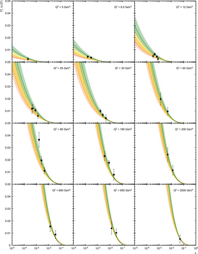
Contents

1 Introduction                                                                           1

2 Theoretical framework                                                                  3
  2.1 PDFs and proton structure function F2 (x, Q2 )                                     3
  2.2 Kimber-Martin-Ryskin approach                                                      5

3 Calculations                                                                           6

                                                                                              JHEP02(2020)028
  3.1 Sudakov form factors Ta (µ2 , k 2 )                                                6
  3.2 TMDs from differential formulation of KMR approach                                 6
  3.3 TMDs from integral formulation of KMR approach                                     7
  3.4 Cut-off parameter ∆                                                                8
                       (i)                 (d)
  3.5 Comparison of fa (x, k 2 , µ2 ) and fa (x, k 2 , µ2 )                              8
  3.6 Infrared modification of the strong coupling                                       9
  3.7 Beyond small x                                                                    10

4 Phenomenological applications                                                         13
  4.1 Inclusive b-jet production at the LHC                                             13
  4.2 Inclusive Higgs boson production at the LHC                                       14
  4.3 Proton structure functions F2c (x, Q2 ) and F2b (x, Q2 )                          19

5 Conclusions                                                                           20

1   Introduction

A theoretical description of a number of high energy processes at hadron colliders which
proceed with large momentum transfer and containing multiple hard scales can be obtained
with transverse momentum dependent (TMD), or unintegrated, parton (quark and/or
gluon) density functions in a proton [1]. These quantities depend on the fraction x of
the proton longitudinal momentum carried by a parton, the two-dimensional parton trans-
verse momentum k2T and hard scale µ2 of the hard process and encode non-perturbative
information on proton structure, including transverse momentum and polarization degrees
of freedom. They are related to the physical cross sections and other observables, measured
in the collider experiments, via TMD factorization theorems in Quantum Chromodynamics
(QCD). The latter provide the necessary framework to separate hard partonic physics, de-
scribed with a perturbative QCD expansion, from soft hadronic physics. At present, there
are number of factorization approaches which incorporate the transverse momentum depen-
dence in the parton distributions: for example, the Collins-Soper-Sterman approach [2, 3]
(or TMD factorization), designed for semi-inclusive processes with a finite and non-zero

                                           –1–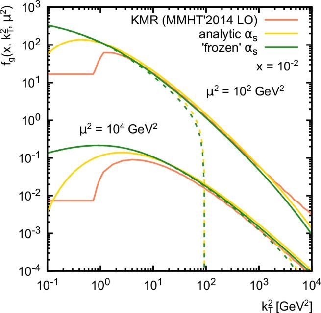
ratio between the hard scale µ2 and total energy s, and high-energy factorization [4, 5] (or
kT -factorization [6, 7]) approach, valid in the limit of a fixed hard scale and high energy.
     In the high-energy factorization, the TMD gluon density satisfies the Balitsky-Fadin-
Kuraev-Lipatov (BFKL) [8–10] or Ciafaloni-Catani-Fiorani-Marchesini (CCFM) [11–14]
evolution equations, which resum large terms proportional to αsn lnn s ∼ αsn lnn 1/x, impor-
tant at high energies s (or, equivalently, at small x). Thus, one can effectively take into
account higher-order radiative corrections to the production cross sections (namely, a part
of NLO + NNLO +. . . terms corresponding to the initial-state real gluon emissions). The
CCFM equation takes into account additional terms proportional to αsn lnn 1/(1 − x) and
therefore is valid at both small and large x. The number of phenomenological applications

                                                                                                JHEP02(2020)028
of the high-energy factorization and CCFM evolution is known in the literature (see, for
example, [15–25] and references therein).
     There are also other approaches determining the TMD gluon and quark density func-
tions in a proton. So, one can evaluate them using the schemes based on the conventional
Dokshitzer-Gribov-Lipatov-Altarelli-Parisi (DGLAP) [26–29] equations, namely the Parton
Branching (PB) approach [30, 31] and Kimber-Martin-Ryskin (KMR) prescription [32, 33].
Former gives numerical iterative solution of the DGLAP evolution equations for collinear
and TMD parton density functions upon using a concept of resolvable and non-resolvable
branchings and by applying Sudakov formalism to describe the parton evolution from one
scale to another without resolvable branching. The splitting kinematics at each branching
vertex is described by the DGLAP equations and angular ordering condition for parton
emissions can be applied instead of usual DGLAP ordering in virtuality. The latter is a
formalism invented for constructing the TMD parton distributions from well-known con-
ventional (collinear) parton density functions (PDFs) under the key assumption that the
transverse momentum dependence of the parton distributions enters only at the last evo-
lution step. The KMR procedure is believed to take into account effectively the major
part of next-to-leading logarithmic (NLL) terms αs (αs ln µ2 )n−1 compared to the leading
logarithmic approximation (LLA), where terms proportional to αsn lnn µ2 are taken into
account. The KMR approach is currently explored [34] at next-to-leading order (NLO)
and commonly used in the phenomenological applications (see, for example, [16, 18–24]
and references therein), where the standard proton PDFs (as obtained, for example, by
the NNPDF [35] or CTEQ [36] Collaborations) were taken as an input numerically. The
relation between the PB and KMR scenarios was discussed [37] and the connection between
the PB and CCFM approaches was established very recently [38].
     The KMR formalism is used in the present paper for analytical calculations of the
TMD quark and gluon distributions in a proton. The calculations are based on the expres-
sions [39–41] for conventional PDFs obtained in the generalized double asymptotic scaling
(DAS) approximation [40–42]. The latter is connected to the asymptotic behaviour of the
DGLAP evolution discovered many years ago [43]. As it was shown, flat initial conditions
for DGLAP equations, applied in the generalized DAS scheme, lead to the Bessel-like be-
haviour for the proton PDFs at small x. Using the results [39–41], we derive the analytical
expressions for the TMD quark and gluon densities at leading order (LO) and present them
in a quite compact form. We implement different treatment of the kinematical constraint

                                           –2–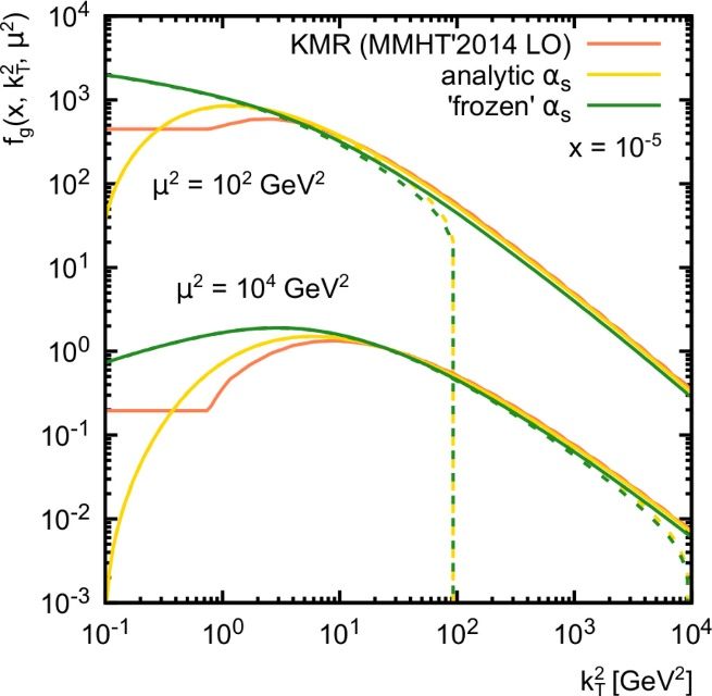
involved in the KMR prescription (namely, angular and strong ordering conditions) and
discuss the relations between the differential and integral formulation of the KMR proce-
dure pointed out recently in [44]. Finally, we present some phenomenological applications
of obtained TMD parton densities to hard LHC processes, sensitive to the quark and gluon
content of the proton. To be precise, using the kT -factorization QCD approach, we consider
                                                     √
the inclusive production of b-jets and bb̄-dijets at s = 7 TeV, inclusive production of the
                                                 √
Higgs bosons (in the diphoton decay mode) at s = 13 TeV and charm and beauty contri-
butions to the deep inelastic proton structure function F2 (x, Q2 ) at different values of Q2 .
    The outline of our paper is following. In section 2 we briefly describe our theoretical

                                                                                                  JHEP02(2020)028
input. The calculations are explained in detail in section 3, where we also present the
modifications of PDFs and TMDs at low Q2 -values and outside of the standard small
x range. Section 4 present numerical results and discussions. Section 5 contains our
conclusions.

2       Theoretical framework

Since the KMR approach is based on the standard PDFs, here we present a review of small
x behaviour of parton densities. Moreover, we introduce the basic formulas of the KMR
approach itself.

2.1       PDFs and proton structure function F2 (x, Q2 )

The fairly reasonable agreement between HERA data [45–49] and the results of NLO per-
turbative QCD evaluations is observed for Q2 ≥ 2 GeV2 (see reviews [50, 51] and references
therein). Therefore, it can be concluded that pQCD is capable of describing the evolution
of proton structure function F2 (x, Q2 ) and its derivatives down to very low Q2 values.
     It was pointed out [52] that the HERA small-x data can be well interpreted in terms
of the so-called doubled asymptotic scaling (DAS) phenomenon related to the asymptotic
behaviour of the DGLAP evolution discovered many years ago [43]. The study [52] was
extended [40–42] to include the finite parts of anomalous dimensions (ADs) of Wilson
operators and Wilson coefficients.1 This led to predictions [39–41] of the small-x asymptotic
form of PDFs in the framework of the DGLAP dynamics, which were obtained starting at
some Q20 with the flat function
                                              fa (x, Q20 ) = Aa ,                         (2.1)

where fa are PDFs multiplied by x, a = q or g and Aa are unknown parameters to
be determined from the data. We refer to the approach of [40–42] as generalized DAS
approximation. In this approach the flat initial conditions (2.1) determine the basic role
of the AD singular parts as in the standard DAS case, whereas the contributions coming
from AD finite parts and Wilson coefficients can be considered as corrections which are,
however, important for achieving better agreement with experimental data.
    1
        In the standard DAS approximation [43] only the AD singular parts were used.

                                                    –3–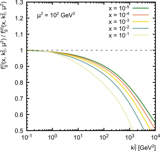
Hereafter we consider for simplicity only the LO approximation, where the structure
function (fi (x, Q2 ) incorporates an x factor as it was already discussed after eq. (2.1))
                                                   f
                                                   X
                                  F2 (x, Q2 ) =           e2i fi (x, Q2 )                    (2.2)
                                                    i=1

can be represented as a sum of the singlet (SI) and nonsinglet (NS) parts:

                             F2 (x, Q2 ) = F2SI (x, Q2 ) + F2NS (x, Q2 )                     (2.3)

Here ei are quark charges and f is a number of active (massless) quark flavors.

                                                                                                      JHEP02(2020)028
                                                              f
    The part F2SI (x, Q2 ) can be expressed as (hereafter e =   e2i /f is an average charge
                                                              P
                                                                            i=1
squared)
                                      F2SI (x, Q2 ) = e fSI (x, Q2 ),                        (2.4)
through the PDF singlet combination
                                      f
                                      X
                     fSI (x, Q2 ) =         fi (x, Q2 ) = fS (x, Q2 ) + fV (x, Q2 )          (2.5)
                                      i=1

which, in turn, is equal to the sea fS (x, Q2 ) and valence fV (x, Q2 ) = uv (x, Q2 ) + dv (x, Q2 )
quark components. The part F2NS (x, Q2 ) is proportional to the PDF nonsinlet conbination
fNS (x, Q2 ) = uv (x, Q2 ) − dv (x, Q2 ).
     Compared to the sea quark part fS (x, Q2 ), all the rest are strongly (powerlike) sup-
pressed at small x values. Therefore, at low x the DIS structure function F2 (x, Q2 ) can be
expressed through the sea part of quark densities fS (x, Q2 ) ≡ fq (x, Q2 ) as

                                      F2 (x, Q2 ) = e fq (x, Q2 ) .                          (2.6)

    The small-x asymptotic expressions for sea quark and gluon densities fa (x, µ2 ) can be
written as follows (both the LO and NLO results and their derivation can be found [39, 40]):

                        fa (x, µ2 ) = fa+ (x, µ2 ) + fa− (x, µ2 ),

                       fg (x, µ ) = Ag + C Aq I 0 (σ) e−d+ s + O(ρ),
                         +      2


                                      ϕ
                       fq+ (x, µ2 ) =      Ag + C Aq I˜1 (σ) e−d+ s + O(ρ),
                                      3
                       fg− (x, µ2 ) = −C Aq e−d− s + O(x),
                       fq− (x, µ2 ) = Aq e−d− s + O(x),                                      (2.7)

where C = CF /CA and ϕ = f /CA and CA = Nc , CF = (Nc2 − 1)/(2Nc ) for the color
SU(Nc ) group. In QCD case, Nc = 3 and, thus, CA = 3, CF = 4/3, C = 4/9 and ϕ = f /3.
     Here I ν (σ) and I˜ν (σ) (ν = 0, 1) are the combinations of the modified Bessel functions
(at s ≥ 0, i.e. µ2 ≥ Q20 ) and the usual Bessel functions (at s < 0, i.e. µ2 < Q20 ):
                       (                                       (
                         ρ ν I (σ),
                              ν          if s ≥ 0;               ρ−ν Iν (σ), if s ≥ 0;
             I˜ν (σ) =                             , I ν (σ) =                           (2.8)
                         (−ρ̃)ν Jν (σ̃), if s < 0.               ρ̃−ν Jν (σ̃), if s < 0.

                                                  –4–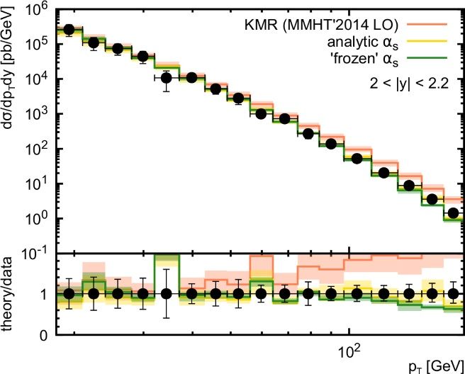
where I 0 (σ) = I˜0 (σ) and
s
as (Q20 ) αs (µ2 )
1 1
s = ln , a s (µ 2
) ≡ = , σ=2 dˆ+ s ln ,
2
as (µ ) 4π β0 ln(µ2 /Λ2LO ) x
s
σ 1 σ̃
ρ= , σ̃ = 2 − dˆ+ s ln , ρ̃ = (2.9)
2 ln(1/x) x 2 ln(1/x)
and
4CA 12 4f (1 − C) 20f 4Cf 16f
dˆ+ = − =− , d+ = 1 + =1+ , d− = = (2.10)
β0 β0 3β0 27β0 3β0 27β0
JHEP02(2020)028
are the singular and regular parts of the anomalous dimensions and β0 = 11 − (2/3)f is
the first coefficient of the QCD β-function in the MS-scheme.
The results for the parameters Aa and Q20 can be found in [39, 53–55]; they were
obtained2 for αs (MZ ) = 0.1168.
It is convenient to show the following expressions:
CA 4Cf 4CA ϕ
β0 dˆ+ = −4CA , β0 d+ = 11 − 2ϕ(1 − 2C) , β0 d− = = . (2.11)
3 3 3
2.2 Kimber-Martin-Ryskin approach
The expressions (2.3)–(2.6) can be used as an input for the KMR procedure [32, 33],
giving us the possibility to calculate the TMD parton density functions in a proton. Let
(d)
k⊥ ≡ k, then the TMD parton distributions in the differential fa (x, k 2 , µ2 ) and integral
(i)
fa (x, k 2 , µ2 ) formulation of the KMR approach can be written as
∂ h i
fa(d) (x, k 2 , µ2 ) = T a (µ 2 2
, k )D a (x, k 2
) , (2.12)
∂ ln k 2
x0
X Z dz x
(i) 2 2 2 2
fa (x, k , µ ) = Ta (µ , k ) Paa0 (z, k 2 ) Da , k 2 , x0 = 1 − ∆ , (2.13)
0
z z
a x
where Da (x, µ2 ) are the conventional PDFs, fa (x, µ2 ) = xDa (x, µ2 ), which obey the
DGLAP equations (see (2.1) in [44]):
Zx0 Zx0
∂Da (x, µ2 ) X dz x X
= Paa0 (z, µ2 ) Da , µ2 − Da (x, µ2 ) dz zPa0 a (z, µ2 ) (2.14)
∂ ln µ2 0
z z 0
a x a 0
with the splitting functions
(LO)
Paa0 (z, µ2 ) = 2as (µ2 ) Paa0 (z, µ2 ) + . . . . (2.15)
The Sudakov form factor Ta (µ2 , k 2 ) has the following form (see (2.4) in [44]):
2
Zµ dp2 X Zx0
2 2 2
Ta (µ , k ) = exp − 2
dz zP a 0 a (z, k ) . (2.16)
2 p
a0
k 0
2
In the future, by using (2.6) and (2.7) and results of [56, 57] we plan to perform the combined fits to
the H1 and ZEUS experimental data [49] and [58] for the DIS structure function F2 (x, Q2 ) and its charm
part F2c (x, Q2 ), respectively.
–5–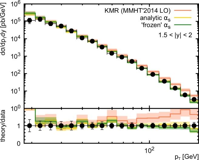
3     Calculations

The DGLAP splitting functions at LO can be presented as (see, for example, (2.56)–(2.60)
in [59])

                         1 + z2

                                    3                        h             i
         Pqq (z) = CF            + δ(1 − z) , Pqg (z) = f z 2 + (1 − z)2 ,
                        (1 − z)+ 2
                        1 + (1 − z)2

         Pgq (z) = CF                  ,                                           (3.1)
                              z

                             z        1−z               11 − 2ϕ
         Pgg (z) = 2CA            +        + z(1 − z) +         δ(1 − z) .

                                                                                                           JHEP02(2020)028
                         (1 − z)+        z                 12

Since the upper limit of integrals in the r.h.s. of (2.10) and (2.16) is restricted by x0 ≡ 1−∆,
the δ-functions in (2.13) give no contributions. Moreover, the “+” prescription is not
needed: (1 − z)−1
               + → (1 − z) .
                              −1

3.1     Sudakov form factors Ta (µ2 , k2 )
Evaluating (2.16), we have
                                                      h            i
                                  Ta (µ2 , k 2 ) = exp −da Ra (∆)s1 ,                              (3.2)

where
                     as (k 2 )

                                          4Ca                                   CA
            s1 = ln              , d a =       , C q =  C F , C g = C A , β 0 =      11 − 2ϕ   ,
                     as (µ2 )              β0                                    3
                               3x2

                     1                       1       3
        Rq (∆) = ln        − 0 = ln              − (1 − ∆)2 ,
                     ∆          4           ∆        4

                     1                ϕ 2 1−ϕ 3

        Rg (∆) = ln        − 1−           x0 +         x (4 − 3x0 ) =
                     ∆                4           12 0

                     1                ϕ               1−ϕ
               = ln        − 1−           (1 − ∆)2 +          (1 − ∆)3 (1 + 3∆) .                  (3.3)
                     ∆                4                  12

3.2     TMDs from differential formulation of KMR approach
Now we can use (2.12) to find the results for TMD parton densities without derivatives.
Derivation of Ta (µ2 , k 2 ) is as follows

                                 ∂Ta (µ2 , k 2 )
                                                 = da β0 as (k 2 ) Ra (∆),                         (3.4)
                                   ∂ ln k 2
and derivations of conventional PDFs are as follows
                                         "         !                          #
             ∂fa (x, k 2 )            2    dˆ+       +      2        −      2
                           = −β0 as (k )       + d+ fa (x, k ) + d− fa (x, k ) ,                   (3.5)
              ∂ ln k 2                      ρa

where
                                     1    I 1 (σ)   1   I 0 (σ)
                                        =         ,   =         .                                  (3.6)
                                     ρg   I 0 (σ) ρq    I˜1 (σ)

                                                  –6–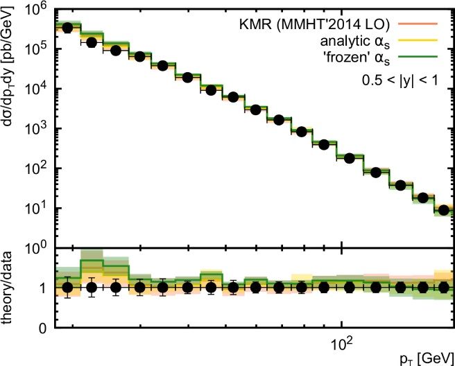
So, the result for the TMD parton densities reads
fa(d) (x, k 2 , µ2 )
" ! #!
ˆ+
d
= β0 as (k 2 )Ta (µ2 , k 2 ) da Ra (∆) fa (x, k 2 )− +d+ fa+ (x, k 2 )+d− fa− (k 2 )
ρa (3.7)
" ! #!
1 dˆ+
= 4Ca as (k 2 )Ta (µ2 , k 2 ) Ra (∆) fa (x, k 2 )− +d+ fa+ (x, k 2 )+d− fa− (k 2 ) .
da ρa
The expressions for conventional PDFs and Sudakov form factors are given in the sections 2
JHEP02(2020)028
and 3.1, respectively. Since the value of dˆ+ is negative and the factor dˆ+ /ρa is large at low
(d)
x, the TMDs fa (x, k 2 , µ2 ) are positive at small x. With increasing x, the results for the
latter can be negative.
3.3 TMDs from integral formulation of KMR approach
Now we can use (2.13) to find the results for TMDs without derivatives. After some algebra
we have
fa(i) (x, k 2 , µ2 ) = 4Ca as (k 2 )Ta (µ2 , k 2 )×
x 2 x 2 x 2
× Sa (∆) fa , k + Sa+ fa+ , k + Sa− fa− ,k =
x0 x0 x0 (3.8)
2 2 2 x 2 + + x 2
= 4Ca as (k )Ta (µ , k ) S a (∆) fa , k + S a fa ,k ,
x0 x0
where
+
S a (∆) = Sa (∆) + Sa− , S a = Sa+ − Sa− . (3.9)
Using the relations from (2.11), we can obtain:
1 x0 1 1−∆
Sq (∆) = ln − (2 + x0 ) = ln − (3 − ∆),
∆ 4 ∆ 4
x2 x3
1 1 1−∆
Sg (∆) = ln − x0 + 0 − 0 = ln − (13 − 5∆ + 4∆2 ),
∆ 4 3 ∆ 12
2x20
− x0 ϕ (1 − ∆)ϕ
Sq (∆) = − 1 − x0 + =− (2 − ∆ + 2∆2 ), Dg− (∆) = 0,
2 3 6
1 x2 Cϕ
Sg+ = − x0 + 0 + ,
ρg 4 3
" #
2x20 x0 2x20
+ 3x0 1
Sq = 1 − x0 + − 1− + , (3.10)
2C ρs 3 2 9
where
σ x → x
x0 , if s ≥ 0;
1 1 x
σ= , = x→ . (3.11)
σ̃ x → x ρa ρa x0
x0 , if s < 0.
–7–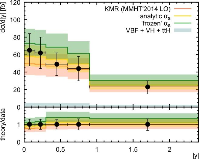
3.4 Cut-off parameter ∆
For the phenomenological applications, the cut-off parameter ∆ usually has one of two
basic forms:
k k
∆1 = , ∆2 = , (3.12)
µ k+µ
that reflects the two cases: ∆1 is in the strong ordering, ∆2 is in the angular ordering
(see [44]). In all above cases, except the results for Ta (µ2 , k 2 ), we can simply replace the
parameter ∆ by ∆1 and/or ∆2 . For the Sudakov form factors, we note that the parameters
JHEP02(2020)028
∆i (with i = 1, 2) contribute to the integrand in (2.16) and, thus, their momentum depen-
dence changes the results in (3.2). To perform the correct evaluation of the integral (2.16),
we should recalculate the p2 integration in (2.16). So, we have
2
Zµ
dp2
Ta(i) (µ2 , k 2 ) = exp −4Ca as (p2 )Ra (∆i ) . (3.13)
p2
k2
(i)
The analytic evaluation of Ta (µ2 , k 2 ) is a very cumbersome procedure, which will be
accomplished in the future. With the purpose of simplifying our analysis, below we use the
(i)
numerical results for Ta (µ2 , k 2 ).
3.5 Comparison of fa(i) (x, k2 , µ2 ) and fa(d) (x, k2 , µ2 )
To perform the comparison between the two obtained expressions, it is convenient to
rewrite (3.7) as
fa(d) (x, k 2 , µ2 ) = 4Ca as (k 2 )Ta (µ2 , k 2 )×
− −
× Ra (∆) fa (x, k 2 ) + t+ + 2 2
a fa (x, k ) + ta fa (x, k ) = (3.14)
+
= 4Ca as (k 2 )Ta (µ2 , k 2 ) Ra (∆) fa (x, k 2 ) + ta fa+ (x, k 2 ) ,
where
!
1 dˆ+ d− +
t+
a =− + d+ , t−
a =− , Ra (∆) = Ra (∆) + t− + −
a , ta = ta − t a . (3.15)
da ρa da
Using the relations from (2.11), we can obtain:
1 1 Cϕ
t+
g = − 11 + 2ϕ(1 − 2C) , t−
g =− ,
ρg 12 3
(3.16)
+ 1 1 1 ±
tg = − 11 + 2ϕ(1 − 4C) , t±
q = t (ρg → ρq ).
ρg 12 C g
–8–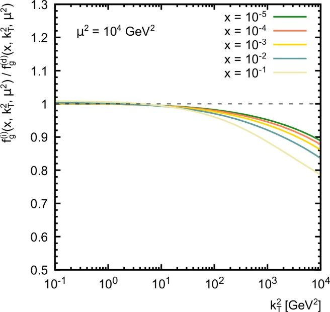
JHEP02(2020)028
Figure 1. The ratio of the TMD gluon densities in a proton obtained using integral and differential
formulation of the KMR approach as a function of the gluon transverse momentum kT2 at different
values of longitudinal momentum fraction x and hard scale µ2 . The angular ordering condition was
applied.

                                                 (i)                 (d)
It is convenient to compare the results for fa (x, k 2 , µ2 ) and fa (x, k 2 , µ2 ), i.e. the values
               +                   +
of S a (∆), S a (∆) and Ra (∆), ta (∆) at ∆ → 0, when k 2  µ2 :

                       1      3 ϕ                                   1      11 ϕ(1 − 2C)
      Rq (∆) = ln          − − ,                    Rg (∆) = ln         −      +               ,
                      ∆       4   3                                 ∆      12           6

                       1      3 ϕ                                   1      13
      S q (∆) = ln         − − ,                   Dg (∆) = ln          − ,
                      ∆       4   3                                 ∆      12

             +    1 1        11 ϕ(1 − 4C)                +     1     11 ϕ(1 − 4C)
           tq =           −     −             ,         tg =       −    −                ,
                  C ρq       12        6                       ρg    12         6

             +    1 1        13 Cϕ                       +     1     3 Cϕ
           Sq =           −     +       ,               tg =       − +        ,               (3.17)
                  C ρq       12    3                           ρg    4     3
or
                                                                      1
      Rq (∆) = S q (∆),                         Rg (∆) = Dg (∆) +        1 + ϕ(1 − 2C) ,
                                                                      6
             +      +    1
                                                     +      +     1
            tq = S q +      1 − ϕ(1 − 2C) ,         tg = S g −       1 + ϕ(1 − 2C) .          (3.18)
                         6                                        6
So, the difference is regular at ∆ → 0 and it does not give large contributions. This is
                                                                                 (i)
clearly illustrated in figure 1, where we show the ratio of gluon densities fa (x, k 2 , µ2 ) and
  (d)
fa (x, k 2 , µ2 ) calculated with angular ordering condition applied as a function of kT2 ≡ k 2
at several values of x and µ2 . As one can see, with increasing k 2 the difference between
these two approaches becomes more pronounced.

3.6   Infrared modification of the strong coupling
The equations (2.7) at s < 0 were used in [41], where the higher-twist corrections through
twist six were added to find good agreement with the experimental data for the deep inelatic

                                               –9–
proton structure function F2 (x, Q2 ) for Q2 ≥ 0.5 GeV2 . However, such application is not
so useful here because the case with s < 0 may lead to the negative TMDs and, hence, to
the negative cross sections of the physical processes.
To overcome these problems, which emerge at small k 2 values, we investigate an alter-
native possibility following to [39]; namely, the modification of the strong-coupling constant
in the infrared region. Specifically, we consider two modifications, which effectively increase
the argument of the strong coupling constant at small µ2 values, in accordance with [60–63].
In the first case, which is more phenomenological, we introduce a freezing of the strong-
coupling constant by changing its argument as µ2 → µ2 + Mρ2 , where Mρ is the ρ meson
mass [64]. Thus, in the formulae of section 3 we introduce the following replacement
JHEP02(2020)028
αs (µ2 ) → αfr (µ2 ) = αs (µ2 + Mρ2 ) . (3.19)
The second possibility is based on the idea by Shirkov and Solovtsov [65, 66] (see also the
recent reviews [67–69] and the references therein) regarding the analyticity of the strong
coupling that leads to an additional power dependence. In this case, the QCD coupling
αs (µ2 ) appearing in the formulae of the previous sections is to be replaced as
1 Λ2LO
αs (µ2 ) → αan (µ2 ) = αs (µ2 ) − . (3.20)
β0 µ2 − Λ2LO
Such replacements have been done [39], where we took the normalizations magnitudes Ag
and Aq . As we can see from [39, 53–55], the fits based on the frozen and analytic strong-
coupling constants are very similar and describe the F2 (x, Q2 ) data in the small-Q2 range
significantly better than the canonical fit.
3.7 Beyond small x
In the phenomenological applications (see section 4) the calculated TMD parton densities
will be used to predict the cross sections of several high-energy processes. According to
kT -factorization approach [4–7], the theoretical predictions for the cross sections can be
obtained by convolution of these TMD parton densities and the corresponding off-shell
production amplitudes. So, we need the TMD quark and gluon distributions in rather
broad range of the x variable, i.e. beyond the standart low x range (x ≤ 0.05).
Our TMD parton densities are exactly expressed through the conventional PDFs
fa (x, µ2 ) as it was shown in the equations (3.14) and (3.8). Then, the densities fa (x, µ2 )
listed in section 2.1 should be extended in the following form [70–73] (see, for example, the
recent paper [74], where similar extension has been done in the case of EMC effect from
the study of shadowing [75] at low x to antishadowing effect at x ∼ 0.1–0.2):
4Ca s
fa (x, µ2 ) → fa (x, µ2 ) (1 − x)βa (s) , βa (s) = βa (0) + . (3.21)
β0
Note that such form was successfully used in the conventional PDF parametrizations
(see [72, 73, 76]). The value of βa (0) can be estimated from the quark counting rules [77–79]:
βv (0) ∼ 3, βg (0) ∼ βv (0) + 1 ∼ 4, βq (0) ∼ βv (0) + 2 ∼ 5 , (3.22)
– 10 –where the symbol v marks the valence part of quark density. Usually the βv (0), βg (0),
βq (0) are determined from fits of experimental data (see, for example, [80–86]) and the
results for these values may be quite different, because various groups producing PDF sets
use different sets of experimental data or take some privilege for their parts. Moreover, the
difference can be attributed to various choices of the initial condition µ20 of the µ2 -evolution
but it should be not so strong because the µ2 -dependence is double-logarithmic.
It is convenient to assume that similar relations take place just beyond the standard
low x range (x ≤ 0.05). Thus, the TMD parton densities can be modified in the form,
similar to (3.17), that leads to
JHEP02(2020)028
fa(d) (x, k 2 , µ2 ) → fa(d) (x, k 2 , µ2 ) (1 − x)βa (s) , (3.23)
x βa (s)
(i) 2 2 (i) 2 2
fa (x, k , µ ) → fa (x, k , µ ) 1 − . (3.24)
x0
In our analysis, the numerical values of βg (0) have been extracted from the fit to the
inclusive b-jet production data taken by the CMS [87] and ATLAS [88] Collaborations in pp
√
collisions at s = 7 TeV (see section 4.1 below). We find that best description of the leading
b-jet transverse momentum distributions in a whole kinematical region is achieved with
βg (0) = 5.77 and βg (0) = 3.84 for “frozen” and analytic strong coupling constant (3.19)
and (3.20), respectively. We see that the obtained results are close to ones in (3.22).
The TMD gluon densities in a proton obtained with appropriate treatment of the
strong coupling and βg (0) are shown in figure 2 as a function of transverse momentum kT2
for different values of proton longitudinal momentum fraction x and hard scale µ2 . We have
used the integral formulation of KMR procedure as given by (3.20) for illustration. The
solid green and yellow curves correspond to the results obtained with “frozen” and ana-
lytic coupling constant with angular ordering condition, while corresponding dashed curves
represent the results obtained with strong ordering condition. As one can see, the strong
ordering condition leads to a steep drop of the gluon densities beyond the scale µ2 . It con-
trasts with angular ordering, where the gluon transverse momentum is allowed to be larger
than µ2 (see [44]). We also show here the TMD gluon distributions calculated numerically
in the traditional KMR scenario, where the conventional parton densities from standard
MMHT’2014 (LO) set [89] were used as an input (red curves on figure 2). The results of our
analytical calculations are nicely agree with the latter for kT2 ≥ 10 GeV in wide x region (up
to x ≤ 0.05), that demonstrates the applicability of the generalized DAS approximation.
At kT2 < µ20 ∼ 1 GeV2 the numerically calculated KMR gluon density is modelled to be a
flat according to the prescription [32, 33] under strong normalization condition
2
Zµ
fa (x, k 2 , µ2 )dk 2 = fa (x, µ2 ), (3.25)
0
which is often used in the KMR scheme. Such determination, of course, leads to a low kT2
plateau, clearly seen in figure 1. In contrast, our formalism with appropriate modifications
of strong coupling as described above results in continuous TMD quark and gluon density
functions, well defined in a whole kT2 region. Below we will consider the phenomenological
consequences of our approach.
– 11 –JHEP02(2020)028
Figure 2. The TMD gluon densities in a proton calculated as a function of the gluon transverse
momentum kT2 at different values of longitudinal momentum fraction x and hard scale µ2 . The
integral formulation of the KMR approach is used. The solid green and yellow curves correspond
to the results obtained with “frozen” and analytic QCD coupling constant with angular ordering
condition, while corresponding dashed curves represent the results obtained with strong ordering
condition. The red curves correspond to the TMD gluon distributions calculated numerically in
the traditional KMR scenario, where the conventional parton densities from standard MMHT’2014
(LO) set are used as an input.
– 12 –4 Phenomenological applications
We are now in a position to apply the obtained TMD parton densities in a proton to
several hard QCD processes studied at hadron colliders. In the present paper we consider
the inclusive production of b-jets and Higgs bosons at the LHC conditions and charm and
beauty contributions to the deep inelastic proton structure function F2 (x, Q2 ) measured
in ep collisions at HERA. These processes have been already investigated within the kT -
factorization approach and found to be strongly sensitive to the gluon content of the proton.
To calculate the total and differential cross sections of b-jets, Higgs boson production
and proton structure functions F2c (x, Q2 ) and F2b (x, Q2 ) we strictly follow our previous
JHEP02(2020)028
considerations [19, 20, 23, 24, 90, 91]. Everywhere below we have used one-loop formula
for the strong coupling constant with nf = 4 active quark flavors and ΛQCD = 143 MeV
(that corresponds to αs (m2Z ) = 0.1168) for analytically calculated TMD quark and gluon
densities as described above and apply nf = 5 with αs (m2Z ) = 0.13 for KMR partons
evaluated numerically. The latter choice is dictated by the parameter setup employed in
the MMHT’2014 (LO) PDFs [89], used here as an input for KMR procedure.
4.1 Inclusive b-jet production at the LHC
Following [23, 24], our consideration is based on the leading off-shell (depending on the
transverse momenta of incoming particles) gluon fusion subprocess g ∗ (k1 )+g ∗ (k2 ) → b(p1 )+
b̄(p2 ), where the four-momenta of all particles are indicated in parentheses. According to
the kT -factorization prescription [4–7], the corresponding cross section can be written as
Z Z
σ = dx1 dx2 dk21T dk22T fg (x1 , k21T , µ2 )fg (x2 , k22T , µ2 )×
(4.1)
∗ 2 2 2
× dσ (x1 , x2 , k1T , k2T , µ ),
where σ ∗ (x1 , x2 , k21T , k22T , µ2 ) is the off-shell partonic cross section and k21T and k22T are
the non-zero two-dimensional transverse momenta of incoming partons. The detailed de-
scription of the calculation steps (including the evaluation of the off-shell amplitudes) can
be found in [23, 24]. Here we only specify the essential numerical parameters. So, follow-
ing [92], we set the b-quark mass mb = 4.78 GeV and, as it often done in pQCD calculations,
choose the default renormalization and factorization scales µR and µF to be equal to lead-
ing b-jet transverse momentum. The calculations were performed using newly developed
Monte-Carlo event generator pegasus [93, 94].
The CMS Collaboration has measured the double differential cross section dσ/dpT dy
√
of inclusive b-jet production at s = 7 TeV in five b-jet rapidity regions, namely, |y| < 0.5,
0.5 < |y| < 1, 1 < |y| < 1.5, 1.5 < |y| < 2 and 2 < |y| < 2.2 as a function of the leading b-jet
transverse momentum [87]. In the ATLAS analysis [88], the inclusive b-jet cross section has
been measured as a function of transverse momentum pT in the range 20 < pT < 400 GeV
and rapidity in the range |y| < 2.1. In addition, the bb̄-dijet cross section has been measured
as a function of the dijet invariant mass M in the range 110 < M < 760 GeV, azimuthal
angle difference ∆φ between the two b-jets and angular variable χ = exp |y1 − y2 | for jets
with pT > 40 GeV in two dijet mass regions.
– 13 –The results of our calculations are shown in figures 3–5 in comparison with the CMS
and ATLAS data [87, 88]. The solid green and yellow histograms were obtained with
the TMD gluon density as given by (3.4)–(3.7) with “frozen” and analytic QCD coupling
by fixing both the renormalization and factorization scales at their default values. The
red histograms represent the results obtained with the numerically calculated KMR gluon
distributions. The shaded bands correspond to scale uncertainties of these predictions. As
usual, the latter have been estimated by varying the scales µR and µF by a factor of 2
around their default values. We have obtained a good description of the b-jet transverse
momentum distributions in each of the rapidity subdivisions, both in normalization and
the shape. Our predictions are only tend to slightly underestimate the measured cross
JHEP02(2020)028
sections at very high transverse momenta pT ∼ 200–400 GeV, but they agree with the
data within the theoretical and experimental uncertainties. The results obtained with
numerically calculated KMR gluon density agree with data and analytical TMD gluons at
low and moderate transverse momenta, but overestimate both the CMS and ATLAS data
at pT > 100 GeV, especially at forward rapidities. We note that here the essentially large x
region is probed, so the better description of the data achieved with analytical TMD gluon
distributions demonstrates that their large-x extension, as described above in section 3.7,
is rather reasonable.
All the considered TMD gluons show good agreement with the bb̄-dijet cross sections
measured by the ATLAS Collaboration. In particular, the good description of the ∆φ dis-
tribution is remarkable, since the latter is known to be a strongly sensitive to the kT2 shape
of the TMD gluon density (see [23, 24] and references therein). As it was expected, the χ
distribution flattens for large invariant masses M . Note that here an additional acceptance
requirement, that restricts the boost of the dijet system to |yboost | = |y1 + y2 |/2 < 1.1, has
been applied for χ measurements. This requirement significantly reduces [88] the sensitiv-
ity to gluon density function at small x and all theoretical predictions for χ distributions
are practically coincide. Thus, we conclude that our analytical TMD parton densities given
by (3.4)–(3.7) does not contradict available LHC data on b-jet production.
4.2 Inclusive Higgs boson production at the LHC
Our consideration is mainly based on the off-shell amplitude of the gluon-gluon fusion sub-
process g ∗ (k1 ) + g ∗ (k2 ) → H(p) calculated using the effective Lagrangian [95, 96] for the
Higgs coupling to gluons and extended recently to the subsequent H → γγ, H → ZZ ∗ → 4l
(where l = e or µ) and H → W + W − → e± µ∓ ν ν̄ decays. The details of the calculations
are explained in [19, 20] and here we strictly follow our previous consideration. Every-
where below, we set the Higgs boson mass mH = 125.1 GeV and its full decay width
ΓH = 4.3 MeV. The default values of the renormalization and factorization scales are
chosen to be equal to Higgs mass. The cross sections were produced with Monte-Carlo
generator pegasus [93, 94].
The latest measurements of the inclusive Higgs boson production (in the diphoton de-
cay mode) were performed by the CMS [97] and ATLAS [98] Collaborations at the LHC
√
energy s = 13 TeV. In the CMS analysis, two isolated final state photons originating
from the Higgs boson decays are required to have pseudorapidities |η γ | < 2.5, excluding
– 14 –JHEP02(2020)028
√
Figure 3. The transverse momentum distributions of inclusive b-jet production at s = 7 TeV as
a function of the leading jet transverse momentum in different rapidity regions. The kinematical
cuts are described in the text. Notation of histograms is the same as in figure 1. The experimental
data are from CMS [87].
– 15 –JHEP02(2020)028
√
Figure 4. The transverse momentum distributions of inclusive b-jet production at s = 7 TeV as
a function of the leading jet transverse momentum in different rapidity regions. The kinematical
cuts are described in the text. Notation of histograms is the same as in figure 1. The experimental
data are from ATLAS [88].
– 16 –JHEP02(2020)028
Figure 5. The dijet invariant mass M , azimuthal angle difference ∆φ and χ distributions of bb̄-dijet
√
production at s = 7 TeV. The kinematical cuts are described in the text. The experimental data
are from ATLAS [88].
the region 1.4442 < |η γ | < 1.566. Additionally, photons with largest and next-to-largest
transverse momentum pγT (so-called leading and subleading photons) must satisfy the con-
ditions of pγT /M γγ > 1/3 and pγT /M γγ > 1/4 respectively, where M γγ is the diphoton pair
mass, M γγ > 90 GeV. In the ATLAS measurement [98] both of these decay photons must
have pseudorapidities |η γ | < 2.37 (excluding 1.37 < |η γ | < 1.52) with the leading (sublead-
ing) photon satisfying pγT /M γγ > 0.35 and pγT /M γγ > 0.25, while invariant mass M γγ is
required to be 105 < M γγ < 160 GeV. We have implemented experimental setup in our nu-
merical program. The Higgs transverse momentum pT , absolute value of the rapidity y and
cosine of photon helicity angle cos θ∗ (in the Collins-Soper frame) were measured [97, 98].
Both pT and y probe the production mechanism and parton distribution functions in a
proton, while cos θ∗ is related to spin-CP nature of the decaying Higgs boson.
The results of our calculations are shown in figures 6 and 7 in comparison with latest
LHC data. One can see that our predictions with both analytic and “frozen” treatment of
QCD coupling reasonably agree with the data for all considered kinematical observables,
although some tendency to slightly overestimate the LHC data in the low pT region is
observed. This tendency results in a some ovestimation of the rapidity and photon helicity
– 17 –JHEP02(2020)028
Figure 6. The differential cross sections of inclusive Higgs boson production (in the diphoton decay
√
mode) at s = 13 TeV as functions of diphoton pair transverse momentum pγγ T , rapidity y
γγ
and
∗
photon helicity angle cos θ (in the Collins-Soper frame). The experimental data are from CMS [97].
angle distributions, but the predictions are still agree with the data within the experimental
and theoretical uncertainties, calculated as it was described above. The scale dependence
of our predictions, of course, exceeds the uncertainties of conventional higher-order pQCD
calculations (which are about of 10–11%). However, it could be easily understood be-
cause only the tree-level LO hard scaterring amplitudes are involved. The strong drop in
the | cos θ∗ | distribution around | cos θ∗ | ∼ 0.6 is due to the fiducial requirement on the
photon system originating from the scalar Higgs boson decay. The calculations based on
the numerically evaluated KMR gluon density agree well with the data at low pT and
tend to overshoot them at high transverse momenta. Note that we added to our results
contributions from weak boson fusion (W + W − → H and ZZ → H), associated HZ or
HW ± production and associated tt̄H production (grey shaded bands in figures 6 and 7).
These contributions are essential at high pT and have been calculated in the conventional
pQCD approach with the NLO accuracy. We take them from [97, 98]. Once again, we
can conclude that the analytical expressions for TMD parton densities (3.4)–(3.7) does not
contradict available LHC data in the probed kinematical region, where µ2 ∼ m2H .
– 18 –JHEP02(2020)028
Figure 7. The differential cross sections of inclusive Higgs boson production (in the diphoton
√
decay mode) at s = 13 TeV as functions of diphoton pair transverse momentum pγγ T , rapidity
γγ ∗
y and photon helicity angle cos θ (in the Collins-Soper frame). The experimental data are from
ATLAS [98].
4.3 Proton structure functions F2c (x, Q2 ) and F2b (x, Q2 )
The important information on the quark and gluon structure of proton can be also extracted
from the data on deep inelastic ep scattering. Its differential cross section can be presented
in the simple form:
d2 σ 2πα2 y2 y2
2 2
= 1 − y + F 2 (x, Q ) − F L (x, Q ) , (4.2)
dxdy xQ4 2 2
where F2 (x, Q2 ) and FL (x, Q2 ) are the proton transverse and longitudinal structure func-
tions, x and y are the usual Bjorken scaling variables. The charm and beauty contributions
to F2 (x, Q2 ) are described through perturbative production of charm or beauty quarks and,
therefore, directly related with the gluon content of the proton. Our evaluation below is
based on the formulas [90, 91] and here we again strictly follow our previous consideration
in all aspects. We only note that the charm and beauty masses are set to be equal to
mc = 1.65 GeV and mb = 4.78 GeV [92].
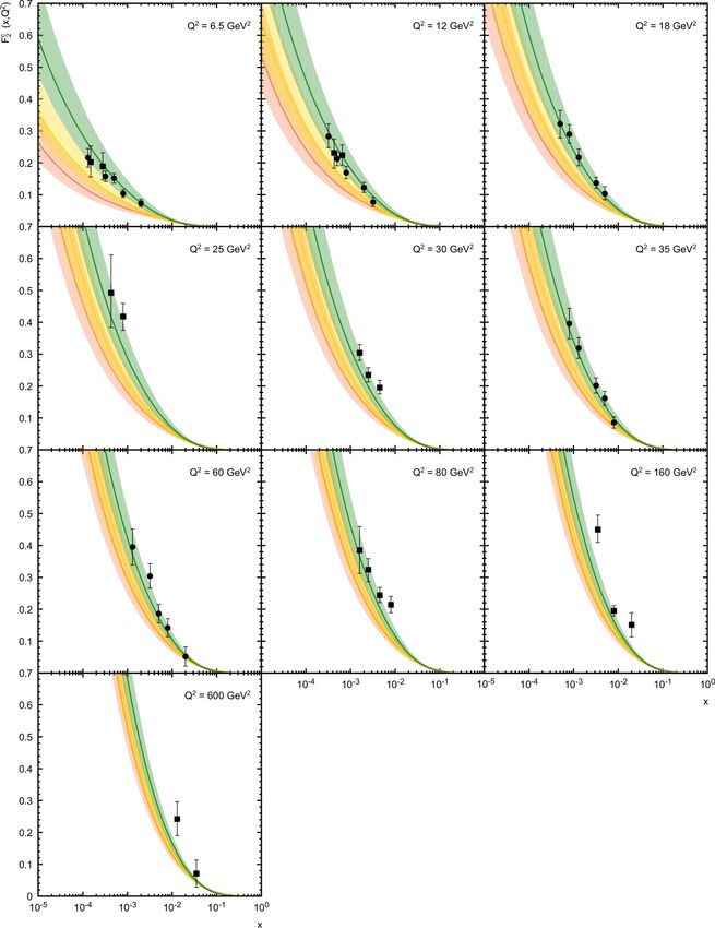
Our results are shown in figures 8 and 9 in comparison with the latest ZEUS [99] and
H1 [100, 101] data. We find that the predictions obtained with “frozen” strong coupling are
– 19 –in good agreement with the latest HERA data for both structure functions F2c (x, Q2 ) and
F2b (x, Q2 ) in a wide region of x and Q2 , both in normalization and shape. These predictions
slightly overshoot the ones obtained with analytic treatment of the QCD coupling constant.
The difference between these two approaches becomes more clearly pronounced at small x
and low Q2 values, Q2 ≤ 10 GeV2 . The predictions based on the analytic QCD coupling
still agree with the data on F2b (x, Q2 ) within the theoretical and experimental uncertainties,
but clearly underestimate the data on F2c (x, Q2 ), especially at low Q2 . However, we note
that some reasonable variation in charmed quark mass mc = 1.65 ± 0.2 GeV can almost
eliminate the visible disagreement (not shown in figures 8 and 9). The traditional KMR
approach underestimates the HERA data on both F2c (x, Q2 ) and F2b (x, Q2 ) at small x and
JHEP02(2020)028
relatively low Q2 ≤ 30–60 GeV2 , where the higher-order QCD corrections are known to be
important. The difference between all the theoretical predictions becomes negligible with
increasing of Q2 . Thus, we can conclude that the proposed analytical calculations of the
TMD parton densities in a proton does not contradict the latest HERA data, although the
best description of the latter (with the default parameter set) is achieved with “frozen”
QCD coupling constant.
5 Conclusions
We presented the analytical calculations of the transverse momentum dependent parton
densities in a proton. These calculations are based on the Bessel-inspired behavior of
parton densities at small Bjorken x, obtained in the case of the flat initial conditions for
DGLAP evolution equations in the double scaling QCD approximation. To construct the
TMD parton distributions we applied the leading-order Kimber-Martin-Ryskin approach,
which is widely used in the phenomenological applications. We implemented the different
treatments of kinematical constraint, reflecting the angular and strong ordering conditions
and discussed the relations between the differential and integral formulation of the KMR
approach. Finally, we demonstrated that the calculated TMD parton distributions does
√
not contradict the LHC data on inclusive b-jet production at s = 7 TeV, inclusive Higg
√
boson production (in diphoton decay mode) at s = 13 TeV and latest HERA data on the
charm and beauty contributions to the deep inelastic proton structure function F2 (x, Q2 )
in a wide region of x and Q2 .
As the next step, we plan to repeat our investigations with taking into account the
precise combined H1 and ZEUS experimental data [49] for the SF F2 (x, Q2 ). Moreover, we
plan to study the longitudinal structure function FL (x, Q2 ) and also to provide predictions
for its heavy quark parts, FLc (x, Q2 ) and FLb (x, Q2 ). The results of these calculations will
be compared with the latest HERA data [102] on the reduced cross sections σred cc̄ and σ bb̄
red
measured very recently by the H1 and ZEUS Collaborations in deep inelastic ep scattering
in a wide Q2 range. Moreover, we plan to extend the present analysis beyond the LO
approximation. We will obtain the results for the NLO TMD parton densities using the
corresponding NLO results [39–41] for the standard PDFs in the generalized DAS approach
and apply the recent results for the NLO matrix elements (see [37, 103–105] and references
and discussions therein) in the subsequent phenomenological analyses.
– 20 –JHEP02(2020)028
Figure 8. The charm contribution to the proton structure function F2 (x, Q2 ) as a function of x
calculated at different Q2 . Notation of curves is the same as in figure 1. The experimental data are
from ZEUS [99] and H1 [100].
– 21 –JHEP02(2020)028
Figure 9. The beauty contribution to the proton structure function F2 (x, Q2 ) as a function of x
calculated at different Q2 . Notation of curves is the same as in figure 1. The experimental data are
from ZEUS [99] and H1 [101].
– 22 –Acknowledgments
We thank H. Jung, S.P. Baranov and M.A. Malyshev for very useful discussions and re-
marks. A.V.K. highly appreciates the warm hospitality at the Institute of Modern Physics
CAS (Lanzhou, China) and thanks the CAS President’s International Fellowship Initiative
(Grant No. 2017VMA0040) for support. A.V.L. is grateful to Institute of Modern Physics
CAS (Lanzhou, China) for support and warm hospitality and DESY Directorate for the
support in the framework of Cooperation Agreement between MSU and DESY on phe-
nomenology of the LHC processes and TMD parton densities. P.Z. is supported in part by
the National Natural Science Foundation of China (Grants No. 11975320).
JHEP02(2020)028
Open Access. This article is distributed under the terms of the Creative Commons
Attribution License (CC-BY 4.0), which permits any use, distribution and reproduction in
any medium, provided the original author(s) and source are credited.
References
[1] R. Angeles-Martinez et al., Transverse Momentum Dependent (TMD) parton distribution
functions: status and prospects, Acta Phys. Polon. B 46 (2015) 2501 [arXiv:1507.05267]
[INSPIRE].
[2] J.C. Collins, D.E. Soper and G.F. Sterman, Factorization for One Loop Corrections in the
Drell-Yan Process, Nucl. Phys. B 223 (1983) 381 [INSPIRE].
[3] J.C. Collins, D.E. Soper and G.F. Sterman, Transverse Momentum Distribution in
Drell-Yan Pair and W and Z Boson Production, Nucl. Phys. B 250 (1985) 199 [INSPIRE].
[4] S. Catani, M. Ciafaloni and F. Hautmann, High-energy factorization and small x heavy
flavor production, Nucl. Phys. B 366 (1991) 135 [INSPIRE].
[5] J.C. Collins and R.K. Ellis, Heavy quark production in very high-energy hadron collisions,
Nucl. Phys. B 360 (1991) 3 [INSPIRE].
[6] L.V. Gribov, E.M. Levin and M.G. Ryskin, Semihard Processes in QCD, Phys. Rept. 100
(1983) 1 [INSPIRE].
[7] E.M. Levin, M.G. Ryskin, Yu.M. Shabelski and A.G. Shuvaev, Heavy quark production in
semihard nucleon interactions, Sov. J. Nucl. Phys. 53 (1991) 657 [INSPIRE].
[8] E.A. Kuraev, L.N. Lipatov and V.S. Fadin, Multi-Reggeon Processes in the Yang-Mills
Theory, Sov. Phys. JETP 44 (1976) 443 [INSPIRE].
[9] E.A. Kuraev, L.N. Lipatov and V.S. Fadin, The Pomeranchuk Singularity in Nonabelian
Gauge Theories, Sov. Phys. JETP 45 (1977) 199 [INSPIRE].
[10] I.I. Balitsky and L.N. Lipatov, The Pomeranchuk Singularity in Quantum
Chromodynamics, Sov. J. Nucl. Phys. 28 (1978) 822 [INSPIRE].
[11] M. Ciafaloni, Coherence Effects in Initial Jets at Small Q2 /s, Nucl. Phys. B 296 (1988) 49
[INSPIRE].
[12] S. Catani, F. Fiorani and G. Marchesini, QCD Coherence in Initial State Radiation, Phys.
Lett. B 234 (1990) 339 [INSPIRE].
[13] S. Catani, F. Fiorani and G. Marchesini, Small x Behavior of Initial State Radiation in
Perturbative QCD, Nucl. Phys. B 336 (1990) 18 [INSPIRE].
– 23 –[14] G. Marchesini, QCD coherence in the structure function and associated distributions at
small x, Nucl. Phys. B 445 (1995) 49 [hep-ph/9412327] [INSPIRE].
[15] A.V. Lipatov, M.A. Malyshev and H. Jung, TMD parton shower effects in associated γ + jet
production at the LHC, Phys. Rev. D 100 (2019) 034028 [arXiv:1906.10552] [INSPIRE].
[16] S.P. Baranov and A.V. Lipatov, Are there any challenges in the charmonia production and
polarization at the LHC?, Phys. Rev. D 100 (2019) 114021 [arXiv:1906.07182] [INSPIRE].
[17] S.P. Baranov and A.V. Lipatov, First estimates of the Bc wave function from the data on
the Bc production cross section, Phys. Lett. B 785 (2018) 338 [arXiv:1805.05390]
[INSPIRE].
JHEP02(2020)028
[18] S.P. Baranov, H. Jung, A.V. Lipatov and M.A. Malyshev, Associated production of Z
bosons and b-jets at the LHC in the combined kT + collinear QCD factorization approach,
Eur. Phys. J. C 77 (2017) 772 [arXiv:1708.07079] [INSPIRE].
[19] N.A. Abdulov, A.V. Lipatov and M.A. Malyshev, Inclusive Higgs boson production at the
LHC in the kt-factorization approach, Phys. Rev. D 97 (2018) 054017 [arXiv:1708.04057]
[INSPIRE].
[20] A.V. Lipatov, M.A. Malyshev and N.P. Zotov, Phenomenology of kt -factorization for
inclusive Higgs boson production at LHC, Phys. Lett. B 735 (2014) 79 [arXiv:1402.6481]
[INSPIRE].
[21] R. Islam, M. Kumar and V.S. Rawoot, kT -factorization approach to the Higgs boson
production in ZZ ∗ → 4` channel at the LHC, Eur. Phys. J. C 79 (2019) 181
[arXiv:1706.01402] [INSPIRE].
[22] A. Szczurek, M. Luszczak and R. Maciula, Inclusive production of Higgs boson in the
two-photon channel at the LHC within kt -factorization approach and with the Standard
Model couplings, Phys. Rev. D 90 (2014) 094023 [arXiv:1407.4243] [INSPIRE].
[23] H. Jung, M. Kraemer, A.V. Lipatov and N.P. Zotov, Investigation of beauty production and
parton shower effects at LHC, Phys. Rev. D 85 (2012) 034035 [arXiv:1111.1942]
[INSPIRE].
[24] H. Jung, M. Kraemer, A.V. Lipatov and N.P. Zotov, Heavy Flavour Production at Tevatron
and Parton Shower Effects, JHEP 01 (2011) 085 [arXiv:1009.5067] [INSPIRE].
[25] S. Dooling, F. Hautmann and H. Jung, Hadroproduction of electroweak gauge boson plus
jets and TMD parton density functions, Phys. Lett. B 736 (2014) 293 [arXiv:1406.2994]
[INSPIRE].
[26] V.N. Gribov and L.N. Lipatov, Deep inelastic e p scattering in perturbation theory, Sov. J.
Nucl. Phys. 15 (1972) 438 [INSPIRE].
[27] L.N. Lipatov, The parton model and perturbation theory, Sov. J. Nucl. Phys. 20 (1975) 94
[INSPIRE].
[28] G. Altarelli and G. Parisi, Asymptotic Freedom in Parton Language, Nucl. Phys. B 126
(1977) 298 [INSPIRE].
[29] Y.L. Dokshitzer, Calculation of the Structure Functions for Deep Inelastic Scattering and
e+ e− Annihilation by Perturbation Theory in Quantum Chromodynamics., Sov. Phys.
JETP 46 (1977) 641 [INSPIRE].
[30] F. Hautmann, H. Jung, A. Lelek, V. Radescu and R. Zlebcik, Soft-gluon resolution scale in
QCD evolution equations, Phys. Lett. B 772 (2017) 446 [arXiv:1704.01757] [INSPIRE].
– 24 –[31] F. Hautmann, H. Jung, A. Lelek, V. Radescu and R. Zlebcik, Collinear and TMD Quark
and Gluon Densities from Parton Branching Solution of QCD Evolution Equations, JHEP
01 (2018) 070 [arXiv:1708.03279] [INSPIRE].
[32] M.A. Kimber, A.D. Martin and M.G. Ryskin, Unintegrated parton distributions, Phys. Rev.
D 63 (2001) 114027 [hep-ph/0101348] [INSPIRE].
[33] G. Watt, A.D. Martin and M.G. Ryskin, Unintegrated parton distributions and inclusive jet
production at HERA, Eur. Phys. J. C 31 (2003) 73 [hep-ph/0306169] [INSPIRE].
[34] A.D. Martin, M.G. Ryskin and G. Watt, NLO prescription for unintegrated parton
distributions, Eur. Phys. J. C 66 (2010) 163 [arXiv:0909.5529] [INSPIRE].
JHEP02(2020)028
[35] NNPDF collaboration, A first determination of parton distributions with theoretical
uncertainties, Eur. Phys. J. C (2019) 79:838 [arXiv:1905.04311] [INSPIRE].
[36] T.-J. Hou et al., Progress in the CTEQ-TEA NNLO global QCD analysis,
arXiv:1908.11394 [INSPIRE].
[37] R. Maciula and A. Szczurek, Consistent treatment of charm production in higher-orders at
tree-level within kT -factorization approach, Phys. Rev. D 100 (2019) 054001
[arXiv:1905.06697] [INSPIRE].
[38] A.V. Lipatov, M.A. Malyshev and H. Jung, On relation between Parton Branching
Approach and CCFM evolution, arXiv:1910.11224 [INSPIRE].
[39] G. Cvetič, A.Yu. Illarionov, B.A. Kniehl and A.V. Kotikov, Small-x behavior of the
structure function F2 and its slope partial ln F2 /∂ln(1/x) for ‘frozen’ and analytic
strong-coupling constants, Phys. Lett. B 679 (2009) 350 [arXiv:0906.1925] [INSPIRE].
[40] A.V. Kotikov and G. Parente, Small x behavior of parton distributions with soft initial
conditions, Nucl. Phys. B 549 (1999) 242 [hep-ph/9807249] [INSPIRE].
[41] A.Yu. Illarionov, A.V. Kotikov and G. Parente Bermudez, Small x behavior of parton
distributions. A Study of higher twist effects, Phys. Part. Nucl. 39 (2008) 307
[hep-ph/0402173] [INSPIRE].
[42] L. Mankiewicz, A. Saalfeld and T. Weigl, On the analytical approximation to the GLAP
evolution at small x and moderate Q2 , Phys. Lett. B 393 (1997) 175 [hep-ph/9612297]
[INSPIRE].
[43] A. De Rujula, S.L. Glashow, H.D. Politzer, S.B. Treiman, F. Wilczek and A. Zee, Possible
NonRegge Behavior of Electroproduction Structure Functions, Phys. Rev. D 10 (1974) 1649
[INSPIRE].
[44] K. Golec-Biernat and A.M. Stasto, On the use of the KMR unintegrated parton distribution
functions, Phys. Lett. B 781 (2018) 633 [arXiv:1803.06246] [INSPIRE].
[45] H1 collaboration, A Measurement of the proton structure function F2 (x, Q2 ) at low x and
low Q2 at HERA, Nucl. Phys. B 497 (1997) 3 [hep-ex/9703012] [INSPIRE].
[46] H1 collaboration, Deep inelastic inclusive e p scattering at low x and a determination of αs ,
Eur. Phys. J. C 21 (2001) 33 [hep-ex/0012053] [INSPIRE].
[47] H1 collaboration, On the rise of the proton structure function F2 towards low x, Phys. Lett.
B 520 (2001) 183 [hep-ex/0108035] [INSPIRE].
[48] ZEUS collaboration, Measurement of the neutral current cross-section and F2 structure
function for deep inelastic e+ p scattering at HERA, Eur. Phys. J. C 21 (2001) 443
[hep-ex/0105090] [INSPIRE].
– 25 –[49] H1 and ZEUS collaborations, Combined Measurement and QCD Analysis of the Inclusive
e± p Scattering Cross Sections at HERA, JHEP 01 (2010) 109 [arXiv:0911.0884]
[INSPIRE].
[50] A.M. Cooper-Sarkar, R.C.E. Devenish and A. De Roeck, Structure functions of the nucleon
and their interpretation, Int. J. Mod. Phys. A 13 (1998) 3385 [hep-ph/9712301] [INSPIRE].
[51] A.V. Kotikov, Deep inelastic scattering: Q2 dependence of structure functions, Phys. Part.
Nucl. 38 (2007) 1 [Erratum ibid. 38 (2007) 828] [INSPIRE].
[52] R.D. Ball and S. Forte, A Direct test of perturbative QCD at small x, Phys. Lett. B 336
(1994) 77 [hep-ph/9406385] [INSPIRE].
[53] A.V. Kotikov and B.G. Shaikhatdenov, Q2 -evolution of parton densities at small x values.
JHEP02(2020)028
Charm contribution in the combined H1 and ZEUS F2 data, Phys. Part. Nucl. 48 (2017)
829 [arXiv:1606.07888] [INSPIRE].
[54] A.V. Kotikov and B.G. Shaikhatdenov, Q2 evolution of parton distributions at small values
of x: Effective scale for combined H1 and ZEUS data on the structure function F2 , Phys.
Atom. Nucl. 78 (2015) 525 [arXiv:1402.4349] [INSPIRE].
[55] A.V. Kotikov and B.G. Shaikhatdenov, Q2 -evolution of parton densities at small x values.
Combined H1 and ZEUS F2 data, Phys. Part. Nucl. 44 (2013) 543 [arXiv:1212.4582]
[INSPIRE].
[56] A.Yu. Illarionov, B.A. Kniehl and A.V. Kotikov, Heavy-quark contributions to the ratio
FL /F2 at low x, Phys. Lett. B 663 (2008) 66 [arXiv:0801.1502] [INSPIRE].
[57] A.Yu. Illarionov and A.V. Kotikov, F2c at low x, Phys. Atom. Nucl. 75 (2012) 1234
[arXiv:1104.3895] [INSPIRE].
[58] H1 and ZEUS collaborations, Combination and QCD Analysis of Charm Production Cross
Section Measurements in Deep-Inelastic ep Scattering at HERA, Eur. Phys. J. C 73 (2013)
2311 [arXiv:1211.1182] [INSPIRE].
[59] A.J. Buras, Asymptotic Freedom in Deep Inelastic Processes in the Leading Order and
Beyond, Rev. Mod. Phys. 52 (1980) 199 [INSPIRE].
[60] A.V. Kotikov, On the behavior of DIS structure function ratio R(x, Q2 ) at small x, Phys.
Lett. B 338 (1994) 349 [INSPIRE].
[61] Y.L. Dokshitzer and D.V. Shirkov, On Exact account of heavy quark thresholds in hard
processes, Z. Phys. C 67 (1995) 449 [INSPIRE].
[62] S.J. Brodsky, V.S. Fadin, V.T. Kim, L.N. Lipatov and G.B. Pivovarov, The QCD Pomeron
with optimal renormalization, JETP Lett. 70 (1999) 155 [hep-ph/9901229] [INSPIRE].
[63] Small x collaboration, Small x phenomenology: Summary and status, Eur. Phys. J. C 25
(2002) 77 [hep-ph/0204115] [INSPIRE].
[64] B. Badelek, J. Kwiecinski and A. Stasto, A Model for FL and R = FL /FT at low x and low
Q2 , Z. Phys. C 74 (1997) 297 [hep-ph/9603230] [INSPIRE].
[65] D.V. Shirkov and I.L. Solovtsov, Analytic model for the QCD running coupling with
universal αs (0) value, Phys. Rev. Lett. 79 (1997) 1209 [hep-ph/9704333] [INSPIRE].
[66] I.L. Solovtsov and D.V. Shirkov, Analytic approach in quantum chromodynamics, Theor.
Math. Phys. 120 (1999) 1220 [hep-ph/9909305] [INSPIRE].
[67] G. Cvetič and C. Valenzuela, Analytic QCD: A Short review, Braz. J. Phys. 38 (2008) 371
[arXiv:0804.0872] [INSPIRE].
– 26 –You can also read