PHEW : Constructing Sparse Networks that Learn Fast and Generalize Well Without Training Data
←
→
Page content transcription
If your browser does not render page correctly, please read the page content below
PHEW : Constructing Sparse Networks that Learn Fast
                       and Generalize Well Without Training Data

                                   Shreyas Malakarjun Patil 1 Constantine Dovrolis 1

                         Abstract                                 erally, such methods use an edge scoring mechanism for
     Methods that sparsify a network at initialization            eliminating the less important connections. Popular scoring
     are important in practice because they greatly im-           mechanisms include weight magnitudes (Han et al., 2015b;
     prove the efficiency of both learning and inference.         Janowsky, 1989; Park* et al., 2020), loss sensitivity with re-
     Our work is based on a recently proposed de-                 spect to units (Mozer & Smolensky, 1989) and with respect
     composition of the Neural Tangent Kernel (NTK)               to weights (Karnin, 1990), Hessian (LeCun et al., 1990;
     that has decoupled the dynamics of the training              Hassibi & Stork, 1993), and first and second order Taylor
     process into a data-dependent component and an               expansions (Molchanov et al., 2019b;a). More recent ap-
     architecture-dependent kernel – the latter referred          proaches use more sophisticated variants of these scores
                                                                  (Han et al., 2015a; Guo et al., 2016; Carreira-Perpinan ´ &
     to as Path Kernel. That work has shown how
     to design sparse neural networks for faster con-             Idelbayev, 2018; Yu et al., 2018; Dong et al., 2017; Guo
     vergence, without any training data, using the               et al., 2016).
     Synflow-L2 algorithm. We first show that even                Further analysis of pruning has shown the existence of
     though Synflow-L2 is optimal in terms of conver-             sparse subnetworks at initialization which, when trained, are
     gence, for a given network density, it results in            capable of matching the performance of the fully-connected
     sub-networks with “bottleneck” (narrow) layers –             network (Frankle & Carbin, 2018; Frankle et al., 2019; Liu
     leading to poor performance as compared to other             et al., 2019; Frankle et al., 2020). However, identifying such
     data-agnostic methods that use the same number               “winning ticket” networks requires expensive training and
     of parameters. Then we propose a new method                  pruning cycles. More recently, SNIP (Lee et al., 2019b),
     to construct sparse networks, without any train-             (You et al., 2019) and GraSP (Wang et al., 2019) showed
     ing data, referred to as Paths with Higher-Edge              that it is possible to find “winning tickets” prior to training –
     Weights (PHEW). PHEW is a probabilistic net-                 but still having access to at least some training data to com-
     work formation method based on biased random                 pute initial gradients. Furthermore, other work has shown
     walks that only depends on the initial weights. It           that such subnetworks generalize well across datasets and
     has similar path kernel properties as Synflow-L2             tasks (Morcos et al., 2019).
     but it generates much wider layers, resulting in
     better generalization and performance. PHEW                  Our goal is to identify sparse subnetworks that perform al-
     achieves significant improvements over the data-             most as well as the fully connected network without any
     independent SynFlow and SynFlow-L2 methods                   training data. The closest methods that tackle the same prob-
     at a wide range of network densities.                        lem with our work are SynFlow (Tanaka et al., 2020) and
                                                                  SynFlow-L2 (Gebhart et al., 2021). The authors of (Tanaka
                                                                  et al., 2020) introduced the concept of “layer collapse” in
                                                                  pruning – the state when all edges in a layer are eliminated
1. Introduction
                                                                  while there are edges in other layers that can be pruned.
Generating sparse neural networks through pruning has re-         They also proved that iterative pruning based on positive
cently led to a major reduction in the number of parameters,      gradient-based scores avoids layer collapse and introduced
while having minimal loss in performance. Conventionally,         an iterative algorithm (SynFlow) and a loss function that
pruning methods operate on pre-trained networks. Gen-             conserves information flow and avoids layer collapse.
    1
      School of Computer Science, Georgia Institute of Technol-   A branch of recent work focuses on the convergence and
ogy, USA. Correspondence to: Constantine Dovrolis .                                                 ear approximations of the training dynamics (Jacot et al.,
                                                                  2018; Lee et al., 2019a; Arora et al., 2019). Under the
Proceedings of the 38 th International Conference on Machine
Learning, PMLR 139, 2021. Copyright 2021 by the author(s).        infinite-width assumption, (Jacot et al., 2018) showed how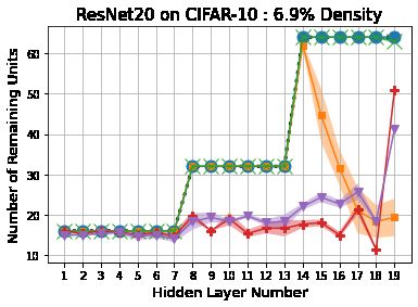
PHEW : Constructing Sparse Networks that Learn Fast and Generalize Well without Training Data

to predict at initialization output changes during training      we conduct a wide range of ablation studies to evaluate the
using the Neural Tangent Kernel (NTK). More recently,            efficacy of PHEW.
(Gebhart et al., 2021) decomposed the NTK into two fac-
tors: one that is only data-dependent, and another that is       2. Background
only architecture-dependent. This decomposition decoupled
the effects of network architecture (including sparsity and      2.1. Neural Tangent Kernel
selection of initial weights) from the effect of training data
                                                                 Let (X , Y) denote the training examples, L the loss func-
on convergence. The architecture-dependent factor can be
                                                                 tion, and f (X , θ) ∈ RN K the network’s output, where N
thought of as the “path covariance” of the network and is
                                                                 is the number of examples and K is the output dimension.
referred to as Path Kernel. The authors of (Gebhart et al.,
                                                                 Under the gradient flow assumption, and denoting the learn-
2021) show that the training convergence of a network can
                                                                 ing rate by η, the output of the network at time t can be
be accurately predicted using the path kernel trace. That
                                                                 approximated using the first-order Taylor expansion,
work concluded with a pruning algorithm (SynFlow-L2) that
designs sparse networks with maximum path kernel trace –               f (X , θ t+1 ) = f (X , θ t ) − η Θt (X , X ) ∇f L   (1)
aiming to optimize at least the architectural component of
the network’s convergence speed.                                 where the matrix Θt (X , X ) = ∇θ f (X , θ t ) ∇θ f (X , θ t )T
In this work, we first show that even though SynFlow and         ∈ RN K×N K is the Neural Tangent Kernel (NTK) at time
Synflow-L2 are optimal in terms of convergence for a given       t (Jacot et al., 2018). Under the additional assumption of
network density, they result in sub-networks with “bottle-       infinite width, the NTK has been shown to remain constant
neck layers” (very small width) – leading to poor perfor-        throughout training, and it allows us to exactly predict the
mance as compared to other data-agnostic methods that use        evolution of the network’s output. More recent work has
the same number of parameters. This issue is observed even       shown that even networks with limited width, and any depth,
at moderate density values. This is expected given the re-       closely follow the NTK dynamics (Lee et al., 2019a). For
cent results of (Golubeva et al., 2021), for instance, showing   a constant NTK Θ0 , and with a mean-squared error loss,
that increasing the width of sparse networks, while keep-        equation (1) has the closed-form solution:
ing the number of parameters constant, generally improves
                                                                    f (X , θ t ) = (I − e−ηΘ0 t )Y + e−ηΘ0 t f (X , θ0 )    (2)
performance.
We then present a method, referred to as PHEW (Paths with        Equation (2) allows us to predict the network’s output given
Higher Edge Weights), which aims to achieve the best of          the input-output training examples, the initial weights θ0 ,
both worlds: high path kernel trace for fast convergence,        and the initial NTK Θ0 . Further, leveraging equation (2), it
and large network width for better generalization perfor-        has been shown that the training convergence is faster in the
mance. Given an unpruned initialized network, and a target       directions that correspond to the larger NTK eigenvalues
number of learnable parameters, PHEW selects a set of            (Arora et al., 2019). This suggests that sparse sub-networks
input-output paths that are conserved in the network and it      that preserve the larger NTK eigenvalues of the original
prunes every remaining connection. The selection of the          network would converge faster and with higher sampling
conserved paths is based strictly on their initial weight val-   efficiency (Wang et al., 2019).
ues – and not on any training data. Further, PHEW induces
randomness into the path selection process using random          2.2. Path kernel decomposition of NTK
walks biased towards higher weight-magnitudes. The net-          More recently, an interesting decomposition of the Neural
work sparsification process does not require any data, and       Tangent Kernel has been proposed that decouples the effects
the pruned network needs to be trained only once.                of the network architecture (and initial weights) from the
We show that selecting paths with higher edge weights forms      data-dependent factors of the training process (Gebhart et al.,
sub-networks that have higher path kernel trace than uniform     2021). We summarize this decomposition next.
random walks – close to the trace obtained through SynFlow-      Consider a neural network f : RD → RK with ReLU
L2. We also show that the use of random walks results            activations, parametrized by θ ∈ Rm . Let P be the set of
in sub-networks having high per-layer width – similar to         all input-output paths, indexed as p = 1, . . . , P (we refer
that of unpruned networks. Further, PHEW avoids layer-           to a path by its index p). Let pi = I{θi ∈ p} represent the
collapse by selecting and conserving input-output paths          presence of edge-weight θi in path p.
instead of individual units or connections. We compare
the performance of PHEW against several pruning before-          The edge-weight-product of a path is defined as Q the prod-
                                                                                                                     m
training methods and show that PHEW achieves significant         uct of edge-weights present in a path, πp (θ) = i=1 θipi .
improvements over SynFlow and SynFlow-L2. Additionally,                   Q variable x, the activation status of a path is,
                                                                 For an input
                                                                 ap (x) = θi ∈p I{zi > 0}, where zi is the activation of the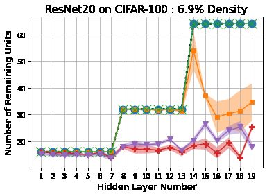
PHEW : Constructing Sparse Networks that Learn Fast and Generalize Well without Training Data

Figure 1. Comparison of the path kernel trace of sparse networks obtained using various pruning methods as well as PHEW.

neuron connected to the previous layer through θi . The k th        training data, the convergence can be effectively approxi-
output of the network can be expressed as:                          mated from the trace of the path kernel:

                        D                                                                   P                   P X
                                                                                                                  m         2
                                                                                 X          X                   X     πp (θ)
                                                                    T r(Πθ ) =       wi =         Πθ (p, p) =                     pi
                        X X
           k
         f (x, θ) =                   πp (θ) ap (x) xi ,      (3)                                                         θi
                        i=1 p∈P i→k                                              i          p=1                 p=1 i=1
                                                                                                                             (6)
where P i→k is the set of paths from input unit i to output         The authors of (Gebhart et al., 2021) empirically validated
unit k. We can now decompose the NTK using the chain                the convergence predicted using the trace of the path kernel
rule:                                                               against the actual training convergence of the network.
                                                                    The previous result has an important consequence for neural
  Θ(X , X ) = ∇π f (X ) ∇θ π(θ) ∇θ π(θ)T ∇π f (X )T
                                                                    network pruning. Given a fully connected neural network
               = Jπf (X ) Jθπ (Jθπ )T Jπf (X )T                     at initialization as well as the target density for a pruned
               = Jπf (X ) Πθ Jπf (X )T                              network, maximizing the path kernel trace of the pruned net-
                                                        (4)         work preserves the largest NTK eigenvalues of the original
The matrix Πθ is referred to as the Path Kernel (Gebhart            network. Since, the directions corresponding to the larger
et al., 2021). The path kernel element for two paths p and          eigenvalues of the NTK learn faster, the sub-network ob-
p0 is:                                                              tained by maximizing the path kernel trace is also expected
                                                                    to converge faster and learn more efficiently.
                       m
                 0
                       X   πp (θ)    πp0 (θ)
       Πθ (p, p ) =                                  pi p0i   (5)   2.3. SynFlow-L1 and SynFlow-L2
                       i=1
                               θi            θi
                                                                    The path kernel framework has been applied in the design
Note that the path kernel, Πθ ∈ RP ×P , depends only on             of pruning algorithms that do not require any training data
the network architecture and the initial weights. On the            (Gebhart et al., 2021; Tanaka et al., 2020). SynFlow-L2
other hand, the matrix Jπf (X ) ∈ RN K×P captures the data-         is such an iterative pruning algorithm that removes edges
dependent activations and re-weights the paths on the basis         (parameters) based on the following saliency function:
of the training data input.
                                                                                                         P         2
                                                                                      ∂R(θ)              X   πp (θ)
                                                                       S(θi ) = θi          = θi                          pi   (7)
Convergence approximation: The eigenstructure of the                                   ∂θi2              p=1
                                                                                                                   θi
NTK depends on how the eigenvectors of Jπf (X ) map onto
the eigenvectors of the path kernel Πθ , as shown by the            The process of computing the previous saliency measure
following result.                                                   and eliminating edges with lower saliency is repeated until
                                                                    the required density is achieved. SynFlow-L2 maximizes
Theorem 1 (Gebhart et al., 2021): Let λi be the eigenval-           the trace of the path kernel, and preserves the following
                                         f
ues of Θ(X , X ), vi the eigenvalues of JP
                                         π (X ) and
                                                  Pwi the           data-independent loss function:
eigenvalues of Πθ . Then λi ≤ vi wi and i λi ≤ i vi wi .                                              !
                                                                                          L+1              P
Given the eigenvalue decomposition of Θ0 , Theorem 1 pro-
                                                                                          Y               X
                                                                                      T         [l] 2
                                                                           R(θ) = 1           |θ | 1 =        (πp (θ))2    (8)
vides an upper bound for the convergence in equation (2).                                   l=1                 p=1
Θ0 with eigenvalues λi has the same eigenvectors as e−ηΘ0 t
                   −ηλi t
                                                                    where |θ [l] |2 is the matrix formed by the squares of the
                                       P
with eigenvalues e        . Therefore, i vi wi accurately
captures the eigenvalues of Θ0 and it can be used to predict        elements of the weight matrix at the lth layer and L is the
the convergence of the training process. Even without any           number of hidden layers.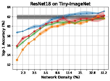
PHEW : Constructing Sparse Networks that Learn Fast and Generalize Well without Training Data

Figure 2. Comparison of the number of remaining units at each layer. The network density is selected such that the method of
Magnitude-Pruning after training is able to achieve within 5% of the unpruned network’s accuracy (see text for justification).

We can also observe empirically in Figure 1 that SynFlow-        Intuitively, the previous results can be justified as follows,
L2 achieves the highest path kernel trace compared to other      with the same weight distribution across all units of a layer,
state-of-the-art pruning methods.                                increasing the number of input-output paths P results in
                                                                 higher path kernel trace. To maximize P with a given num-
Another related pruning method is SynFlow-L1 (or sim-
                                                                 ber of edges m, however, forces the pruning process to only
ply “SynFlow”) – proposed in (Tanaka et al., 2020). Syn-
                                                                 maintain the edges of the smallest possible set of units at
Flow is based on preserving the loss function R(θ) =
PP                                                               each layer. So, the networks produced by SynFlow and
   p=1 |πp (θ)|, which is based on the edge-weight products      SynFlow-L2 tend to have narrower layers, compared to
along each input-output path (rather than their squares).        other pruning methods that do not optimize on the basis of
                                                                 path kernel trace.
3. Pruning for maximum path kernel trace
                                                                 To examine the previous claim empirically, and in the con-
In this section we analyze the resulting architecture of a       text of convolutional networks rather than MLPs, Figure 2
sparse network that has been pruned to maximize the path         compares the number of remaining units at each layer after
kernel trace. As discussed in the previous section, SynFlow-     pruning, using the VGG19 and ResNet20 architectures. The
L2 is a pruning method that has this objective.                  target network density in these experiments is the lowest
                                                                 possible such that the method of Magnitude-Pruning (that
Consider a network with a single hidden-layer, f : RD →          can be performed only after training) achieves within 5%
RD , with N hidden units and D inputs and outputs. The           of the unpruned network’s accuracy. In higher densities
incoming and outgoing weights θ of each unit are initialized     there is still significant redundancy, while in lower densities
by sampling from N (0, 1). Let the number of connections         there is no sufficient capacity to learn the given task. For a
in the unpruned network be M , and let m be the target           convolutional layer, the width of a layer is the number of
number of connections in the pruned network, so that the         channels at the output of that layer. We find that both Syn-
resulting network density is ρ = m/M .                           Flow and SynFlow-L2 result in pruned networks with very
The optimization of the path kernel trace selects the m out      small width (“bottleneck layers”) compared to other state-of-
of M parameters that maximize:                                   the-art pruned networks of the same density.12 Further, with
                  P X  m          2                            SynFlow and SynFlow-L2 all layers have approximately the
                 X          πp (θ)                               same number of remaining units, i.e., approximately equal
                                       pi               (9)
                 p=1 i=1
                              θi                                 width. Note that for the purposes of this analysis (Figure
                                                                 2), we do not include skip connections for ResNet20 – such
In Appendix A.1, we show that this maximization results          connections complicate the definition of “layer width” and
in a fully-connected network in which only n ≤ N of the          paths, but without changing the main result of Figure 2.
hidden-layer units remain in the pruned network – all other
                                                                     1
units and their connections are removed. In other words,               In SNIP, the widest layers get pruned more aggressively as
the network that maximizes the path kernel trace has the nar-    showed in (Tanaka et al., 2020). Due to this SNIP also leads to a
                                                                 decrease in width, but only at the widest layers.
rowest possible hidden-layer width, given a target network           2
                                                                       GraSP and PHEW are able to preserve the same width as the
density.                                                         unpruned network for all the layers. The curves for GraSP (green)
We also show (Appendix A.2) that this network architecture       and PHEW (blue) overlap with the curve for the unpruned network
                                                                 in Figure 2.
maximizes the number of input-output paths P : Given a
target density ρ, the maximum number of paths results when
each hidden-layer has the same number of units, and the
network is fully-connected.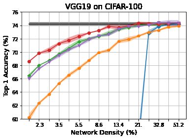
PHEW : Constructing Sparse Networks that Learn Fast and Generalize Well without Training Data

Figure 3. The effect of increasing the layer width of SynFlow and SynFlow-L2 networks, while preserving the same set of param-
eters at each layer. The definition of the x-axis “Width Factor” appears in the main text.

3.1. Effect of network width on performance                       edges of a layer, creating a uniform distribution across all
                                                                  units in the layer – doing so increases the performance of
Several empirical studies have been conducted to under-
                                                                  the network (see Appendix C).
stand the effect of network width and over-parametrization
on learning performance (Neyshabur et al., 2018; Du et al.,      Summary: Let us summarize the observations of this sec-
2018; Park et al., 2019; Lu et al., 2017). However, the previ-   tion regarding the maximization of the path kernel trace –
ous studies do not decouple the effect of increasing width       and the resulting decrease in network width. Even without
from the effect of over-parametrization. Recently, (Gol-         any training data, pruned networks that result by maximiz-
ubeva et al., 2021) examined the effect of network width un-     ing the path kernel trace are expected to converge faster
der a constant number of parameters. That work conducted         and learn more efficiently. As we showed however, for a
experiments with layer-wise random pruning. Starting with        given density, such methods tend to maximize the number
a fully-connected network, the width of each layer is in-        of input-output paths, resulting in pruned networks with
creased while keeping the number of parameters the same.         very narrow layers. Narrow networks, however, attain lower
The experiments of (Golubeva et al., 2021) show that as          performance as compared to wider networks of the same
the network width increases the performance also increases.      layer-wise density. In the next section, we present a method
Further, the distance between the Gaussian kernel formed         that aims to achieve the best of both worlds: high path ker-
by the sparse network and the infinitely wide kernel at ini-     nel trace for fast convergence, and large layer-wise width
tialization is indicative of the network’s performance. As       for better generalization and learning.
expected, increasing the width after a certain limit without
also increasing the number of parameters will inevitably          4. The PHEW network sparsification method
cause a drop in both test and train accuracy because of very
low per-unit connectivity (especially with random pruning).       Given a weight-initialized architecture, and a target number
                                                                  of learnable parameters, we select a set of input-output
We present similar experiments for SynFlow and SynFlow-
                                                                  paths that are conserved in the network – and prune every
L2 in Figure 3. For a given network density, we first obtain
                                                                  connection that does not appear in those paths. The selection
the layer-wise density and number of active units that result
                                                                  of conserved paths is based strictly on their initial weights
from the previous two pruning algorithms. We then gradu-
                                                                 – not on any training data. The proposed method is called
ally increase the number of active units by randomly shuf-
                                                                 ”Paths with Higher Edge Weights” (PHEW) because it has
fling the masks of each layer (so that the number of weights
                                                                  a bias in favor of higher weight connections. Further, the
at each layer is preserved). The increase in layer width can
                                                                  path selection is probabilistic, through biased random walks
be expressed as the fraction x = (w0 − w)/(W − w), where
                                                                  from input units to output units. Specifically, the next-hop
W is the layer width of the unpruned network, w is the layer
                                                                  of each path, from unit i to j at the next layer, is taken with
width in the Synflow (or Synflow-L2) pruned network, and
                                                                  a probability that is proportional to the weight magnitude of
w0 ≥ w is the layer width that results through the shuffling
                                                                  the connection from i to j. We show that conserving paths
method described above. The maximum value x = 1 results
                                                                  with higher edge weight product results in higher path kernel
when w0 = W .
                                                                  trace. The probabilistic nature of PHEW avoids the creation
Figure 3 shows the results of these models on CIFAR-10/100        of ”bottleneck layers” and leads to larger network width
tasks using ResNet20 and VGG19. We can see that as the            than methods with similar path kernel trace. Additionally,
width increases so does the performance of the sparse net-        the procedure of selecting and conserving input-output paths
work, even though the layer-wise number of edges is the           completely avoids layer collapse.
same. Similar results appear in the ablation studies of (Fran-
                                                                  In more detail, let us initially consider a fully-connected
kle et al., 2021) using SynFlow. That study redistributes the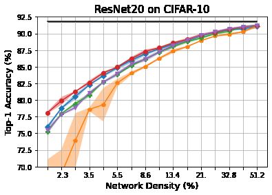
PHEW : Constructing Sparse Networks that Learn Fast and Generalize Well without Training Data

MLP network with L hidden layers and Nl units at each            while there are still connections in other layers (Tanaka
layer (we consider convolutional networks later in this sec-     et al., 2020). Layer collapse causes a disruption of informa-
tion). Suppose that the weights are initialized according to     tion flow through the sparse network making the network
Kaiming’s method (He et al., 2015), i.e., they are sampled       untrainable. SynFlow and SynFlow-L2 have been shown to
from a Normal distribution in which the variance is inversely    avoid layer collapse by iteratively computing gradient based
                                             l
proportional to the width of each layer: θi,j   ∼ N (0, σl2 ),   importance scores and pruning (Tanaka et al., 2020). PHEW
        2                                                        also avoids layer collapse due to its path-based selection and
where σl = 2/Nl .
                                                                 conservation process. Even a single input-output path has
First, let us consider two input-output paths u and b: u         one connection selected at each layer, and so it is impossible
has been selected via a uniform random-walk in which the         for PHEW networks to undergo layer collapse.
probability Q(j, i) that the walk moves from unit i to unit
j at the next layer is the same for all j; b has been selected
                                                                 4.1. Additional PHEW details
via the following weight-biased random-walk process:
                              |θ(j, i)|                          Balanced, bidirectional walks: Without any information
                   Q(j, i) = P                           (10)    about the task or the data, the only reasonable prior is to
                               j |θ(j, i)|
                                                                 assume that every input unit is equally significant – and the
where θ(j, i) is the weight of the connection from i to j.       same for every output unit. For this reason, PHEW attempts
In Appendix A.4 we show that the biased-walk path b con-         to start the same number of walks from each input. And to
tributes more in the path kernel trace than path u:              terminate the same number of walks at each output.

             E[Πθ (b, b)] = 2L × E[Πθ (u, u)]            (11)    To do so, we create paths in both directions with the same
                                                                 probability: forward paths from input units, and reverse
As the number of hidden layers L increases the ratio be-         paths from output units. The selection of the starting unit
tween the two terms becomes exponentially higher. On             in each case is such that the number of walks that start (or
the other hand, as the layer’s width increases the ratio of      terminate) at each input (or output) unit is approximately
two values remains the same. The reason that PHEW paths          the same. The creation of random-walks continues until we
result in higher path kernel trace, compared to the same         have reached the given, target number of parameters.
number of uniformly chosen paths, is that the former tend
to have higher edge weights, and thus higher πp (θ) values       PHEW in convolutional neural networks: A convolu-
(see Equation 6). Empirically, Figure 1 shows that PHEW          tional layer takes as input a 3D-vector with ni channels
achieves a path kernel trace greater than or equal to SNIP       and transforms it into another 3D-vector of ni+1 channels.
and GraSP, and close to the upper bound of SynFlow-L2.           Each of the ni+1 units in a layer produces a single 2D-
                                                                 channel corresponding to the ni+1 channels. A 2D channel
If the PHEW paths were chosen deterministically (say in a        is produced applying convolution on the input vector with ni
greedy manner, always taking the next hop with the highest       channels, using a 3D-filter of depth ni . Therefore each input
weight) the path kernel trace would be slightly higher but the   from a unit at the previous layer has a corresponding 2D-
resulting network would have ”bottlenecks” at the few units      kernel as one of the channels in the filter. So, even though
that have the highest incoming weights. PHEW avoids this         MLPs have an individual weight per edge, convolutional
problem by introducing randomness in the path selection          networks have a 2D-kernel per edge.
process. Specifically, in Appendix A.3 we show that the
expected number of random walks through each unit of a           A random-walk can traverse an edge of a convolutional
layer l is W/Nl , where W is the required number of walks        network in two ways: either traversing a single weight in
to achieve the target network density. Thus, as long as          the corresponding 2D kernel – or traversing the entire kernel
W > Nl , every unit is expected to be traversed by at least      with all its weights. Traversing a single weight from a kernel
one walk – and thus every unit of that layer is expected to      conserves that edge and produces a non-zero output channel.
be present in the sparsified network.                            This creates sparse kernels and allows for the processing
                                                                 of multiple input channels at the same unit and with fewer
This is very different than the behavior of SynFlow or           parameters. On the other hand, traversing the entire 2D-
SynFlow-L2, in which the width of several layers in the          kernel that corresponds to an edge means that several other
pruned network is significantly reduced. Empirically, Fig-       kernels will be eliminated. Earlier work in pruning has
ure 2 confirms that PHEW achieves the larger per-layer           shown empirically the higher performance of creating sparse
width, compared to SynFlow and SynFlow-L2. Addition-             kernels instead of pruning entire kernels (Blalock et al.,
ally, the per-layer width remains the same as the width of       2020; Liu et al., 2019). Therefore, in PHEW we choose
the original unpruned network.                                   to conserve individual parameters during a random-walk
Layer-Collapse: Layer collapse is defined as a network           rather than conserving entire kernels.
state in which all edges of a specific layer are eliminated,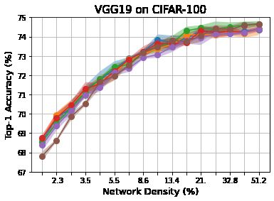
PHEW : Constructing Sparse Networks that Learn Fast and Generalize Well without Training Data
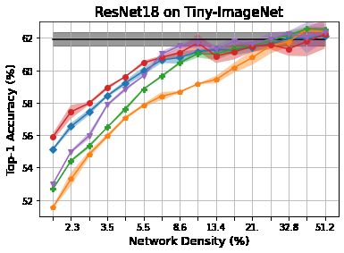
Figure 4. Comparison of the Top-1 accuracy for sparse networks obtained using PHEW and other state-of-the-art data-
independent baselines. The mean is shown as a solid line while the standard deviation is shown as shaded area.
In summary, PHEW follows a two-step process in convolu- with SynFlow and SynFlow-L2, which also do not require
tional networks: first an edge (i.e., 2D-kernel) is selected any training data.
using equation (10). Then a single weight is chosen from
We present results for three networks: ResNet20, VGG19
that kernel, randomly, with a probability that is proportional
and ResNet18 – and three datasets: CIFAR-10, CIFAR-100
to the weight of the sampled parameter. We have also exper-
and Tiny ImageNet. The network density range is chosen
imented with the approach of conserving the entire kernel,
such that the magnitude pruning after training method (our
and we also present results for that case in the next section.
performance upper bound) maintains a comparable accuracy
to the unpruned network. We claim that it is not important in
5. Experimental results practice to consider densities in which any pruned network
would perform poorly. The hyper-parameters used were
In this section we present several experiments conducted to
tuned only for the unpruned network (see Appendix D). We
compare the performance of PHEW against state-of-the-art
run each experiment three times for different seed values
pruning methods and other baselines. We present results
and present the mean and standard deviation of the test
both for standard image classification tasks using convolu-
accuracy.
tional networks as well as an image-transformation task us-
ing MLPs (that task is described in more detail in Appendix Data-independent methods: We first compare PHEW
B). We also conduct a wide variety of ablation studies to against data-independent pruning baselines random prun-
test the efficacy of PHEW. ing, initial magnitude pruning, and methods SynFlow and
SynFlowL2 in Figure 4. At the density levels considered,
5.1. Classification comparisons PHEW performs better than both SynFlow and SynFlow-L2.
We attribute this superior performance to the large per-layer
We compare PHEW against two baselines, Random pruning width of the sparse networks obtained through PHEW. As
and Initial (Weight) Magnitude pruning, along with four we showed earlier, differences in layer-wise width of sparse
state-of-the-art algorithms: SNIP (Lee et al., 2019b), GraSP networks accounts for most of the performance differences,
(Wang et al., 2019), SynFlow (Tanaka et al., 2020) and under the same number of parameters. Further, the perfor-
SynFlow-L2 (Gebhart et al., 2021). We also present results mance gap increases for datasets with more classes, such as
for the original Unpruned network as well as for Gradual Tiny-ImageNet as compared to CIFAR-10 and CIFAR-100.
Magnitude Pruning (Zhu & Gupta, 2017) to upper bound We believe that this is due to the increased complexity of
the network’s performance for a given density. Because the dataset and the need for larger width to learn finer and
PHEW is data-independent, the most relevant comparison is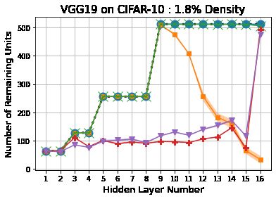
PHEW : Constructing Sparse Networks that Learn Fast and Generalize Well without Training Data

Figure 5. Comparison of the Top-1 accuracy for sparse networks obtained using PHEW and other state-of-the-art data-dependent
pruning methods and baselines. The mean is shown as a solid line while the standard deviation is shown as shaded area.

disconnected decision regions (Nguyen et al., 2018).
Data-dependent methods: Figure 5 compares the test ac-
curacy of PHEW networks against various data-dependent
pruning algorithms. It is interesting that PHEW outperforms
in many cases the data-dependent pruning algorithms GraSP
and SNIP even though it is agnostic to the data or task.
At higher network densities, PHEW is competitive with
SNIP. Note that SNIP also utilizes paths with higher weight
magnitudes (Gebhart et al., 2021). At lower network den-
                                                                  Figure 6. Ablation Studies: Comparison of several sparse networks
sities, SNIP’s accuracy falls quickly while the accuracy
                                                                  obtained using variants of PHEW.
of PHEW falls more gradually creating a significant gap.
This is because SNIP eliminates units at a higher rate at
the largest layer (Figure 2), which eventually leads to layer
collapse (Tanaka et al., 2020).                                   5.2. Ablation Studies
GraSP on the other hand is competitive with PHEW at lower         In this section we conduct a wide variety of ablation studies
density levels and falls short of PHEW at moderate and            to test PHEW’s efficacy as well as to understand fully the
higher network densities. This is because GraSP maximizes         cause behind its generalization performance.
gradient flow after pruning, and the obstruction to gradient
flow is prominent only at lower density levels. Further, it has   Kernel-conserved PHEW variant: We study a PHEW
been shown that GraSP performs better than SNIP only at           variant for convolutional neural networks where instead of
lower density levels (Wang et al., 2019), which is consistent     conserving a single weight of a kernel each time a random
with our observations.                                            walk traverses that kernel, we conserve the entire kernel.
                                                                  This approach reduces the FLOP count immensely by elimi-
PHEW is able to perform relatively well across all density        nating the operations performed on several 2D feature maps
levels. At lower density levels, the obstruction to the flow      in specific units. We present the comparison for CIFAR10
of gradients is avoided by conserving input-output paths.         and CIFAR100 in Figure 6. Note that at moderate network
Further, by selecting higher weight magnitudes, PHEW              densities, this kernel-conserved variant performs as well as
avoids the problem of vanishing gradients.                        the other methods we consider – therefore this variant can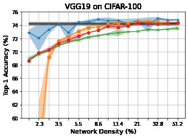
PHEW : Constructing Sparse Networks that Learn Fast and Generalize Well without Training Data

                                                                     We present results for three reinitialization schemes, a)
                                                                     dense reinitialization, b) layer-wise sparse reinitialization
                                                                     (Liu et al., 2019) and c) neuron-wise sparse reinitialization
                                                                     (Evci et al., 2020).
                                                                     We observe that reinitialized PHEW networks also achieve
                                                                     the same performance as the original PHEW network.
                                                                     This further confirms that the sparse architecture produced
                                                                     through the random walk process is sufficient to obtain
                                                                     PHEW’s generalization performance.

Figure 7. Comparison of PHEW against random pruning with             In Figure 7 we also compare with reinitialized randomly
sparse initialization and reinitialized PHEW networks. PHEW          pruned networks, as those networks have been shown to
variants are concentrated at the upper part of plots, while random   improve performance. Although we see some improvements
pruning variants are concentrated at the lower part.                 with sparse reinitialization in randomly pruned networks,
                                                                     the performance still falls short of PHEW and its variants.

be utilized when decreasing the FLOP count is a priority.
                                                                     6. Conclusion
Different weight initializations: PHEW depends on initial
weights, and so it is important to examine the robustness            We proposed a probabilistic approach called PHEW to con-
of PHEW’s performance across the major weight initializa-            struct sparse networks without any training data. Sparse
tion methods used in practice: Kaiming ((He et al., 2015)),          networks that result by maximizing the path kernel trace are
Normal N (0, 0.1), and Xavier uniform ((Glorot & Bengio,             expected to converge faster. We showed that, for a given
2010)). Figure 6 shows results with such initializations for         density, methods that maximize the path kernel trace result
VGG19 and ResNet20 on CIFAR10 and CIFAR100. Note                     in very narrow layers and lower performance compared to
that PHEW’s performance is quite robust across all these             wider networks of the same layer-wise density. On the other
weight initializations. It is interesting that PHEW’s perfor-        hand, conserving paths with higher edge-weight magnitudes
mance is not altered by initializing all layers with the same        leads to sparse networks with higher path kernel trace. Fur-
distribution. This may be due to the random walk proce-              ther, introducing randomness in the path selection process
dure, where the probability distribution at each hop is only         preserves the layer-wise width of the unpruned network.
dependent on the initial weights of that layer.                      Empirically, we showed that PHEW achieves significant im-
                                                                     provements over current data-independent state-of-the-art
Unbiased and “inverse-weight biased” random walks:                   pruning at initialization methods.
We also present two variants of PHEW: a) unbiased (uni-
form) walks, and b) random walks that are biased in favor of         Some open questions for future research are: 1) A compari-
lower weight-magnitudes. The former selects the next-hop             son between PHEW networks and “winning tickets” (Fran-
of the walk randomly, ignoring the weights, while the latter         kle & Carbin, 2018), given the same number of parameters,
gives higher probability to lower weight-connections.                both in terms of their convergence speed and structural prop-
                                                                     erties. 2) Development of path-based network sparsification
The two variants perform similar with PHEW in terms of               methods that can utilize a limited amount of training data to
accuracy, as shown in Figure 6, because they create networks         get even higher performance than PHEW. 3) How to iden-
that have the same per-layer width with PHEW.                        tify path-based sparse networks that can perform as well
Their difference with PHEW is in terms of convergence                as PHEW networks but without any training? 4) How to
speed. The reason is that they are not biased in favor of            dynamically determine the optimal number of parameters in
higher-weight connections, and so the resulting path kernel          a sparse network at the early stages of training – instead of
trace is lower than that in PHEW. Indeed, we have also               starting with a pre-determined target number of parameters?
confirmed empirically that the training error drops faster
initially (say between epochs 1 to 20) in PHEW than in               Acknowledgements
these two variants.
                                                                     This work is supported by the National Science Foundation
Re-initializing PHEW Networks: We have also con-                     (Award: 2039741) and by the Lifelong Learning Machines
ducted experiments with reinitialized sparse networks se-            (L2M) program of DARPA/MTO (Cooperative Agreement
lected through PHEW. Here, the architecture of the sparse            HR0011-18-2-0019). The authors acknowledge the con-
network remains the same but the individual weights are              structive comments given by the ICML and ICLR 2021
re-sampled. This causes the path-kernel trace to be lower            reviewers and by Cameron Taylor.
while the architecture produced by PHEW is maintained.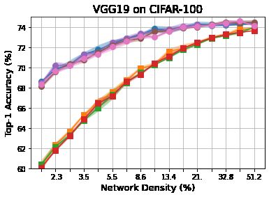
PHEW : Constructing Sparse Networks that Learn Fast and Generalize Well without Training Data

References                                                       Golubeva, A., Gur-Ari, G., and Neyshabur, B. Are wider
                                                                   nets better given the same number of parameters? In
Arora, S., Du, S., Hu, W., Li, Z., and Wang, R. Fine-grained
                                                                  International Conference on Learning Representations,
  analysis of optimization and generalization for overpa-
                                                                   2021. URL https://openreview.net/forum?
  rameterized two-layer neural networks. In International
                                                                   id=_zx8Oka09eF.
  Conference on Machine Learning, pp. 322–332. PMLR,
  2019.                                                          Guo, Y., Yao, A., and Chen, Y. Dynamic network surgery
                                                                   for efficient dnns. In Advances in neural information
Blalock, D., Ortiz, J. J. G., Frankle, J., and Guttag, J. What
                                                                   processing systems, pp. 1379–1387, 2016.
  is the state of neural network pruning? arXiv preprint
  arXiv:2003.03033, 2020.                                        Han, S., Mao, H., and Dally, W. J. Deep compres-
                                                                   sion: Compressing deep neural networks with pruning,
Carreira-Perpinán, M. A. and Idelbayev, Y. “learning-             trained quantization and huffman coding. arXiv preprint
  compression” algorithms for neural net pruning. In Pro-          arXiv:1510.00149, 2015a.
  ceedings of the IEEE Conference on Computer Vision
  and Pattern Recognition, pp. 8532–8541, 2018.                  Han, S., Pool, J., Tran, J., and Dally, W. Learning both
                                                                   weights and connections for efficient neural network. In
Dong, X., Chen, S., and Pan, S. Learning to prune deep            Advances in neural information processing systems, pp.
  neural networks via layer-wise optimal brain surgeon. In        1135–1143, 2015b.
 Advances in Neural Information Processing Systems, pp.
 4857–4867, 2017.                                                Hassibi, B. and Stork, D. G. Second order derivatives for
                                                                   network pruning: Optimal brain surgeon. In Advances
Du, S. S., Zhai, X., Poczos, B., and Singh, A. Gradient            in neural information processing systems, pp. 164–171,
  descent provably optimizes over-parameterized neural            1993.
  networks. arXiv preprint arXiv:1810.02054, 2018.
                                                                 He, K., Zhang, X., Ren, S., and Sun, J. Delving deep
Evci, U., Ioannou, Y. A., Keskin, C., and Dauphin, Y. Gradi-       into rectifiers: Surpassing human-level performance on
  ent flow in sparse neural networks and how lottery tickets       imagenet classification. In Proceedings of the IEEE inter-
  win. arXiv preprint arXiv:2010.03533, 2020.                      national conference on computer vision, pp. 1026–1034,
                                                                   2015.
Frankle, J. and Carbin, M. The lottery ticket hypothesis:
  Finding sparse, trainable neural networks. In Interna-         He, K., Zhang, X., Ren, S., and Sun, J. Deep residual learn-
  tional Conference on Learning Representations, 2018.             ing for image recognition. In Proceedings of the IEEE
                                                                   conference on computer vision and pattern recognition,
Frankle, J., Dziugaite, G. K., Roy, D. M., and Carbin, M.
                                                                   pp. 770–778, 2016.
  Stabilizing the lottery ticket hypothesis. arXiv preprint
  arXiv:1903.01611, 2019.                                        Jacot, A., Gabriel, F., and Hongler, C. Neural tangent kernel:
                                                                   Convergence and generalization in neural networks. In
Frankle, J., Dziugaite, G. K., Roy, D., and Carbin, M. Linear      Advances in neural information processing systems, pp.
  mode connectivity and the lottery ticket hypothesis. In          8571–8580, 2018.
  International Conference on Machine Learning, pp. 3259–
  3269. PMLR, 2020.                                              Janowsky, S. A. Pruning versus clipping in neural networks.
                                                                   Physical Review A, 39(12):6600, 1989.
Frankle, J., Dziugaite, G. K., Roy, D., and Carbin, M. Prun-
  ing neural networks at initialization: Why are we missing      Karnin, E. D. A simple procedure for pruning back-
  the mark? In International Conference on Learning                propagation trained neural networks. IEEE transactions
  Representations, 2021. URL https://openreview.                   on neural networks, 1(2):239–242, 1990.
  net/forum?id=Ig-VyQc-MLK.
                                                                 LeCun, Y., Denker, J. S., and Solla, S. A. Optimal brain
Gebhart, T., Saxena, U., and Schrater, P. A unified paths          damage. In Advances in neural information processing
  perspective for pruning at initialization. arXiv preprint        systems, pp. 598–605, 1990.
  arXiv:2101.10552, 2021.
                                                                 Lee, J., Xiao, L., Schoenholz, S., Bahri, Y., Novak, R., Sohl-
Glorot, X. and Bengio, Y. Understanding the difficulty             Dickstein, J., and Pennington, J. Wide neural networks of
  of training deep feedforward neural networks. In Pro-            any depth evolve as linear models under gradient descent.
  ceedings of the thirteenth international conference on           In Advances in neural information processing systems,
  artificial intelligence and statistics, pp. 249–256, 2010.       pp. 8572–8583, 2019a.
PHEW : Constructing Sparse Networks that Learn Fast and Generalize Well without Training Data
Lee, N., Ajanthan, T., and Torr, P. SNIP: SINGLE- 2020. URL https://openreview.net/forum?
SHOT NETWORK PRUNING BASED ON CONNEC- id=ryl3ygHYDB.
TION SENSITIVITY. In International Conference on
Learning Representations, 2019b. URL https:// Russakovsky, O., Deng, J., Su, H., Krause, J., Satheesh, S.,
openreview.net/forum?id=B1VZqjAcYX. Ma, S., Huang, Z., Karpathy, A., Khosla, A., Bernstein,
M., et al. Imagenet large scale visual recognition chal-
Liu, Z., Sun, M., Zhou, T., Huang, G., and Darrell, lenge. International journal of computer vision, 115(3):
T. Rethinking the value of network pruning. In In- 211–252, 2015.
ternational Conference on Learning Representations,
2019. URL https://openreview.net/forum? Simonyan, K. and Zisserman, A. Very deep convolu-
id=rJlnB3C5Ym. tional networks for large-scale image recognition. arXiv
preprint arXiv:1409.1556, 2014.
Lu, Z., Pu, H., Wang, F., Hu, Z., and Wang, L. The expres-
sive power of neural networks: a view from the width. Tanaka, H., Kunin, D., Yamins, D. L., and Ganguli, S. Prun-
In Proceedings of the 31st International Conference on ing neural networks without any data by iteratively con-
Neural Information Processing Systems, pp. 6232–6240, serving synaptic flow. Advances in Neural Information
2017. Processing Systems, 33, 2020.
Molchanov, P., Mallya, A., Tyree, S., Frosio, I., and Kautz, Wang, C., Zhang, G., and Grosse, R. Picking winning
J. Importance estimation for neural network pruning. In tickets before training by preserving gradient flow. In
Proceedings of the IEEE Conference on Computer Vision International Conference on Learning Representations,
and Pattern Recognition, pp. 11264–11272, 2019a. 2019.
Molchanov, P., Tyree, S., Karras, T., Aila, T., and Kautz, You, H., Li, C., Xu, P., Fu, Y., Wang, Y., Chen, X., Bara-
J. Pruning convolutional neural networks for resource niuk, R. G., Wang, Z., and Lin, Y. Drawing early-bird
efficient inference. In 5th International Conference on tickets: Toward more efficient training of deep networks.
Learning Representations, ICLR 2017-Conference Track In International Conference on Learning Representations,
Proceedings, 2019b. 2019.
Morcos, A., Yu, H., Paganini, M., and Tian, Y. One ticket Yu, R., Li, A., Chen, C.-F., Lai, J.-H., Morariu, V. I., Han,
to win them all: generalizing lottery ticket initializations X., Gao, M., Lin, C.-Y., and Davis, L. S. Nisp: Pruning
across datasets and optimizers. In Advances in Neural networks using neuron importance score propagation. In
Information Processing Systems, pp. 4932–4942, 2019. Proceedings of the IEEE Conference on Computer Vision
and Pattern Recognition, pp. 9194–9203, 2018.
Mozer, M. C. and Smolensky, P. Skeletonization: A tech-
nique for trimming the fat from a network via relevance Zhu, M. and Gupta, S. To prune, or not to prune: exploring
assessment. In Advances in neural information process- the efficacy of pruning for model compression. arXiv
ing systems, pp. 107–115, 1989. preprint arXiv:1710.01878, 2017.
Neyshabur, B., Li, Z., Bhojanapalli, S., LeCun, Y., and
Srebro, N. The role of over-parametrization in general-
ization of neural networks. In International Conference
on Learning Representations, 2018.
Nguyen, Q., Mukkamala, M. C., and Hein, M. Neural
networks should be wide enough to learn disconnected
decision regions. In International Conference on Machine
Learning, pp. 3740–3749. PMLR, 2018.
Park, D., Sohl-Dickstein, J., Le, Q., and Smith, S. The ef-
fect of network width on stochastic gradient descent and
generalization: an empirical study. In International Con-
ference on Machine Learning, pp. 5042–5051. PMLR,
2019.
Park*, S., Lee*, J., Mo, S., and Shin, J. Lookahead: A
far-sighted alternative of magnitude-based pruning. In
International Conference on Learning Representations,You can also read