VarAFT Documentation Jean-Pierre Desvignes, David Salgado - April 29, 2019
←
→
Page content transcription
If your browser does not render page correctly, please read the page content below
VarAFT Documentation
    Jean-Pierre Desvignes, David Salgado
Aix-Marseille University - INSERM U 1251 Genetics and Bioinformatics Team

                           April 29, 2019

                                   1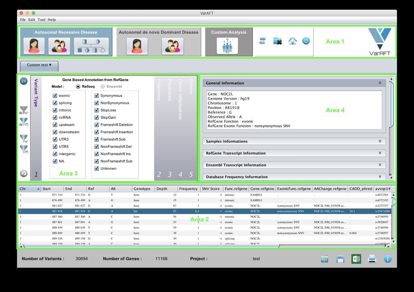
Contents
1 Introduction                                                                                                                                                         3

2 Installation                                                                                                                                                         3
  2.1 Windows . . . . . . . . . . . . . . . . . . . . . . . . . . . . . . . . . . . . . . . . .                                                                        4
  2.2 MAC . . . . . . . . . . . . . . . . . . . . . . . . . . . . . . . . . . . . . . . . . . . .                                                                      4
  2.3 UNIX . . . . . . . . . . . . . . . . . . . . . . . . . . . . . . . . . . . . . . . . . . .                                                                       5

3 Settings                                                                                                                                                             7
  3.1 General . . . . . . . . . . . . .           .   .   .   .   .   .   .   .   .   .   .   .   .   .   .   .   .   .   .   .   .   .   .   .   .   .   .   .   .    7
  3.2 VCF . . . . . . . . . . . . . . .           .   .   .   .   .   .   .   .   .   .   .   .   .   .   .   .   .   .   .   .   .   .   .   .   .   .   .   .   .    8
  3.3 Annotation . . . . . . . . . . .            .   .   .   .   .   .   .   .   .   .   .   .   .   .   .   .   .   .   .   .   .   .   .   .   .   .   .   .   .    9
  3.4 Tools . . . . . . . . . . . . . . .         .   .   .   .   .   .   .   .   .   .   .   .   .   .   .   .   .   .   .   .   .   .   .   .   .   .   .   .   .   10
       3.4.1 UMD-Predictor . . . . .              .   .   .   .   .   .   .   .   .   .   .   .   .   .   .   .   .   .   .   .   .   .   .   .   .   .   .   .   .   10
       3.4.2 Human Splicing Finder                .   .   .   .   .   .   .   .   .   .   .   .   .   .   .   .   .   .   .   .   .   .   .   .   .   .   .   .   .   11
  3.5 Table content . . . . . . . . . .           .   .   .   .   .   .   .   .   .   .   .   .   .   .   .   .   .   .   .   .   .   .   .   .   .   .   .   .   .   12
  3.6 Versionning . . . . . . . . . . .           .   .   .   .   .   .   .   .   .   .   .   .   .   .   .   .   .   .   .   .   .   .   .   .   .   .   .   .   .   14

4 Annotation Tool                                                                                                                                                     16
  4.1 Variant Files Annotation .      .   .   .   .   .   .   .   .   .   .   .   .   .   .   .   .   .   .   .   .   .   .   .   .   .   .   .   .   .   .   .   .   17
  4.2 UMD-Predictor . . . . . .       .   .   .   .   .   .   .   .   .   .   .   .   .   .   .   .   .   .   .   .   .   .   .   .   .   .   .   .   .   .   .   .   20
  4.3 Human Splicing Finder . .       .   .   .   .   .   .   .   .   .   .   .   .   .   .   .   .   .   .   .   .   .   .   .   .   .   .   .   .   .   .   .   .   21
  4.4 Manage Database . . . . .       .   .   .   .   .   .   .   .   .   .   .   .   .   .   .   .   .   .   .   .   .   .   .   .   .   .   .   .   .   .   .   .   23
      4.4.1 Download dbSNP            .   .   .   .   .   .   .   .   .   .   .   .   .   .   .   .   .   .   .   .   .   .   .   .   .   .   .   .   .   .   .   .   24
      4.4.2 Create DBLocal .          .   .   .   .   .   .   .   .   .   .   .   .   .   .   .   .   .   .   .   .   .   .   .   .   .   .   .   .   .   .   .   .   26

5 Analysis and filter tool                                                                                                                                            28
  5.1 Manual Filtering . . . . . .        .   .   .   .   .   .   .   .   .   .   .   .   .   .   .   .   .   .   .   .   .   .   .   .   .   .   .   .   .   .   .   29
      5.1.1 Mode of inheritance           .   .   .   .   .   .   .   .   .   .   .   .   .   .   .   .   .   .   .   .   .   .   .   .   .   .   .   .   .   .   .   31
      5.1.2 Filtration area . . .         .   .   .   .   .   .   .   .   .   .   .   .   .   .   .   .   .   .   .   .   .   .   .   .   .   .   .   .   .   .   .   43
      5.1.3 Others . . . . . . . .        .   .   .   .   .   .   .   .   .   .   .   .   .   .   .   .   .   .   .   .   .   .   .   .   .   .   .   .   .   .   .   54
      5.1.4 Variant Informations          .   .   .   .   .   .   .   .   .   .   .   .   .   .   .   .   .   .   .   .   .   .   .   .   .   .   .   .   .   .   .   55
      5.1.5 Result table . . . . .        .   .   .   .   .   .   .   .   .   .   .   .   .   .   .   .   .   .   .   .   .   .   .   .   .   .   .   .   .   .   .   59
      5.1.6 Other Options . . .           .   .   .   .   .   .   .   .   .   .   .   .   .   .   .   .   .   .   .   .   .   .   .   .   .   .   .   .   .   .   .   60
  5.2 Automatic Filtering . . . .         .   .   .   .   .   .   .   .   .   .   .   .   .   .   .   .   .   .   .   .   .   .   .   .   .   .   .   .   .   .   .   61

6 Coverage Analysis                                                                                                                                                   65
  6.1 Compute Coverage . . . . . . . . . . . . . . . . . . . . . . . . . . . . . . . . . . . .                                                                        66
  6.2 Show Coverage . . . . . . . . . . . . . . . . . . . . . . . . . . . . . . . . . . . . . .                                                                       68
  6.3 Create BED . . . . . . . . . . . . . . . . . . . . . . . . . . . . . . . . . . . . . . . .                                                                      74

7 Other                                                                                                                                                               74
  7.1 Gene list . . . . . . . . . . . . . . . . . . . . . . . . . . . . . . . . . . . . . . . . . .                                                                   74

                                                                  1
8 Version History                                                                                                                                                   76
  8.1 2.16 : April 30, 2019 . . . .     .   .   .   .   .   .   .   .   .   .   .   .   .   .   .   .   .   .   .   .   .   .   .   .   .   .   .   .   .   .   .   76
  8.2 2.15.1 : March 19, 2019 . .       .   .   .   .   .   .   .   .   .   .   .   .   .   .   .   .   .   .   .   .   .   .   .   .   .   .   .   .   .   .   .   77
  8.3 2.15.1 : March 08, 2019 . .       .   .   .   .   .   .   .   .   .   .   .   .   .   .   .   .   .   .   .   .   .   .   .   .   .   .   .   .   .   .   .   77
  8.4 2.15 : January 4th, 2018 . .      .   .   .   .   .   .   .   .   .   .   .   .   .   .   .   .   .   .   .   .   .   .   .   .   .   .   .   .   .   .   .   78
  8.5 2.14 : September 17, 2018 .       .   .   .   .   .   .   .   .   .   .   .   .   .   .   .   .   .   .   .   .   .   .   .   .   .   .   .   .   .   .   .   79
  8.6 2.13 : April 20, 2018 . . . .     .   .   .   .   .   .   .   .   .   .   .   .   .   .   .   .   .   .   .   .   .   .   .   .   .   .   .   .   .   .   .   81
  8.7 2.12.1 : March 07, 2018 . .       .   .   .   .   .   .   .   .   .   .   .   .   .   .   .   .   .   .   .   .   .   .   .   .   .   .   .   .   .   .   .   82
  8.8 2.12 : February 05, 2018 . .      .   .   .   .   .   .   .   .   .   .   .   .   .   .   .   .   .   .   .   .   .   .   .   .   .   .   .   .   .   .   .   82
  8.9 2.11.1 : October 05, 2017 .       .   .   .   .   .   .   .   .   .   .   .   .   .   .   .   .   .   .   .   .   .   .   .   .   .   .   .   .   .   .   .   84
  8.10 2.11 : October 03, 2017 . .      .   .   .   .   .   .   .   .   .   .   .   .   .   .   .   .   .   .   .   .   .   .   .   .   .   .   .   .   .   .   .   84
  8.11 2.10.2 : September 06, 2017      .   .   .   .   .   .   .   .   .   .   .   .   .   .   .   .   .   .   .   .   .   .   .   .   .   .   .   .   .   .   .   85
  8.12 2.10.1 : August 25 , 2017 .      .   .   .   .   .   .   .   .   .   .   .   .   .   .   .   .   .   .   .   .   .   .   .   .   .   .   .   .   .   .   .   85
  8.13 2.10 : August 2017 . . . . .     .   .   .   .   .   .   .   .   .   .   .   .   .   .   .   .   .   .   .   .   .   .   .   .   .   .   .   .   .   .   .   86
  8.14 2.06 : February 2017 . . . .     .   .   .   .   .   .   .   .   .   .   .   .   .   .   .   .   .   .   .   .   .   .   .   .   .   .   .   .   .   .   .   87
  8.15 2.05 : November 2016 . . .       .   .   .   .   .   .   .   .   .   .   .   .   .   .   .   .   .   .   .   .   .   .   .   .   .   .   .   .   .   .   .   88
  8.16 2.04 : August 2016 . . . . .     .   .   .   .   .   .   .   .   .   .   .   .   .   .   .   .   .   .   .   .   .   .   .   .   .   .   .   .   .   .   .   90
  8.17 2.01 to 2.03 . . . . . . . . .   .   .   .   .   .   .   .   .   .   .   .   .   .   .   .   .   .   .   .   .   .   .   .   .   .   .   .   .   .   .   .   91
  8.18 2.00 : June 2016 . . . . . .     .   .   .   .   .   .   .   .   .   .   .   .   .   .   .   .   .   .   .   .   .   .   .   .   .   .   .   .   .   .   .   92

9 Frequently asked questions                                                                                                                                        94

10 Contact us                                                                                                                                                       94

                                                                2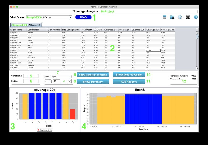
Figure 1: Main Menu of VarAFT

1    Introduction
VarAFT (Variant Annotation and Filter Tool) is a tool used to annotate and filter out variant
files. VarAFT allows the comparison of several individuals and the collection of relevant information
about variations. A direct link to IGV is available to visualize any variations using a ’BAM’ file.
VarAFT includes a coverage analysis module to easily visualize regions that are poorly covered
through tables and dynamic charts.

2    Installation
VarAFT is available for Linux, Mac and Windows.

                                                 3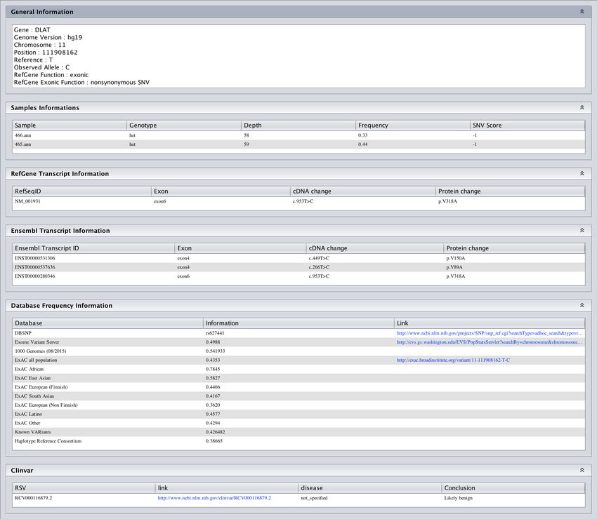
WARNING
   JAVA version 1.8 64-bits is necessary.
   The OpenJDK version of JAVA is not supported. VarAFT could be launched with JAVA
   9 or higher.

2.1   Windows
For the first installation, you should use the "VarAFT_Setup_First_Install.exe" file to install
’VarAFT ’, ’Perl’, ’Annovar’, ’IGV ’ and ’BEDtools’. If you want to update VarAFT, you should
use the "VarAFT_Setup.exe" file.
   If you have no administrator rights, you can download the "no admin rights’ version. This
version will setup VarAFT in your user folder.
   After a successful installation, the program can be started using the VarAFT.exe file.
   NOTE

   By default the tool utilize 4GB of RAM (basic configuration for a recent desktop com-
   puter). If you have a 32-bits Windows OS and less than 3GB of RAM, you must launch
   "C:\\Program Files (x86)\VarAFT_min.exe" to start VarAFT. To use more memory you
   can launch VarAFT with the VarAFT_8G.exe, VarAFT_16G.exe or VarAFT_32G.exe.

2.2   MAC
Download the ".pkg" file for MAC OS. Double click on the file. Accept the license and follow
instructions. Wait until the copy finish. VarAFT will be available in your "Applications" folder.

                           Figure 2: Installation of VarAFT on MAC

                                               4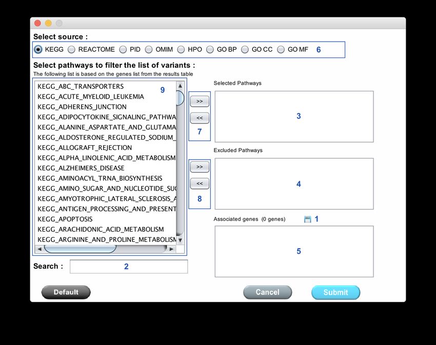
VarAFT was built to use 8Gb of authorized max RAM . To change this value you can modify
this file : "/Applications/VarAFT.app/Contents/Java/VarAFT.cfg".

  sudo v i / A p p l i c a t i o n s /VarAFT . app/ Contents / Java /VarAFT . c f g

 [ JVMUserOptions ]
 −Xmx=8192m
cd path_to_my_varaft_rpm_package
  sudo yum i n s t a l l v a r a f t −2.13 −1. x86_64 . rpm

   VarAFT was built to be launched with 8Gb of authorized max RAM . To change this value
you can edit this file : "/opt/VarAFT/app/VarAFT.cfg".

  sudo v i / opt /VarAFT/app/VarAFT . c f g

 [ JVMUserOptions ]
 −Xmx=8192m
3     Settings
VarAFT standard settings can be edited and adjusted to your needs.

                          Figure 3: Settings Panel to configure VarAFT

3.1    General
    • Path to IGV: Select the path of IGV tool. IGV allows visualization of BAM files. By
      default IGV is provided within VarAFT and the path is automatically set during the initial
      installation.
    • Path to Annovar database: Select the directory where you want to store all needed files
      for the annotation process. These files need at least 50gb to be all downloaded. Please make
      sure you have enough free space in your computer. By default Annovar database is stored in
      your user folder.
    • Path to VarAFT_Project: Select the directory where you want to store your projects.
      By default the folder VarAFT_Project is stored in your user folder.

                                                7
• Path to dblocal default file: Select the path of your local database. A specific VarAFT
     module allows for generation of this file from your VCF files.
   • Number of thread allowed: Set the max number of allowed threads for annotation and
     coverage analysis. Please check your performance computer before changing this value. Note
     that you have less than 3gb of ram or a 32-bit system, it is advised to set this parameter to
     1. An optimal value is the total number of cores - 2.

3.2   VCF
This section allows the configuration of VarAFT for the conversion of the VCF file.

                Figure 4: Settings Panel to configure VarAFT : VCF conversion

   • 1 Variants with an allele frequency lower than this value are considered as reference homozy-
     gous and are excluded from the analysis.

         NOTE
         Set 0 to keep all variants for example in the case of mosaicism or somatic events.

                                                8
• 2 Variants with an allele frequency greater than this value are considered as homozygous.
  • 3 Variants with an allele frequency greater than the first value and lower than the second
    are considered as heterozygous. Variants with an allele frequency lower than the first value
    (and greater than value of part 1) will be considered as uncertain heterozygous.

3.3   Annotation

                 Figure 5: Settings panel to configure VarAFT : Annotation

  This section allows the configuration of VarAFT for the annotation process.

  • 1 Check this box if you want to download and use KAVIAR database.
  • 2 Check this box if you want to download and use HRCR1 database.
  • 3 Check this box if you want to download and use gnomAD Genome database. gnomAD
    exome is automatically used.
  • 4 Check this box if you want to download and use the Great Midddle East database.
  • 5 Check this box if you want to download and use Iranome Database.

                                              9
• 6 Set the distance between splicing variants and exon/intron boundaries. These variants will
be flagged as splicing instead of intronic.
• 7 Check this box if you want to get all possible types of variants for all transcripts. By
default only the most relevant type is displayed.
3.4 Tools
Figure 6: Settings panel to configure VarAFT : Tools
VarAFT uses API from UMD-Predictor and Human Splicing Finder to annotate variants. This
section allows users to set login information for this 2 annotation systems.
3.4.1 UMD-Predictor
UMD-Predictor needs a token to retrieve predictions with the API. To register please go to http:
//umd-predictor.eu in order to get an unique token and paste it (1) (Ctrl-C even on MAC
OS). The token in UMD-Predictor is available in the account section. The registration is free for
academic and non profit use.
103.4.2 Human Splicing Finder
The HSF API requires a login and password. To register click on "Register to HSF API". Once the
registration is done you have to validate your email with the mail that you will receive from HSF.
Next, set your email and password used to register to HSF. To test if the connection is successful,
click on "Test HSF Webservice Connection".
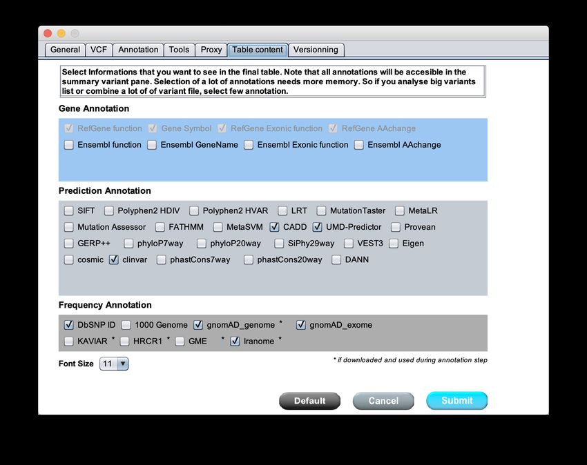
113.5 Table content
Figure 7: Settings panel to configure VarAFT : Result final table content
This section allows the selection of informations to include in the final result table. This part
does not correspond to the settings of annotation process, but rather to which information you
would like to see within the variant result table. Even if not selected, all these informations will
always be available in the variant panel associated with the result table (shown in 39). Please note
that, more columns you add, more memory will be required for the application to run.
The available annotations are detailed below:
Gene Annotation
The RefGene information is mandatory. To perform filter on Ensembl model you must select
associated informations.
• (REQUIRED) RefGene Function: localization of the variation (exonic, splicing, in-
tronic, UTR, ...)
• (REQUIRED)Gene Symbol: official gene symbol
12• (REQUIRED)RefGene Exonic Function: impact of the variation (synonymous, non-
synonymous, stop, frame shift, non frameshift ...)
• (REQUIRED)RefGene AAChange: impact of the variation on each transcripts and
proteins according to the HGVS nomenclature (c. and p.)
• Ensembl Function: localization of the variation (exonic, splicing, intronic, UTR, ...) based
on Ensembl data
• Ensembl Genename:: Ensembl unique gene id (ENSG00000XXXXX)
• Ensembl Exonic Function: impact of the variation (synonymous, non-synonymous, stop,
frame shift, non frame shift ...) based on Ensembl data
• Ensembl AAChange: impact of the variation on the transcripts and proteins according to
the HGVS nomenclature (c. and p.) based on Ensembl data
Prediction Annotation
• SIFT: SIFT pathogenicity prediction.
• PolyPhen2 HDIV: Polyphen2 pathogenicity predictions based on the HDIV dataset.
• PolyPhen2 HVAR: PolyPhen2 pathogenicity predictions based on the HVAR dataset.
• LRT: Predictions from LRT.
• MutationTaster: Predictions from MutationTaster.
• MetaLR: Predictions from MetaLR system.
• Mutation Assessor: Predictions from Mutation Assessor.
• FATHMM: Predictions from FATHMM tool.
• MetaSVM: Predictions from MetaSVM.
• CADD: Phred scores from CADD.
• UMD-Predictor: Predictions from UMD Predictor tool
• Provean: Predictions based on Provean tool.
• GERP++: Prediction scores from GERP++ tool.
• PhyloP7way: PhyloP scores based on multiple alignments of 7 genomes. The larger the
score, the more conserved is the site.
• PhyloP20way: PhyloP scores based on multiple alignments of 20 genomes. The larger the
score, the more conserved is the site.
• SiPhy29way: SiPhy scores based on multiple alignments of 29 genomes. The larger the
score, the more conserved is the site.
13• VEST3: Prediction scores based on VEST3 tool.
• cosmic70: Data from the COSMIC database.
• clinvar: Data from ClinVar database.
• phastCons7way: phastCons scores based on multiple alignments of 7 genomes. The larger
the score, the more conserved is the site.
• phastCons20way: phastCons scores based on multiple alignments of 20 genomes. The
larger the score, the more conserved is the site.
• DANN: Prediction scores from the DANN tool.
Frequency Annotation
• DbSNP ID: rsID of dbsnp from selected version
• 1000 Genomes: Observation frequencies from the 1000 Genomes project version of October
2014 with all ethnicities.
• gnomAD XXX: Frequence of observation for the Genome Aggregation Consortium. Fre-
quence are provided for genome or exome.
• KAVIAR: Variant frequencies from the Known Variant Project (170 Million variants).
• HRCR1: Variant observation frequencies from the Haplotype Reference Consortium (40
Million variants).
• GME: Variant observation frequencies from the Great Middle East database.
• Iranome: Variant observation frequencies from the Iranome database.
Frequency Annotation
Change font size for the table which contains results
3.6 Versionning
This section displays all version of software and annotation data used by VarAFT for the current
version. Informations for previous versions are available in the "Version History" section of the
documentation.
14Figure 8: Settings Panel to configure VarAFT : Versionning
154 Annotation Tool
Figure 9: Menu Annotation Tool
The first step to analyze a variants file is to annotate all variations. In order to accomplish this,
VarAFT implements ANNOVAR, a command line tool. In the Annotation Tool Menu you have
3 options :
• 1 Variant Files Annotation: Module for annotation of a variants file as VCF file.
• 2 UMD-Predictor: Module to retrieve prediction scores from UMD-Predictor. These score
are automatically retrieved during annotation process. However you could need to get it
separately.
• 3 Manage Annovar Database: With this module you can download the needed databases
for the annotation process.
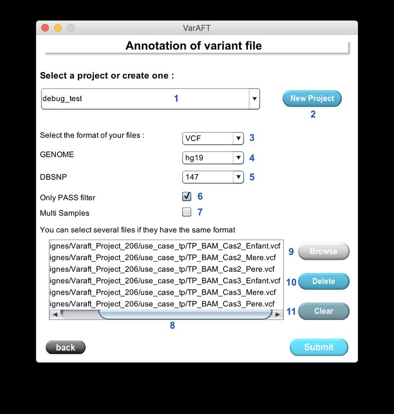
164.1 Variant Files Annotation
Figure 10: Annotation panel to configure and launch the annotation process.
To annotate variants you must first select a specific project (Figure 10: 1). If the project has not
been created yet, a new project will be created by clicking New Project (Figure 10: 2). A new
directory is created in the Varaft_Project folder, defined in the settings.
The second step is the selection of the file format (Figure 10: 3). There are 3 formats available:
VCF, GVCF, ANN, VCF (CNV).
• VCF (Variant Call File) is the standard format used to list all variants into a file. Depending
on the variant caller, the vcf may be not recognized or incorrectly annotated. If this occurs,
please contact us with an example file. We will do our best to solve this issue. However
most VCF files should be properly defined and annotated with VarAFT. Since version 2.13
VarAFT accepts gzip file.
17Figure 11: Variant Call Format example
18• gVCF (Genomic Variant Calling Format). A gVCF is a kind of VCF, so the basic format
specifications are the same as for a regular VCF, but a genomic VCF contains extra infor-
mation such as sequenced regions that are identical to the reference genome. Since version
2.13 VarAFT accepts gzipped VCF file.
• ANN is a basic format. If you don’t have a VCF file you can create your file in an ANN
format. This file is a tab delimited file with 9 columns : Chromosome, Position start, Posi-
tion end, Reference Allele, Alternative Allele, Genotype (SNV/INDEL = het or hom; CNV
= DEL-HTZ; DEL-HOM or DUP), Depth ( Size for CNV) ,Frequency of alternatice allele
(Copy Number for CNV) and score for alternative allele.
You can see an example below :
chr1 955597 955597 G T het 31 0.55 64.48
chr1 977031 977031 G A het 43 0.42 47.28
chr1 977330 977030 T C het 161 0.52 261.78
chr1 980824 980824 G C het 83 0.39 68.26
chr1 10408838 10408838 T - hom 96 0.98 459.98
chr2 32361482 32361482 - C het 9 0.71 -1
Table 1: ANN file format with SNV/INDEL data
chr1 955597 955597 0 - DEL-HTZ 90007 1 100
chr1 977031 977031 0 0 DUP 48521 6 150
chr1 977330 977030 0 - DEL-HTZ 1 0.52 210
chr1 980824 980824 0 - DEL-HOM 0 0.39 170
chr1 10408838 10408838 0 0 DUP 114029 3 120
chr2 32361482 32361482 0 - DEL-HTZ 13885 1 50
Table 2: ANN file format with CNV data
In a third step, it is required to select the genome version (Figure 10: 4). Currently, two versions
are available on VarAFT : HG19 and HG38. For both versions, databases should be downloaded
before use.
The fourth step consists in the selection of dbsnp version (Figure 10: 5). By default, only the
version 147 is downloaded. If you need to use another version of dbsnp go to the Download DBSNP
module (4.4.1).
In the next step you can choose which variants to annotate. The Only PASS filter allows
the annotation of only variants which have passed the variant calling filter criteria (filter flag =
PASS). If you uncheck this option all variants will be annotated.
19WARNING
No all VCF files have the flag filter description (PASS or other). Please check your VCF
before. Annotation of a VCF with no PASS flag but with this option selected will result
into an empty file and no variants will be annotated.
The Multi Samples option (Figure 10: 6) allows to specify if your VCF file contains several
samples into one file. If you annotate a multi sample VCF without check-in this box, only the first
sample will be considered.
Once all options are set, select one or several files that you want to annotate with the Browse
button (Figure 10: 9). You could select several file. All selected files will be displayed in the list
box (Figure 10: 8). To remove one file click on Delete (Figure 10: 10). To remove all files from
the list click on Clear (Figure 10: 11) .
To launch the annotation click on the submit button. A progress bars shows you the progression
of the annotation process. Depending on the file size and your hardware computer, the processing
time will differ.
NOTE
With 4 threads and a VCF with 100000 variants, the process should take between 5 to 15
minutes depending of the optional database selected.
WARNING
For whole genome or whole exome with more intronic region, the HSF annotation could
take a long time. HSF needs to compute all variants that could affect splicing some of those
may take some time to be processed. Note If you reannote the same VCF file the HSF
annotation will be quicker.
4.2 UMD-Predictor
UMD-Predictor allows you to retrieve pathogenicity prediction scores from UMD-Predictor. (see
3.4.1) .
20Figure 12: UMD-Predictor Module
To annotate specifically an annotated file with UMD-Predictor pathogenicity prediction scores,
you have first to select a project (Figure 12: 1) with previously annotated files. To select files click
on Browse (Figure 12: 3). To remove one file click on Delete (Figure 12: 4). To remove all files
from the list click on Clear (Figure 12: 5) .
To launch the annotation process click on the submit button. A new window displays the
progression of the process.
WARNING
Depending on your network configuration, the UMD-Predictor’s webservice may not be
accessible. Contact you administrator network to allow connection to umd-predictor.eu.
4.3 Human Splicing Finder
Human Splicing Finder (HSF) allows you to retrieve prediction from the API of HSF. (see 3.4.2) .
21Figure 13: HSF Module
To retrieve HSF predictions from a previously annotated file, you have first to select a project
(Figure 13: 1). To select files click on Browse (Figure 12: 3). To remove one file click on Delete
(Figure 13: 4). To remove all files from the list click on Clear (Figure 12: 5) .
To launch the annotation process, click on the submit button. A new window displays the
progression of the process.
NOTE
HSF predictions were retrieved during the annotation process, this module allows to rean-
note a previously annotated file if an error occurs during the HSF process. This module
also allows to annotate file coming from VarAFT 2.10 when HSF API annotations were not
available yet.
224.4 Manage Database
Figure 14: Manage Database Module
To perform variant annotation, you have to download various files that will serve as database. If
you want to download data for the Human Genome version 19 click on Download data for hg19.
If you want to download data for the Human Genome version 38 click on Download data for
hg38. These two modules automatically launch the download process et unzip downloaded files in
the database directory specified in Settings (3.1). The download process takes long time (1 hours
to several hours according to your network) and requires various between 30 and 50 GB free space
on your storage support. If you computer/server has several hard drive, it is advice to store the
database on a different disk than the VarAFT_Project folder.
234.4.1 Download dbSNP
The main goal of this Download dbSNP module is to automatically download a specific version
of dnSNP (if the dbSNP version downloaded with the Download data for hg19 or 38 does not
respond to your needs). Indeed only the dbsnp version 150 was downloaded from the two previous
modules.
Figure 15: dbSNP download module
To download an other version of dbSNP, select the genome version (Figure 15: 1) and the
dbSNP version (Figure 15: 2). Some versions exists in a flagged version (that means: no clinical
flagged variant and no variant with MAF lower than 1% ). To select the flagged version check the
box (Figure 15: 3). The following table shows you which version are available:
24Genome Version dbSNP version Flagged version available
HG19 130 Yes
HG19 131 Yes
HG19 132 Yes
HG19 135 Yes
HG19 137 Yes
HG19 138 Yes
HG19 144 No
HG19 147 No
HG19 150 No
HG38 144 No
HG38 147 No
HG38 150 No
Table 3: Available DBSNP version
254.4.2 Create DBLocal
Figure 16: Module for creation of local database
Sometimes you might need to filter out your variants with specific personal data such as specific
ethnic variants or known artifacts.
The aim of this module is to easily create a such file with all your variants and use it as a filter
option in your variant filtration analysis.
To build this file, first provide a name (Figure 16: 1). Next select the format of the input files
(VCF or ANN 4.1 ) (Figure 16:2). Choose to use this file by default (Figure 16: 3). In the next
step you can decide if you want to keep variants that were able to pass quality filters or not. To
do so check or uncheck the Only PASS filter. If you uncheck this option all variants will be
considered (Figure 16:4).
To select files click on Browse (Figure 16: 5). To remove one file click on Delete (Figure 16:
6). To remove all files from the list click on Clear (Figure 16: 7) . If a VCF file contains several
samples, each samples will be considered. Since VarAFT 2.13 gzip VCF are accepted.
26The output file look like as follow :
mutation_id chromosome position reference observed nb_ind_nb nb_ind_hom nb_ind_all nd_ind_total
1 chr1 879676 G A 0 1 1 290
2 chr1 879687 GC G 3 0 3 290
4 chr1 881627 T TCTC 1 0 1 290
7 chr1 888639 TTC T 0 5 5 290
Table 4: Example local database
275 Analysis and filter tool
Figure 17: Analysis and filter tool module: Method selection
285.1 Manual Filtering
Figure 18: Analysis and filter tool module: Project selection
This module allows you to combine and filter your annotated variant files. Several features are
available. To start an analysis, select a project and click next (Figure 18).
29Figure 19: Main panel of VarAFT for analysis
The main panel of VarAFT is composed of 4 parts ( Figure 19 ):
• Area 1: Selection of combination mode. It is possible to combine data from multiple
samples/patients (singleton, trio or any combination)
– Autosomal Recessive Disease
∗ Index Case only
∗ Trio Analysis both Parents/Proband
∗ Multi Analysis (vcf merged)
– Autosomal Dominant Disease
∗ Index only
∗ Trio Analysis with both Parents/Proband (for de novo analysis)
– Custom analysis
∗ Cohort analysis at:
· the variation level (variants shared by several individuals).
· the gene level (Genes with variation shared by several individuals.)
30∗ Somatic variation identification by comparing Normal vs Tumoral sample.
∗ any other type of combination between individuals
• Area 2: Results table. This area displays the list of selected variations with main an-
notations. A click on a row will update area #4. A right click on a row gives access to a
contextual menu which allows to :
– access IGV and visualize read alignment data
– show tissues expressions
– get data from HSF - Human Splicing Finder
– access several links (NCBI, UCSC, OMIM, GeneCards . . . )
• Area 3: Filtration Area. This area allows you to define and apply filtration criteria such
as :
– Variation type and localization
– Frequency
– Pathogenicity predictions
– Genes information
– Others (Clinvar, Cosmic ...)
• Area 4: Information Area. This area provides detailed information on the selected variant:
– Nomenclature in all transcripts
– Variants Information for each samples
– Frequency in the general population
– Pathogenicity Predictions
– Localization in particular regions
– Pathways (KEGG, REACTOME, PID)
– Gene Ontology
– OMIM
– Tissues Expression from GTEX
– External links
5.1.1 Mode of inheritance
5.1.1.1 Autosomal Recessive Disease Six kinds of analysis are available: Index Case Anal-
ysis, Trio Analysis and Multi Analysis. Output results depend on different possible cases (Figure
20).
31Figure 20: Autosomal Recessive Disease Schema
Index Case Analysis To perform the analysis of a index case click on .
A new panel appears (Figure 21). Click on the browse button (Figure 21: 2) to select the
annotated file corresponding to the index case. To keep uncertain heterozygous variants (more
information in section 3.3) let the box checked (Figure 21: 3) if not uncheck it.
To select of a gene list check the box ((Figure 21: 4). To add a new gene list show section 7.1.
You can use a BED file to filter your data, for that check the box ((Figure 21: 5).
To launch the analysis click on the submit button. A progress bar shows you the progression of
the process.
Once the analysis is completed, 3 tabs will appear: one for homozygous hypothesis, one for com-
pound heterozygous hypothesis, and one with heterozygous one (only gene with one variant).
Trio Analysis To perform a trio family analysis, click on .
A new window appears (Figure 22). Click on the browse buttons to select the following files: the
annotated file corresponding to the proband (Figure 22: 1), the annotated file corresponding to
32Figure 21: Index analysis configuration panel
the Mother (Figure 22: 2) and the annotated file corresponding to the Father (Figure 22: 3).
To keep uncertain heterozygous variants (more information in section 3.3) let the box checked
(Figure 22: 4) if not uncheck it.
To select of a gene list check the box ((Figure 22: 5). To add a new gene list show section 7.1.
You can use a BED file to filter your data, for that check the box ((Figure 22: 6).
Once all files have been selected, click on the submit button to continue.
Once the analysis completed, 6 results tabs will appear:
• Homozygous variations (the same variation : 1 heterozygous from father, 1 heterozygous
from mother )
• Compound heterozygous (2 variations : 1 heterozygous from father, 1 heterozygous from
mother )
• Homozygous with only Father Heterozygous for the same variation
• Homozygous with only Mother Heterozygous for the same variation
• Heterozygous with Father Heterozygous for the same variation
33Figure 22: Autosomal Recessive Disease : Trio Analysis
• Heterozygous with Mother Heterozygous for the same variation
Family Analysis To perform the analysis of a family based on a multi annotated VCF file
click on .
34Figure 23: Autosomal Recessive Disease : Family Analysis 1/2
A new window appears (Figure 23). Click on the browse button to select the file (Figure 23: 1).
To keep uncertain heterozygous variants (more information in section 3.3) let the box checked
(Figure 23: 2) if not uncheck it.
To select of a gene list check the box ((Figure 23: 5). To add a new gene list show section 7.1.
You can use a BED file to filter your data, for that check the box ((Figure 23: 6).
Once all files have been selected, click on the submit button to continue.
35Figure 24: Autosomal Recessive Disease : Family Analysis 2/2
In the next window (Figure 24), set the status for each sample. Each row correspond to one
sample. For one row click on the Sample column to choose the status of the sample. You have
the choice between 6 options :
• Affected: set if the sample is affected.
• Mother: set if the sample is the mother
• Father: set if the sample is the father
• Healthy: set if the sample is healthy
• Healthy Carrier: set if the sample is healthy carrier.
• No: set if you don’t want to use this sample in your analysis.
You have to define at least a Mother and a Father, these are mandatory.
Once the analysis is completed, 6 results tabs will appear:
• Homozygous variations (the same variation: 1 heterozygous from father, 1 heterozygous from
mother )
• Compound heterozygous (2 variations: 1 heterozygous from father, 1 heterozygous from
mother )
• Homozygous with only Father Heterozygous for the same variation
• Homozygous with only Mother Heterozygous for the same variation
36• Heterozygous with Father Heterozygous for the same variation
• Heterozygous with Mother Heterozygous for the same variation
375.1.1.2 Autosomal de novo Dominant Disease Two kinds of analysis are available: Index
Case Analysis, Trio Analysis (de novo).
Index Case Analysis To perform the analysis of an index case click on .
Figure 25: Index analysis configuration panel for Autosomal dominant disease
A new panel appears (Figure 25). Click on the "browse button" (Figure 25: 1) to select the
annotated file corresponding to the index case. To keep uncertain heterozygous variants (more
information in section 3.3) let the box checked (Figure 25: 2) if not uncheck it.
The last option allows you to add a selection of genes (gene list). For that check the box ((Figure
25: 3) and select your list. To add a new gene list show section 7.1.
You can use a BED file to filter your data, for that check the box ((Figure 25: 4).
Once all files have been selected, click on the submit button to continue.
Once the analysis is completed, 1 tab will appear with all heterozygous variant.
38Trio Analysis To perform the analysis of a trio family click on .
Figure 26: Autosomal Recessive Disease : Trio Analysis
A new window appears (Figure 26). Click on the browse buttons to select the following files:
the annotated file corresponding to the proband (Figure 26: 1), the annotated file corresponding
to the Mother (Figure 26: 2) and the annotated file corresponding to the Father (Figure 26: 3).
To keep uncertain heterozygous variants (more information in section 3.3) let the box checked
(Figure 26: 4) if not, uncheck it.
The last option allows you to add a selection of genes (gene list). For that check the box
((Figure 26: 5)) and select your list. To add a new gene list show section 7.1.
You can use a BED file to filter your data, for that check the box ((Figure 26: 6).
Once all files have been selected, click on the submit button to continue.
Once the analysis completed, 1 tab will appear with proband specific heterozygous variant (Not
present on both parents) .
395.1.1.3 Custom Analysis To perform a custom analysis click on .
Figure 27: Custom Analysis Module
A new window appears (Figure 27). Click on the browse button (Figure 27: 1) to select all
wanted files. Single or multi files are allowed. Annotated files with CNV can be combined with
SNV/INDELs annotated files. If you want to select a genes list, check the box (Figure 27: 4) and
select your list. To add a new gene list show section 7.1.
You can use a BED file to filter your data, for that check the box ((Figure 26: 6).
To continue click on submit.
40Figure 28: Custom Analysis Module Configuration
You get a new window with all selected samples in a table. You can choose between the two
following options:
• Get variants from each sample with selected genotype (Figure 28: 1): With this
option all the genotypes given in part 5 will be considered.
• Get variants with minimal number of conditions and selected genotype (Figure
28: 2): the genotype can be chosen for all files. After choosing this option, whether you want
"Variants" or "Genes" (Figure 28: 3) and the threshold (Figure 28: 4) must be chosen.
For example, you have 4 files for which you select the genotype Heterozygous. If you select
"Variant" and a threshold of 3/4 that means you want all the variants to be present in 3
out of the 4 files given with the selected genotype. If you select "Gene" and a threshold of
3/4 that means you want all genes present in 3 files out of the 4 given whatever the variant.
Next you must set the genotype for each sample. Each row correspond to one sample.
41For one row, click on the Genotype column (Figure 28: 7) to choose the genotype of the sample.
You have the choice between 5 options for SNV/INDELs data :
• ALL: all variations, whatever the genotype
• HTZ: Heterozygous variations
• HOM: Heterozygous variations
• ABS: the variation must be absent. (this option is not available for "Select minimal number
of conditions")
• ND: the variation may be present or absent depending on the genotype. (this option is not
available for "Select minimal number of conditions")
• NO: Not used the corresponding sample. Very useful to analyze some samples from merges
VCF.
You have the choice between 4 options for SNV/INDELs data :
• ALL: all variations, whatever the genotype
• DEL-HTZ: CNV Heterozygous deletion
• DEL-HOM: Heterozygous deletion
• DUP: CNV duplication
You can set several rows in one time. For that select rows and click on the right button of your
mouse and select between :
• Set All
• Set Homozygous
• Set Heterozygous
• Set Absent (this option is not available for "Select minimal number of conditions")
• Set Not Defined (this option is not available for "Select minimal number of conditions")
Once you have selected your settings you can click on submit. Once the analysis completed,
one result tab will appear with variations corresponding to the parameters previously selected.
425.1.2 Filtration area
Figure 29: Filtration Area
The filtration area is divided in 5 tabs (Figure 29):
• Variant Type
• Frequency
• Prediction
• Genes Information
• Others
On the right you can see 6 buttons (Figure 29):
• 1: Show/hide the filter area.
• 2: Apply saved filters for the selected project.
• 3: Save filters for the the selected project.
• 4: Apply default filters
• 5: Save filters as default (available for all projects)
• 6: Reset filters
435.1.2.1 Variant Type From the first tab (Figure 29) you can filter variants based on the type
and/or the functional effect. To filter a specific item, uncheck the associated box. By right clicking
you can select or unselect all items.
NOTE
Since VarAFT 2.13 you can choose between RefSeq or Ensembl gene models. To use En-
sembl source, select associated columns in the setting (cf. 3.5)
Figure 30: Filter based on the population frequency data. Annotation with version < 2.10
44Figure 31: Filter based on the population frequency data. Annotation with version >= 2.10 and
< 2.16
45Figure 32: Filter based on the population frequency data. Annotation with version >= 2.16
5.1.2.2 Frequency
Public database The second tab allows you to filter variants based on the population fre-
quency. Several public databases are currently available in the new version.
• 1000G: Data from 1000 genomes project (08-2015).
• gnomAD: Data from Genome Aggregation Consortium version 2.11 (since 2.16). 7 subpop-
ulation and 8 subgroups are available. gnomAD Exome is always used. gnomAD Genome is
optional and must be selected in the settings to be used.
– AMR: Latino population
– AFR: African population
– SAS: South Asian population
– EAS: East Asian population
– NFE: Non Finnish European population
– FIN: Finnish European population
– ASJ: Ashkenazi Jewish Population
– OTH: Others population.
– RAW: Allele Frequency from Raw data(since 2.16)
46– MALE: Allele Frequency for Male only (since 2.16)
– FEMALE: Allele Frequency for Female only (since 2.16)
– MAX: This annotation contains a threshold filter allele frequency for a variant. Tech-
nically, this is the highest disease-specific maximum credible population AF for which
the observed AC is not compatible with pathogenicity. See gnomAD documentation for
more details (since 2.16)
– NON TOPMED: Only samples that are not present in the Trans-Omics for Precision
Medicine (TOPMed)/BRAVO release. The allele counts in this subset can thus be
added to those of BRAVO to federate both datasets. (since 2.16)
– NON NEURO: Allele Frequency with Only samples from individuals who were not
ascertained for having a neurological condition in a neurological case/control study
(since 2.16)
– NON CANCER : Only samples from individuals who were not ascertained for having
cancer in a cancer study (since 2.16)
– CONTROLS: Only samples from individuals who were not selected as a case in a
case/control study of common disease (since 2.16)
• KaViar: Data from Known VARiants Project. Kaviar contains 162 million SNV sites (in-
cluding 25M not in dbSNP) and incorporates data from 35 projects encompassing 77,781
individuals (13.2K whole genome, 64.6K exome). This database is optional and must be
selected in the settings to be used.
• HRC: The Haplotype Reference Consortium. This database is optional and must be selected
in the settings to be used.
• GME: The Great Middle East database. This database is optional and must be selected in
the settings to be used.
• Iranome: The Iranome database. This database is optional and must be selected in the
settings to be used (since 2.16).
You can also remove all variants with a dbsnp id by clicking on Remove DBSNP.
Warnings : By default DbSNP database contains data from clinical source and variants with a
allele frequency above 1%. Be careful using this option.
Local database Thanks to VarAFT you have the possibility to generate a local database
with a selection of VCF files (show 4.4.2). If you have set a default dblocal file you can filter
your variants list thanks to this database. The value Max will be automatically update with your
dblocal. You can select between ALL, HET (Heterozygous) and HOM (Homozygous) and set the
minimal threshold to perform the filter.
The button Filter based on File of variant offers two options (Figure 33) : show or filter
variants. Two format file are available: a text file as dblocal (show 4) or a bed file. The bed file
must have the following format :
47chr1 879676 879677 Variant1
chr1 879687 879689 Variant2
chr1 881627 881628 Variant3
chr1 888639 888642 Variant4
Table 5: Example bedfile
Figure 33: Filter based on a file of variant
48Figure 34: Filter based on prediction score.
5.1.2.3 Prediction The third tab allows you to select variants based on the prediction scores.
Several different tools are available: UMD-Predictor, Human Splicing Finder, SIFT, PolyPhen, Mu-
tation Taster, Mutation Assessor, Provean, LRT, M-CAP, Eigen, DANN, CADD and GERP++.
For the first height tools, simply uncheck the boxes of the non-desired prediction. For DANN,
Eigen, CADD and GERP++, no classification exists, so a cut-off needs be selected to apply a
selection.
49Figure 35: Filter based on gene informations.
5.1.2.4 Gene Informations The fourth tab allow for filtration thanks to informations relative
to genes. Several options are available.
Gene Name Select all variants localized in a specific gene by providing a gene name. It is a
case sensitive research.
Score Different scores gene specific are available:
• RVIS: RVIS score measures genetic intolerance of genes to functional mutations, as described
in Petrovski et al. Original RVIS was constructed based on patterns of standing variation
in 6503 samples. The authors have recently constructed scores based on the 61,000 samples
from ExAC. There is high correlation, but more resolution for many genes. A gene with a
positive score has more common functional variation, and a gene with a negative score has
less and is referred to as "intolerant".
• GDI: the gene damage index (GDI) represents the accumulated mutational damage for
each human gene in the general population, and shows that highly mutated/damaged genes
are unlikely to be disease-causing and yet they generate a big proportion of false positive
variants harbored in such genes. Therefore removing high GDI genes is a very effective way
to remove confidently false positives from WES/WGS data. The data set includes general
damage prediction (low/medium/high) for different disease type (all, Mendelian, cancer, and
PID).
50• LoFTool: gene loss-of-function score percentiles. The smaller the percentile, the most in-
tolerant is the gene to functional variation.
• GHIS: Genome-wide HaploInsufficiency Score. Higher is the score, the most haploinsuffi-
ciency is the gene.
Pathway & GO & HPO & OMIM Different database are available to filter variants.
• KEGG: KEGG is a database resource for understanding high-level functions and utilities of
the biological system, such as the cell, the organism and the ecosystem, from molecular-level
information, especially large-scale molecular datasets generated by genome sequencing and
other high-throughput experimental technologies.
• REACTOME: Reactome is a free, open-source, curated and peer reviewed pathway database.
The goal is to provide intuitive bioinformatics tools for the visualization, interpretation and
analysis of pathway knowledge to support basic research, genome analysis, modeling, systems
biology and education.
• PID: The Pathway Interaction Database (PID, http://pid.nci.nih.gov) is a freely available
collection of curated and peer-reviewed pathways composed of human molecular signaling
and regulatory events and key cellular processes.
• GO: Gene Ontology is the framework for the model of biology. The GO defines concepts/-
classes used to describe gene function, and relationships between these concepts. It classifies
functions along three aspects: molecular function(molecular activities of gene products), cel-
lular component (where gene products are active) and biological process (pathways and larger
processes made up of the activities of multiple gene products).
• HPO: The Human Phenotype Ontology (HPO) aims to provide a standardized vocabulary
of phenotypic abnormalities encountered in human disease. Each term in the HPO describes
a phenotypic abnormality, such as atrial septal defect.
• OMIM: OMIM is a comprehensive, authoritative compendium of human genes and genetic
phenotypes that is freely available and updated daily. The full-text, referenced overviews in
OMIM contain information on all known mendelian disorders and over 15,000 genes. OMIM
focuses on the relationship between phenotype and genotype. It is updated daily, and the
entries contain copious links to other genetics resources.
51Figure 36: Pathways filtering module
The version 2.10 introduce a new module to combine data from KEGG, REACTOME, PID,
OMIM, HPO and GO. This module allows to retrieve list of genes from selected annotation.
To do that, first select the database (Figure 36: 6) click on the desired item(s) in the list (Figure
36: 9). This list is populated with the gene list from the result table (after applied filters). If you
want to get genes from this list click on the ’»’ button (Figure 36: 7). The selected items are added
in the box (Figure 36: 3) and the associated genes are added in the box (Figure 36: 5). If you
want excluded genes from the final list, select item and click on "»" button (Figure 36: 8). The
selected items are added in the box (Figure 36: 4) and the associated genes are removed from the
box (Figure 36: 5). You can save the obtained genes list thanks to the button (Figure 36: 1).
52Figure 37: Gene Tissue Expression
GTEx The Genotype-Tissue Expression (GTEx) project aims to provide to the scientific
community a resource to study human gene expression and regulation and its relationship to
genetic variation. This project will collect and analyze multiple human tissues from donors who
are also densely genotyped, to assess genetic variation within their genomes. You can use these
data to select variants in genes expressed in a particular tissue.
The figure 37 shows the panel corresponding to GTEx. First select one or several tissue. Next
select a minimal expression threshold (TPM >2) and last if you have selected more than 1 tissue
set a threshold to choice the minimal number of tissue that it must expressed the gene.
Click on submit. Only variant in genes expressed in the selected tissue are kept.
535.1.3 Others
Figure 38: Other filtering options
• 1. Select by position. You could select variants with only a chromosome or with a specific
position.
• 2. Filter variants based on the SNV score. The SNV score is a Phred quality score given by
the variant caller. Set a threshold and click on the green button.
• 3. Clinvar: you can either keep or remove variants include in Clinvar. You also have the
possibility to select between All, Benign or Pathogenic.
• 4. Cosmic: you can either keep or remove variants include in cosmic (v70).
• 5. Get Compound Heterozygous: In a autosomal recessive disease hypothesis you want
to keep only gene with at least 2 variants. Once you performed several filtering steps, several
genes are not compliant with this hypothesis. To solve this issue click on the button Get
Compound Heterozygous. Click on the circle arrow to reset this filter.
• 6. Get Genes with threshold: In a cohort analysis with the custom mode, you have
the possibility to select genes shared by several sample according to a threshold. Once you
performed several filtering steps, several genes are not compliant with this hypothesis. To
solve this issue click on the button Get Genes with threshold. Click on the circle arrow to
reset this filter.
545.1.4 Variant Informations
Figure 39: Panel containing variant information 1/3
55Figure 40: Panel containing variant information 2/3
56Figure 41: Panel containing variant information 3/3
This area provides detailed information on the selected variant (Figure 39, 40 & 41 ):
• General Information: Gene name, position (with genome version), reference allele, alternative
allele and functional impact are displayed.
• RefGene Transcript Information: List of all refseq id with the associated HGVS nomencla-
ture.
• Ensembl Transcript Information: List of all ensembl transcript id with the associated HGVS
nomenclature.
57• Database frequency population: Frequency in several database including ExAC, Exome vari-
ant server, 1000 Genomes, KaViar and HRC.
• Clinvar: List of Clinvar ID with conclusion and link to clinvar website for the variant.
• Cosmic: List of Cosmic ID with link to cosmic website for the variant.
• Prediction Tools: All prediction score for the selected variant.
• Human Splicing Finder: All prediction and interpretation from HSF foreach transcript.
• KEGG : List of KEGG pathway
• Reactome : List of Reactome pathway
• PID : List of PID pathway
• Gene Ontology: list of Gene Ontology
• OMIM : list of OMIM disease with description
• Tissus Expression from GTEX: Histogram of RPKM value for each tissue
• External links : Links to UCSC, GeneCards, NCBI, OMIM, Malacards, GTEx Portal.
585.1.5 Result table
Figure 42: Table with all variants resulting of your analysis and filtering
The result table (Figure 42) contains several fixed columns:
• Chr: Chromosome name
• Start: Start positon of the variant
• End: End position of the variant
• Ref : Reference Allele
• Alt: Alternate Allele
• Genotype *: Genotype
• Depth *: Number of used reads at the position of the variant
• Frequency *: Number of reads containing the alternate allele divided by the depth.
• SNV Score *: quality score of the variant given by the variant caller.
• Func.refgene: localisation of the variation (exonic, splicing, intronic, UTR, ...)
• Gene.refgene: Gene Symbol
• ExonicFunction.refgene: impact of the variation (synonymous, non-synonymous, stop,
frameshift, non frameshift ...)
• AAChange.refgene: detailed variation on the transcript and on the protein (c. and p.)
• Var in File (only available with the option "Select minimal number of conditions"): Number
of files containing the variation on the total of files.
• Gene in File (only available with the option "Select minimal number of conditions" and
"Gene"): Number of files containing the gene on the total of files.
• *: Only if one sample is analyzing or if you use Trio analysis.
59The table also contains annotations that have been selected in Settings (3.5).
A popup menu appears by clicking right button of your mouse on a row. In this popup menu
you access to:
• Remove Line(s): Remove the selected row(s).
• Show on IGV: Display selected bam files at the variant position on the Interactive Genome
Browser.
• Gene Expression: show the histogram with expression level of the selected gene for each
tissue.
• Links: Links to Malacards, GeneCards,OMIM,UCSC,NCBI,GTEx Portal.
5.1.6 Other Options
Figure 43: Other options
At the bottom of the main window, you can see the number of variants (Figure 43 1), the number
of genes (Figure 43 2) and the project name (Figure 43 3). You have 5 buttons :
• 4: Display selected bam files at the variant position on the Interactive Genome Browser.
• 5: Save results table in VarAFT format. The output file could be reopen in custom mode
and / or combine with other result or samples.
• 6: Save results table in excel format. The file contains a header with information about
analysis as the used samples and the used filters.
• 7: Print results table.
• 8: Display information about analysis.
605.2 Automatic Filtering VarAFT introduces a new filter mode in the version 2.10. It is the automatic filtering module. This module allows to pre-filter several annotated files. For example it was very useful to prefilter big annotated files from whole genome. It can reduce the number of variants by 10,000 only with simple filter options. The process is very easy and quick. Just choose your files, select the filter criteria and apply. INFORMATION A annotated files of 4,781,755 variants was reduced to 178 variants in 30 seconds with filters based on the variant type (exonic), frequencies (
To use this module, first set the filter options (Figure 44 1): As in the manual mode you have
access to several options:

   • Variant type and variant impact (Figure 45 ): Uncheck the box of items that you want
     remove from your files.
   • Public Database (Figure 46 ). Select the database that you want to use and set the
     threshold. "
Figure 46: Auto filtering : Public database
Next select the annotated files (Figure 44.8) and submit.
A new windows show you the progression.
63Figure 47: Auto filtering : Pathogenicity Prediction
646 Coverage Analysis
The last main module of VarAFT allow for computation of coverage from BAM files.
Figure 48: Coverage Menu Panel
From the menu you have 3 options (Figure 48):
• Compute Coverage: Module to compute the coverage from one or several BAM files.
• Show Coverage: Module to show output of the coverage analysis with interactive charts.
• Create BED: Module to create un bed file (with coding exon) from a gene list.
656.1 Compute Coverage
Figure 49: Module to compute coverage from BAM files
To perform the coverage analysis, first select a project (Figure 49 1) or create a new one (Figure
49 2). Next select the genome version between hg19 (GRCh37) or hg38 (GRCh38). (Figure 49
3). Select the type of data (Figure 49 4). Next select one or several BAM files thanks to the
browse button (Figure 49 5). Before selecting a bam file check if the associated BAI file is present
in the same folder. Once BAM files are selected, choice between coding-exon, all-exon or custom
mode (Figure 49 8). For coding-exon mode consider only the coding exon of the transcript will
be considered for the coverage analysis. For all-exon mode all the exons of the transcripst will
be considered for the coverage analysis. In custom mode, you must provide a bed file. Here you
can compute coverage for all you want. Select if you want to include the flanking region of exon
(+/- 50 bp) (Figure 49 9). The last step is the selection of a bed file. In coding-exon mode if you
don’t select a bed file all transcripts will be considered. To analyze a panel of genes check the box
(Figure 49 10) and select the bed file in the list. In coding-exon mode the bed file must have a
specific format. You should generate it with the Create Bed module (6.3). In custom mode the
bed file must be selected.
Click on submit button to launch the analysis. Two progress bars show you the advancement
of the analysis.
66WARNING
The GRCh3X versions of the genome don’t contain "chr" in the chromosome name
whereas HGXX versions contain it. Check the version used and generate the appropriate
bed file. If the BAM and BED files are not compliant you will get an error message.
676.2 Show Coverage
To show the coverage analysis results, select Show Coverage and select the project.
Figure 50: Show Coverage Analysis Module
In the new window select the sample in the list and click on "LOAD" (Figure 50 1). A new
tab will be generated containing a table (Figure 50 2). In coding-exon mode each line in the table
corresponds to a transcript. This table contains the following columns:
• RefSeqName: The RefseqMrna ID used to compute the coverage.
• GeneSymbol: The associated GeneSymbol.
• Exon Number: The total number of coding exon in the transcript.
• Size Coding Exons: The size of the coding part of the transcript.
• Mean Depth: The mean depth for the transcript.
• SD Depth: the standard deviation of the depth for the transcript.
68• Coverage 1x: Coverage of transcript at 1x of depth. This means the percentage of bases
read at 1x for the entire transcript (only coding exon).
• Coverage 5x: Coverage of transcript at 5x of depth. This means the percentage of bases
read at 5x for the entire transcript (only coding exon).
• Coverage 10x: Coverage of transcripts at 10x of depth. his means the percentage of bases
read at 10x for the entire transcript (only coding exon)
• Coverage 20x: Coverage of the transcript at 20x of depth. his means the percentage of
bases read at 20x for the entire transcript (only coding exon)
• Coverage 30x: Coverage of the transcript at 30x of depth. his means the percentage of
bases read at 30x for the entire transcript (only coding exon)
Several filtering options are available. It is possible to filter based on the refseq name (Figure
50 6), the gene symbol (Figure 50 5), and the value (Figure 50 7). The value can be selected
from a list of "Mean Depth", "Coverage 1x", "Coverage 5x", "Coverage 10x", "Coverage 20x", and
"Coverage 30x". The limit can be chosen from the following list: >, = or =90% and < 100%, a red bar
indicates an exon with coverage = at 20x, a yellow bar indicates
a base with a depth >= at 10x and < 20x, a red bar indicates a base with a depth < 10x.
If one of the six first columns is clicked on, the chart in the left panel will correspond to the
mean depth for each exon.
69You can also read