NEURAL BOOTSTRAPPER - OpenReview
←
→
Page content transcription
If your browser does not render page correctly, please read the page content below
Under review as a conference paper at ICLR 2021

N EURAL B OOTSTRAPPER
 Anonymous authors
 Paper under double-blind review

                                            A BSTRACT

         Bootstrapping has been a primary tool for uncertainty quantification, and their theo-
         retical and computational properties have been investigated in the field of statistics
         and machine learning. However, due to its nature of repetitive computations, the
         computational burden required to implement bootstrap procedures for the neural
         network is painfully heavy, and this fact seriously hurdles the practical use of these
         procedures on the uncertainty estimation of modern deep learning. To overcome
         the inconvenience, we propose a procedure called Neural Bootstrapper (NeuBoots).
         We reveal that the NeuBoots stably generate valid bootstrap samples that coincide
         with the desired target samples with minimal extra computational cost compared to
         traditional bootstrapping. Consequently, NeuBoots makes it feasible to construct
         bootstrap confidence intervals of outputs of neural networks and quantify their
         predictive uncertainty. We also suggest NeuBoots for deep convolutional neural
         networks to consider its utility in image classification tasks, including calibration,
         detection of out-of-distribution samples, and active learning. Empirical results
         demonstrate that NeuBoots is significantly beneficial for the above purposes.

1    I NTRODUCTION
Since the introduction of the nonparametric bootstrap (Efron, 1979), bootstrap (or bagging) procedures
have been commonly used as a primary tool in quantifying uncertainty lying on statistical inference,
e.g. evaluations of standard errors, confidence intervals, and hypothetical null distribution. This
success is because of its simplicity and theoretical optimality. Under moderate regularity conditions,
the bootstrap procedures asymptotically approximate the sampling variability of statistical procedures,
and its powerful performance in practice was confirmed in various literature (Davison and Hinkley,
1997; Efron, 2000; Hall, 1994). Despite its success in statistics field, the use of bootstrap procedures
in neural network applications has been less highlighted due to its computational intensity. In
uncertainty quantification, bootstrap procedures require evaluating at least hundreds of models, and
this multiple training is infeasible in practice in terms of computational cost.
To utilize bootstrap for deep neural networks, we propose a novel procedure called Neural Boot-
strapper (NeuBoots). The main idea is to construct a generator function that maps bootstrap weights
to bootstrap samples. Our new procedure is motivated from a recent work, Generative Bootstrap
Sampler (GBS) (Shin et al., 2020), in accelerating the computational speed of bootstrap procedure,
but we note that our procedure is strictly different from the GBS. The GBS mainly focuses on classical
models in statistics, and its application is limited to parametric models. In contrast, the NeuBoots is
designed to generate a bootstrap distribution of neural net outputs, and we apply the NeuBoots to
identify uncertainty in prediction via Convolutional Neural Networks (CNNs) (CireşAn et al., 2012;
LeCun et al., 1998). Throughout this paper, we show that our NeuBoots enjoys multiple advantages
over the existing uncertainty quantification procedures.
The NeuBoots is easily applicable to existing various neural networks with a minimal effort. By
constructing a generator function whose input is bootstrap weights, neural networks with the NeuBoots
procedure only require to concatenate bootstrap weights into the input vector of the target network.
This means that the NeuBoots does not inject randomness into the network parameters that are usually
large-numbered, but it directly generates bootstrap samples of the output of the target network. This is
a clear advantage over the Bayesian approaches (Graves, 2011; Louizos and Welling, 2017). Bayesian
Neural Networks (Bayesian NNs) based on variational inference focus on the posterior distribution of
network parameters. However, due to the fact that the number of parameters even in a moderate-sized
network is enormous, evaluating such a high-dimensional distribution is practically challenging in

                                                   1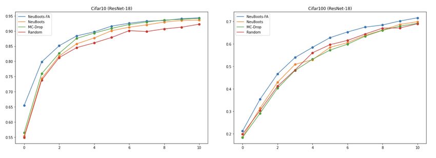
Under review as a conference paper at ICLR 2021

terms of training time and memory resources. In contrast, the randomness of the NeuBoots stems
from the input of bootstrap weights instead of the model parameters. So, the approximation of the
distribution of model parameters, which is high-dimensional, is unnecessary. This property of the
NeuBoots enables us to scalably compute the bootstrap distribution of the output of CNNs such as
ResNet (He et al., 2016) and DenseNet (Huang et al., 2017). These are examined in Section 4.
We theoretically prove that the NeuBoots provides a valid bootstrap distribution of the neural network
of interest. We first show that the vanilla version of the NeuBoots, which constructs the exact bootstrap
distribution, then we adopt the block bootstrap (Carlstein et al., 1998) for scalable approximation
by considering blocks of data observations. Theorem A.2 in the supplementary materials ensures
that this modification is asymptotically equivalent to the conventional non-block bootstrap, and our
empirical results also support this theoretical assertion.
We also apply the NeuBoots to various uncertainty estimation with image classification tasks. First, we
apply our NeuBoots to Out-Of-Distribution (OOD) detection task. We evaluate some scorings from the
bootstrap distribution, including the max of predictive mean, the standard deviation, predictive entropy,
and expected entropy. Then, we train an OOD detector considering the scorings as its input. The
details of the OOD procedure are given in Section 4. Our results show that the NeuBoots outperforms
the state-of-the-art OOD procedures such as ODIN (Liang et al., 2018) and Mahalanobis distance-
based method (Lee et al., 2018). Secondly, we evaluate the confidence estimation performance of
NeuBoots on CIFAR and architectures in Section 4.2. The results show that the proposed methods can
estimate the confidence of the prediction correctly while preserving the classification performance
of the baseline models. Finally, we evaluate NeuBoots on an active learning task, one of the main
application of uncertainty estimation, in Section 4.3. It shows there is a significant performance gap
between the NeuBoots and the other sampling strategies, e.g. MCDrop (Gal and Ghahramani, 2016).

2    R ELATED W ORK

Bootstrapping Neural Network Since Efron (1979) first proposed the nonparametric bootstrap-
ping to quantify uncertainty in general settings, there has been a rich amount of literature that
investigate theoretical advantages of using bootstrap procedures Hall (1986), Hall (1992), and
Efron (1987) showed that bootstrap procedures are capable of achieving second-order correctness.
That means that bootstrapped distribution converges to the target significantly faster than classical
asymptotic approximations that only attain the first-order correctness. Franke and Neumann (2000)
investigated bootstrap consistency of one-layered multi-layer perceptron (MLP) under some strong
regularity conditions. Reed et al. (2014) considered using a conventional nonparametric bootstrapping
to robustify classifiers under noisy labeling. However, due to the nature of repetitive computations,
its practical application to large-sized data sets is not trivial. Nalisnick and Smyth (2017) proposed an
approximation of bootstrapping for neural network by applying amortized variational Bayes. Despite
its computational efficiency, the armortized bootstrap does not induce the exact target bootstrap
distribution, and its theoretical justification is lacking.

Uncertainty Estimation There are many approaches to estimate the confidence intervals of predic-
tion of the deep neural networks. Deep Confidence (Cortés-Ciriano and Bender, 2018) proposes a
framework to compute confidence intervals for individual predictions using snapshot ensembling and
conformal prediction. Also, a calibration procedure to approximate a confidence interval is proposed
based on Bayesain NNs (Kuleshov et al., 2018). However, these approaches do not provide any
theoretical guarantees. In contrast, our theory proves that the NeuBoots generates statistically valid
bootstrap samples. Previously, approximate inference in Bayesian NNs has been proposed mainly
in the literature. Gal and Ghahramani (2016) proposes MCDrop which captures model uncertainty
casting dropout training in neural networks. Smith and Gal (2018) examines various measures of
uncertainty for adversarial example detection. Instead of Bayesian NN, Lakshminarayanan et al.
(2017) proposes a non-Bayesian approach for estimating predictive uncertainty based on ensembles
and adversarial training. Compared to DeepEnsemble, NeuBoots does not require adversarial training
nor learning multiple models, hence its training burden is affordable. Furthermore, NeuBoots does
not suffer performance degradation caused by bootstrap sampling inefficiency. This is because we
use a smoothed version of nonparametric bootstrap called Random Weight Bootstrap (RWB; (Shao
and Tu, 1996)) that utilizes the entire data set unlike nonparametric bootstrap.

                                                   2
Under review as a conference paper at ICLR 2021

3     N EURAL B OOTSTRAPPER
In this section, we first present a reinterpretation of bootstrapping method as a functional on the class
of neural networks, and then we extend it to a neural bootstrapping. Let us denote the training data set
by Dtrain = {(Xi , yi )}ni=1 , where each feature Xi ∈ X ⊂ Rp and its response yi ∈ Rd . We denote a
class of neural networks of interest by N .

3.1   R ANDOM W EIGHT B OOTSTRAPPING

First we list some notation regarding bootstrapping. Let w = (w1 , . . . , wn ) ∈ Wn ⊂ Rn+ be bootstrap
                                      Pk
weights, where Wk = {w ∈ Rk+ : i=1 wi = k}. Given Dtrain = {(X1 , y1 ), . . . , (Xn , yn )}, we
define a functional Λ : N × W → R as follows:
        Λ[f ](w) := hw, L(f, Dtrain )i, L(f, Dtrain ) := {`(f (X1 ), y1 ), . . . , `(f (Xn ), yn )}.
where ` is an arbitrary loss function. For b = 1, . . . , B, let us sample w(b) ∼ PWn where PWn is
a probability distribution on Wn . Hence we can interpret Λ[f ] as a random variable defined on the
probability space (Wn , PWn ) for a given f ∈ N . Then a bootstrap sample of f is expressible as
                                                                n
                                                                     (b)
                                                               X
                      (b)                   (b)
                     f = arg min Λ[f ](w ) = arg min
                     b                                             wi `(f (Xi ), yi )          (3.1)
                              f ∈N                     f ∈N   i=1
Under PWn = Multinomial(n; 1/n, . . . , 1/n), the resulting procedure is called Nonparametric
Bootstrap (Efron, 1979). Also, as a smoothed version of this nonparametric bootstrap and a
generalization of the Bayesian bootstrap (Rubin, 1981), Random Weight Bootstrap (RWB; Shao
and Tu (1996)) is proposed with generalizing the weight distribution, and a common choice is
PWn = n × Dirichlet(1, . . . , 1) (Newton and Raftery, 1994). Let us note that unlike nonparmaetric
bootstrap, the RWB fully utilizes the observed data points. It is well-known that the nonparametric
bootstrap uses only 63% of observations for each bootstrap evaluation, because the corresponding
multinomial weight results in some zero individual weight. On the other hand, the weight of the
RWB is always nonzero, because it is generated from a continuous weight distribution, the Dirichlet
distribution. As a result, none of observations is ignored in the bootstrap procedure, and this would
be a clear advantage over nonparametric bootstrap. In this paper, we mainly focus on the RWB.

3.2   G ENERATIVE E XTENSION OF B OOTSTRAPPING

To generate bootstrap samples based on equation 3.1, one has to train each fb(b) for b = 1, . . . , B
and store the parameters of each network. Furthermore, for a prediction, each network should
evaluate fb(b) (X∗ ) independently for a given data point X∗ , so it requires B times exhaustive forward
propagation to obtain bootstrap confidence intervals. These hurdles motivate us to develop a generative
model version of bootstrapping which can generate bootstrap samples without multiple training nor
forward propagation. Recently, Shin et al. (2020) proposes GBS which accelerates bootstrapping
procedure for parametric models satisfying the above motivation. Note that Λ can receives fb(b) as an
input of the functional, so we can evaluate Λ[fb(b) ](w) for any w ∈ Wn . From this observation and
the inspiration from GBS, we modify Λ to be a generative functional as follows.
Let Mβ denotes the fully-connected network with parameter β in the final layer of f . Then we can
decompose f into f = Mβ ◦ Fθ where Fθ is the feature extractor with parameter θ. We modify
Mβ to receive a supplementary input w ∈ Wn as a seed of generative model. Let βw denotes an
additional parameters for w in the fully-connected layer. Write φ = (θ, β ⊕ βw ) where ⊕ denotes
the concatenation operation. Then we define a mapping G : Rp × Wn → Rd such that Gφ (X, w) :=
Mβ⊕βw ◦ (Fθ (X) ⊕ w). Then we define Φ[G] on Wn such that Φ[G](w) := hw, L(G(w), Dtrain )i
where L(G(w), Dtrain ) = {`(G(X1 , w), y1 ), . . . , `(G(Xn , w), yn )}. Let G denote the class of these
extended neural networks G and we call it the generator of Φ. Compared to L(f, Dtrain ), note that
L(G(·), Dtrain ) in Φ[G] receives additional input w ∈ Wn . Thus, learned G can generate bootstrap
samples by plugging w into Gφ (X, ·) without repetitive forward-propagation, hence Φ[G] derives a
generative version of bootstrapping in this point of view.
We optimize Φ[G] via the following new objective function:
                             G
                             b = arg min Ew∼P [Φ[G](w)] ,
                                                    Wn
                                                                                                   (3.2)
                                      G∈G

                                                   3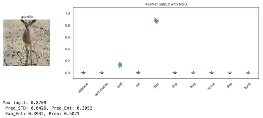
Under review as a conference paper at ICLR 2021

    Algorithm 1: Training step in NeuBoots.
    Input :Dataset D; epochs T ; blocks S; index function u; learning rate ρ.
1   Initialize neural network parameter φ(0) and set n := |D|.
2   for t ∈ {0, . . . , T − 1} do
                              (t)     (t) i.i.d.
3        Sample α(t) = {α1 , . . . , αS } ∼ Hα
                     (t)       (t)      (t)
4        Replace wα = {αu(1) , . . . , αu(n) }
                                       (t)
5         Update φ(t+1) ← φ(t) − nρ hwα , ∇φ L(Gφ (α(t) ), D)i    φ=φ(t)
                                                                           .

    Algorithm 2: Prediction step in NeuBoots.
    Input : Data point X∗ ∈ Rp ; number of bootstrap samples B.
1                                     b ∗ (·) = Gφ (X∗ , ·).
    Evaluate the feed-forward network G
2   for b ∈ {1, . . . , B} do
                          i.i.d.             (b)
3       Generate α(b) ∼ Hα and evaluate yb∗ = G   b ∗ (α(b) ).

    Note that the solution of equation 3.2 coincides with the solution of equation 3.1 provided the
    uniqueness of the solution of equation 3.1. Then, for a feature of interest X∗ , we can theoretically show
    that G(X
         b ∗ , w) = fbw (X∗ ) holds almost surely (see Theorem A.1 in the supplementary materials),
    where fbw = arg minf ∈N Λ[f ](w). This means that the bootstrapped sample is exactly matched to
    the conventional target that shares the same weight.

    3.3     N EU B OOTS A LGORITHM

    Despite of its exactness, Φ[G] receives a supplementary input w from high-dimension space Wn , so
    its practical implementation and optimization via equation 3.2 would be hurdled for massive-sized
    data sets. To overcome this problem, we utilize a block bootstrapping procedure to reduce the
    dimension of the supplementary input. The proposed procedure asymptotically converges towards the
    same target distribution where the conventional non-block bootstrap converges to, and under some
    mild regularity conditions, this result is rigorously proven in the supplementary materials.

    Block bootstrapping For m ∈ N, we write [m] := {1, . . . , m}. Let I1 , . . . , IS denotes the index
    sets of exclusive S blocks. We allocate the index of training data [n] to each block I1 , . . . , IS by
    the stratified sampling to balance among classes. Let index function u : [n] → [S] denotes such
    assignment i.e. u(i) = s if i ∈ Is . Then, for some weight distribution Hα on WS , we impose the
    same value of weight on all elements in a block such as, wi = αu(i) , where α = {α1 , . . . , αS } ∼ Hα
    for i ∈ [n], and we define wα = {αu(1) , . . . , αu(n) }. Similar with the vanilla version of the
    GBS, setting Hα = S × Dirichlet(1, . . . , 1) induces a block version of the RWB, and imposing
    Hα = Multinomial(S; 1/S, . . . , 1/S) results in a block nonparametric bootstrap. We also remark
    that the Dirichlet distribution with a uniform parameter
                                                           Pn      of one can be easily approximated by
    independent exponential distribution. That is, zi / k=1 zk ∼P      Dirichlet(1, . . . , 1) for independent
                                                                         n
    and identically distributed zi ∼ Exp(1). Due to the fact that i=k zk /n ≈ 1 by the law of large
    number for a moderately large n, n−1 ×{z1 , . . . , zn } approximately follows the Dirichlet distribution.
    This property is convenient in a sense that we do not need to consider the dependence structure
    in w, and simply generate independent samples from Exp(1) to sample the bootstrap weight. We
    use this block bootstrap as a default of the NeuBoots in sequel. Theoretically, the block bootstrap
    asymptotically converges to the non-blocked bootstrap as the number of blocks S increases as
    n → ∞; see Theorem A.2 in the supplementray materials.

    Training step Thanks to the block bootstrapping, the input of the resulting generator func-
    tion G is α of which dimension is reduced from n to S. Thus, we evaluate the generator by
    Gφ (X, α) = Mβ⊕βα ◦ (Fθ (X) ⊕ α) and Φ[Gφ ] receives an input wα . Note that ∇φ Φ[Gφ ](wα ) =
    hwα , ∇φ L(Gφ (α), Dtrain )i. Then we can optimize equation 3.2 through the gradient descent by
    a Monte Carlo approximation. At every epoch, we randomly update the wα , and the expectation

                                                        4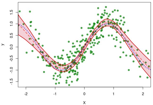
Under review as a conference paper at ICLR 2021

Figure 3.2: Two examples with different regression funtions. 95% confidence band of the regression
mean from the NeuBoots with 10,000 bootstrap samples (the first column). 95% credible bands of
the regression mean from the GP (the second column) and from the MCDrop (the third column).
Each red dashed line indicates the mean, and the blue dotted lines show the true regression function.

in equation 3.2 can be approximated by the average over the sampled weights. Considering the
stochastic gradient descent (SGD) algorithms to update the network parameter φ gradually via mini-
batch sequence {Dk : Dk ⊂ Dtrain }K  k=1 , we plug mini-batch size of wα,k = {αu(i) : Xi ∈ Dk } in
equation 3.2 instead of full-batch size of wα without changing α. Note that each element of wα is
not used repeatedly during the epoch, so the sampling and replacement procedures in Algorithm 1
are conducted once at the beginning of epoch.

Feature-Adaptive NeuBoots Modern neural networks can have different size of feature vector
according to the data. For example, ResNet or DenseNet have a smaller size of the feature vector in
CIFAR than ImageNet. In that case, a large block size S in NeuBoots can degrade the performance of
the networks. Furthermore, fitting the hyperparamter S is another painful task. Hence we additionally
propose feature-adaptive NeuBoots that removes hyperparameter S in the Algorithm 1. Recall the
decomposition f = Mβ ◦ Fθ in Section 3.2. Then, instead of choosing an arbitrary number of blocks,
we take S equals the dimension of the output of Fθ , and set Gφ (X, wα ) = Mβ (Fθ (X) wα ),
where φ = (θ, β) and denotes an elementwise multiplication. For a stable training, we utilize a
simple heuristic babysitting i.e. initially, we train a model by setting wα as one vector for t < TBS
epoch, and then we apply NeuBoots training. Consequently, these modifications show significant
improvement in calibration and active learning (see Section 4.2 and 4.3).

Prediction step After training network Gφ , for the prediction, let a data point X∗ be given and
                     b ∗ (·) = Gφ (X∗ , ·). Then we can generate bootstrapped predictions by plugging
obtain the generator G
  (1)       (B)
α ,...,α        in the generator G
                                 b ∗ , as described in Algorithm 2. Note that the algorithm evaluates the
network from the scratch for only once to obtain the generator G b ∗ , while the traditional bootstrapping
needs repetitive feed-forward propagations. Hence it brings a computational advantage of the
proposed method compared to Gal and Ghahramani (2016), which requires multiple numbers of
feed-forward evaluations for the sampling of outputs. To check this empirically, we measure the
inference time by ResNet-34 between NeuBoots and MCDrop on the test set of CIFAR-10 with
V-100 GPUs. NeuBoots predicts B = 100 bootstrapping in 1.9s whereas MCDrop takes 112s for
100-times sampling.

3.4   I LLUSTRATIVE E XAMPLE : N ONPARAMETRIC R EGRESSION

To validate the empirical properties of the proposed method, we estimate 95% confidence band
for nonparametric regression function by using the NeuBoots, and compare it with credible bands
evaluated by Gaussian Process (GP) regression based on a radial basis kernel and MCDrop (Gal
and Ghahramani, 2016). We use a MLP, which contains 3 hidden-layers with 500 hidden nodes for
each layer, to model the generator of the NeuBoots. We adopt Algorithm 1 to train the neural net
for 2000 epochs. Two illustrative examples are considered in Figure 3.2. The NeuBoots shows a

                                                    5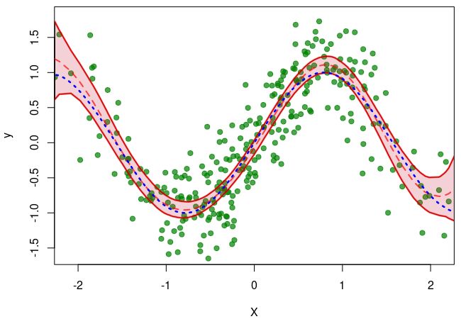
Under review as a conference paper at ICLR 2021

similar interval estimation with the GP, and more reliable confidence interval than MCDrop. We
derive the confidence intervals with same number of samples, which shows NeuBoots can evaluate a
valid confidence band, and the evaluated confidence band is comparable with the credible band of the
Bayesian GP regression. Of course, the bootstrap distribution is not a posterior, so the interpretation
of the confidence band cannot be the same with that of the Bayesian counterpart, but they surprisingly
look similar. On the other hand, even though the MCDrop theoretically approximates the Bayesian
GP regression, the resulting credible band is non-smooth and inconsistent with the shape of its target.
At the end of the feature support, the credible band of the MCDrop is clearly narrower compared to
the NeuBoots and the GP.
Furthermore, the NeuBoots is obviously scalable com-
pared to the classical GP, since the conventional GP
requires a n × n matrix inversion that demands O(n3 )          15 min      Sparse GP
                                                                           NeuBoots
computational complexity, and its computation is prac-
tically infeasible for large-sized data sets. Instead, we      10 min

compare the NeuBoots with a sparse approximation of
the GP proposed by Snelson and Ghahramani (2006),                5 min
and this approximated GP considers a small number,               3 min
                                                                 1 min
say m, of pseudo data points. Then, its computational
                                      3          2
complexity can
             √   be  reduced  to O(m    ) + O(m    n), and             500    5000     20000 40000
we set m = n. Figure 3.1 compares the computation                                    n
times of the NeuBoots and the GP, and the results show
that the NeuBoots is significantly faster than the sparse Figure 3.1: Comparison of computational
GP regression.                                             time for the sparse GP and the NeuBoots.

4     E MPIRICAL S TUDIES

In this section, we conduct the empirical studies of NeuBoots for uncertainty quantification and its
applications. We apply NeuBoots to out-of-distribution experiments, confidence estimation, and
active learning on the image classification tasks with deep convolutional neural networks.

4.1   O UT- OF -D ISTRIBUTION D ETECTION E XPERIMENTS

Setting As an important application of uncertainty quantification, we have applied NeuBoots to
detection of out-of-distribution (OOD) samples. At first, we train ResNet-34 for the classification task
in CIFAR-10 (in-distribution). We use the test datasets only for model evaluation. Then, we evaluate
the performance of NeuBoots for OOD detection in the SVHN (out-of-distribution). For each model
and dataset, we tune hyperparameters in the training phase using in-distribution samples to keep the
fairness of our method. In the evaluation phase, we use a logistic regression based detector which
outputs a confidence score for given test sample to discriminate OOD samples from in-distribution
dataset. To evaluate the performance of the detector, we measure the true negative rate (TNR) at 95%
true positive rate (TPR), the are under the receiver operating characteristic curve (AUROC), the area
under the precision-recall curve (AUPR), and the detection accuracy. For comparison, we examine the
baseline method (Hendrycks and Gimpel, 2017), ODIN (Liang et al., 2018), and Mahalanobis (Lee
et al., 2018). For our method, we tune whole hyperparameters using a separate validation set, which
consists of 1,000 images from in-distribution and out-distribution, respectively. After the training, we
estimate the following four statistics regarding logit vectors: the max of predictive mean vectors, the
standard deviation of logit vectors, expected entropy, and predictive entropy, which can be computed
by the sampled output vectors of NeuBoots. Based on these statistics, similar to Ma et al. (2018); Lee
et al. (2018), we tune the weights of logistic regression detector using nested cross-validation within
the validation set, where the label is annotated positive for in-distribution sample and annotated
negative for out-distribution sample.

Results Table 1 shows NeuBoots and feature-adaptive NeuBoots significantly outperform the
baseline method Hendrycks and Gimpel (2017) and ODIN (Liang et al., 2018) without any calibration
technique in OOD detection. Furthermore, with the input pre-processing technique studied in Liang
et al. (2018), NeuBoots is superior to Mahalanobis (Lee et al., 2018) in almost metrics, which employs
both the feature ensemble and the input pre-processing for the calibration techniques. This validates

                                                   6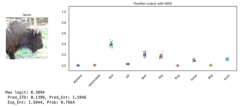
Under review as a conference paper at ICLR 2021

                                                TNR                     Detection     AUPR      AUPR
                        Method                                AUROC
                                            at TPR 95%                  Accuracy       In        Out
                        Baseline                 32.47        89.88      85.06         85.4     93.96
                         ODIN                    86.55        96.65      91.08        92.54     98.52
                      Mahalanobis                54.51        93.92      89.13        91.54     98.52
                       NeuBoots                  91.66        97.18      94.75        95.07     98.54
                      NeuBoots-FA                89.40        97.26      93.80        93.97     98.86
                Mahalanobis + Calibration        96.42        99.14      95.75        98.26     99.6
                 NeuBoots + Calibration          99.00        99.14      96.52        97.78     99.68

Table 1: The comparison NeuBoots and Baseline (Hendrycks and Gimpel, 2017), ODIN (Liang et al.,
2018), and Mahalanobis (Lee et al., 2018) on OOD detection. NeuBoots-FA means feature-adaptive
NeuBoots. We train ResNet-34 on CIFAR-10, and SVHN is used as OOD. All values are percantages
and the best results are indicated in bold.

               Data         Model       Metric     Baseline    MCDrop     NeuBoots-FA         NeuBoots-BS
                                        ACC         95.12       95.18         94.89              95.11
                          ResNet-34
                                        ECE          3.21        3.33          3.02              3.86
                                        ACC         94.11       94.07         93.36              94.17
             CIFAR-10    ResNet-110
                                        ECE          4.46        3.96          1.96              1.69
                                        ACC         94.87       95.05         93.98              94.92
                          DenseNet
                                        ECE          3.20        2.72          2.91              2.16
                                        ACC         77.88       78.33         77.54               79
                          ResNet-34
                                        ECE          7.86        7.45          9.58              12.14
                                        ACC         72.85       73.63         71.70              73.02
            CIFAR-100    ResNet-110
                                        ECE         16.58       14.89          6.3                8.0
                                        ACC         75.39       76.21         74.28              76.43
                          DenseNet
                                        ECE         12.67        9.12          1.28              3.82

Table 2: Comparison of the accuracy (ACC) and the ECE on CIFAR and architectures. All values are
percantages and the best results are indicated in bold.

NeuBoots can discriminate OOD samples effectively. In order to see the performance change of the
OOD detector concerning the bootstrap sample size, we evaluate the predictive standard deviation
estimated by the proposed method for different B ∈ {2, 5, 10, 20, 30}. Figure B.1 illustrates that, for
in-distribution classes (top row), NeuBoots predicts with extremely low uncertainty as expected. On
the other hand, for out-distribution classes (bottom row), the proposed method predicts with increased
uncertainty. As the number of bootstrap samples B increases, the predictive standard deviation for
out-distribution classes increases, so that NeuBoots can detect OOD samples better.

4.2   C ONFIDENCE E STIMATION VIA F EATURE -A DAPTIVE N EU B OOTS

Setting We evaluate the proposed method on the confidence estimation with image classifica-
tion task. We have applied feature-adaptive NeuBoots (NeuBoots-FA) and its babysitting version
(NeuBoots-BS) to image classification tasks in CIFAR-10 and CIFAR-100 with ResNet-34, ResNet-
110 and DenseNet. The size of bootstrap samples is B = 100 for prediction, and fix the other
hyperparameters same with baseline models. All models are trained using SGD with a momentum
of 0.9, an initial learning rate of 0.1, and a weight decay of 0.0005 with the mini-batch size of 128.
We use CosineAnnealing for the learning rate scheduler. For NeuBoots-BS, we set TBS = 30. We
implement MCDrop and evaluates its performance with dropout rate p = 0.2, which is a close setting
to the original paper. For the metric, we use the expected calibration error (ECE; Naeini et al. (2015)).

Results Table 2 validates that both NeuBoots-FA and NeuBoots-BS generally show better confi-
dence estimation performances compared to baseline and MCDrop. These results show that NeuBoots
is a reliable uncertainty quantification method encouraging a classifier to have robust predictions.
Observe that NeuBoots-BS secures both accuracy and confidence estimation in the image classifica-
tion tasks. Figure 4.1 shows the reliability diagrams and confidence histograms on CIFAR-100 and
DenseNet. These plots demonstrate that NeuBoots significantly improve confidence estimation.

                                                         7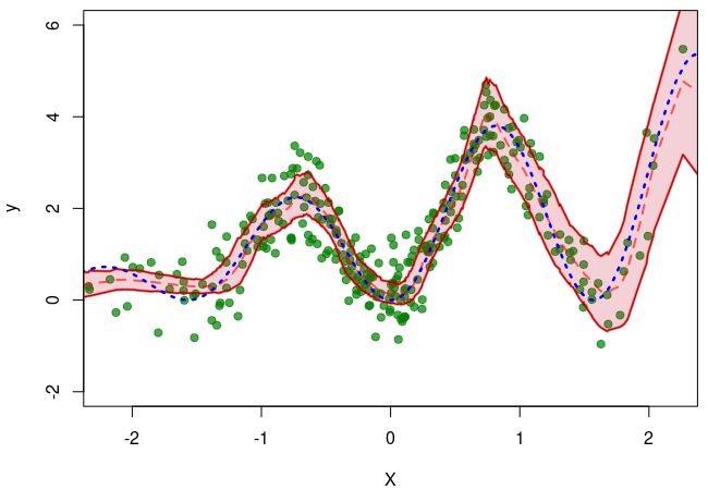
Under review as a conference paper at ICLR 2021
Figure 4.1: Comparison of reliability diagrams and confidence histograms on CIFAR-100 with
DenseNet between feature-adaptive NeuBoots (left) baseline (middle) and MCDrop (right).
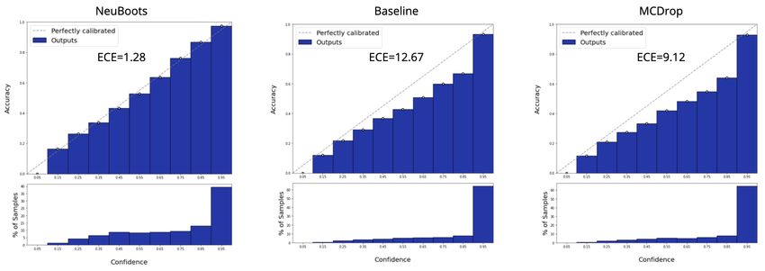
Figure 4.2: Actice learning performance on CIFAR-10 (left) and CIFAR-100 (right) with various
sampling methods. Curves are averages over five runs.
4.3 ACTIVE L EARNING
Setting We evaluate the original NeuBoots and NeuBoots-FA on the active learning with ResNet-18
architecture on CIFAR-10 and CIFAR-100. For a comparison, we consider MCDrop with entropy-
based sampling and random sampling. We follow an ordinary process to evaluate the performance
of active learning (see Moon et al. (2020) for more details). Initially, a randomly sampled 2,000
labeled images are given, and we train a model. Based on the uncertainty estimation of each model,
we sample 2,000 additional images from the unlabeled dataset and add to the labeled dataset for the
next stage. We continue this process ten times for a single trial and repeat five trials for each model.
Results Figure 4.2 shows the sequential performance improvement on CIFAR-10 and CIFAR-100.
Note that CIFAR-100 is more challenging dataset than CIFAR-10. Both plots demonstrate that
NeuBoots-FA is superior to the other sampling methods in the active learning task. NeuBoots-FA
records 71.6% accuracy in CIFAR-100 and 2.5% gap with MCDrop. Through the experiment, we
verify that NeuBoots has a significant advantage in active learning.
5 C ONCLUSION
We introduced a neural extension of bootstrap procedure, called the NeuBoots. While we applied
the NeuBoots to OOD, confidence estimation, and active learning, the NeuBoots has an attractive
potential for general purpose of neural net problems. The NeuBoots provides a valid confidence band
of a regression function, and it can be considered as a potential alternative of the GP regression under
the era of big data. One may extend the NeuBoots to recurrent neural networks or other architectures
considering the domains such as text modeling, natural language processing, and reinforcement
learning. We hope that the NeuBoots contributes to solving more challenging problems in future.
8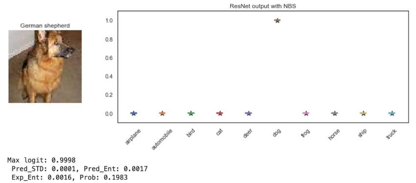
Under review as a conference paper at ICLR 2021

R EFERENCES
Carlstein, E., Do, K.-A., Hall, P., Hesterberg, T., Künsch, H. R., et al. (1998). Matched-block
  bootstrap for dependent data. Bernoulli, 4(3):305–328.
CireşAn, D., Meier, U., Masci, J., and Schmidhuber, J. (2012). Multi-column deep neural network
  for traffic sign classification. Neural networks, 32:333–338.
Cortés-Ciriano, I. and Bender, A. (2018). Deep confidence: a computationally efficient framework
  for calculating reliable prediction errors for deep neural networks. Journal of chemical information
  and modeling, 59(3):1269–1281.
Davison, A. C. and Hinkley, D. V. (1997). Bootstrap methods and their application, volume 1.
  Cambridge university press.
Efron, B. (1979). Bootstrap methods: Another look at the jackknife. The Annals of Statistics,
  7(1):1–26.
Efron, B. (1987). Better bootstrap confidence intervals. Journal of the American statistical Associa-
  tion, 82(397):171–185.
Efron, B. (2000). The bootstrap and modern statistics. Journal of the American Statistical Association,
  95(452):1293–1296.
Franke, J. and Neumann, M. H. (2000). Bootstrapping neural networks. Neural computation,
  12(8):1929–1949.
Gal, Y. and Ghahramani, Z. (2016). Dropout as a bayesian approximation: Representing model
  uncertainty in deep learning. In international conference on machine learning, pages 1050–1059.
Graves, A. (2011). Practical variational inference for neural networks. In Advances in neural
  information processing systems, pages 2348–2356.
Hall, P. (1986). On the bootstrap and confidence intervals. The Annals of Statistics, pages 1431–1452.
Hall, P. (1992). On bootstrap confidence intervals in nonparametric regression. The Annals of
  Statistics, pages 695–711.
Hall, P. (1994). Methodology and theory for the bootstrap. Handbook of econometrics, 4:2341–2381.
He, K., Zhang, X., Ren, S., and Sun, J. (2016). Deep residual learning for image recognition. In
  Proceedings of the IEEE conference on computer vision and pattern recognition, pages 770–778.
Hendrycks, D. and Gimpel, K. (2017). A baseline for detecting misclassified and out-of-distribution
  examples in neural networks. Proceedings of International Conference on Learning Representa-
  tions.
Huang, G., Liu, Z., Van Der Maaten, L., and Weinberger, K. Q. (2017). Densely connected con-
 volutional networks. In Proceedings of the IEEE conference on computer vision and pattern
  recognition, pages 4700–4708.
Kuleshov, V., Fenner, N., and Ermon, S. (2018). Accurate uncertainties for deep learning using
  calibrated regression. In International Conference on Machine Learning, pages 2796–2804.
Lakshminarayanan, B., Pritzel, A., and Blundell, C. (2017). Simple and scalable predictive uncertainty
  estimation using deep ensembles. In Advances in neural information processing systems, pages
  6402–6413.
LeCun, Y., Bottou, L., Bengio, Y., and Haffner, P. (1998). Gradient-based learning applied to
  document recognition. Proceedings of the IEEE, 86(11):2278–2324.
Lee, K., Lee, K., Lee, H., and Shin, J. (2018). A simple unified framework for detecting out-
  of-distribution samples and adversarial attacks. In Advances in Neural Information Processing
  Systems, pages 7167–7177.

                                                  9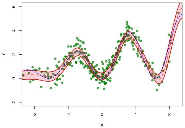
Under review as a conference paper at ICLR 2021

Liang, S., Li, Y., and Srikant, R. (2018). Enhancing the reliability of out-of-distribution image
  detection in neural networks. In 6th International Conference on Learning Representations, ICLR
  2018.
Louizos, C. and Welling, M. (2017). Multiplicative normalizing flows for variational bayesian neural
  networks. In Proceedings of the 34th International Conference on Machine Learning-Volume 70,
  pages 2218–2227. JMLR. org.
Ma, X., Li, B., Wang, Y., Erfani, S. M., Wijewickrema, S., Schoenebeck, G., Houle, M. E., Song, D.,
 and Bailey, J. (2018). Characterizing adversarial subspaces using local intrinsic dimensionality. In
 International Conference on Learning Representations.
Moon, J., Kim, J., Shin, Y., and Hwang, S. (2020). Confidence-aware learning for deep neural
 networks. In international conference on machine learning.
Naeini, M. P., Cooper, G. F., and Hauskrecht, M. (2015). Obtaining well calibrated probabilities
  using bayesian binning. In Proceedings of the... AAAI Conference on Artificial Intelligence. AAAI
  Conference on Artificial Intelligence, volume 2015, page 2901. NIH Public Access.
Nalisnick, E. and Smyth, P. (2017). The amortized bootstrap. In ICML Workshop on Implicit Models.
Newton, M. A. and Raftery, A. E. (1994). Approximate Bayesian inference with the weighted
  likelihood bootstrap. Journal of the Royal Statistical Society: Series B (Methodological), 56(1):3–
  26.
Præstgaard, J. and Wellner, J. A. (1993). Exchangeably weighted bootstraps of the general empirical
  process. The Annals of Probability, pages 2053–2086.
Reed, S., Lee, H., Anguelov, D., Szegedy, C., Erhan, D., and Rabinovich, A. (2014). Training deep
  neural networks on noisy labels with bootstrapping. arXiv preprint arXiv:1412.6596.
Rubin, D. B. (1981). The Bayesian bootstrap. The Annals of Statistics, 9(1):130434.
Shao, J. and Tu, D. (1996). The jackknife and bootstrap. Springer Science & Business Media.
Shin, M., Lee, Y., and Liu, J. S. (2020). Scalable uncertainty quantification via generative bootstrap
  sampler. arXiv preprint arXiv:2006.00767.
Smith, L. and Gal, Y. (2018). Understanding Measures of Uncertainty for Adversarial Example
  Detection. In UAI.
Snelson, E. and Ghahramani, Z. (2006). Sparse gaussian processes using pseudo-inputs. In Advances
  in neural information processing systems, pages 1257–1264.

                                                 10
Under review as a conference paper at ICLR 2021
A P ROOF OF T HEOREMS
In this section, we provide theoretical results in the main paper.
E XACTNESS OF N EU B OOTS
b is the solution of equation 3.2. For each w ∈ W, set
Theorem A.1. Suppose that G
fbw = arg min Λ[f ](w). (A.1)
f ∈N
Then, for any probability distribution Pw on W, Ew (Φ[G](w))
b = Ew (Λ[fbw ](w)). Furthermore,
if the solution in equation 3.1 is unique, it holds that G(Xi , w) = fbw (Xi ) almost surely for
b
i = 1, . . . , n.
The unique solution condition, assumed in Theorem A.1, is somewhat strong in practice, because
a large-sized neural network is over-parameterized and has multiple solutions of the loss function.
However, the NeuBoots successfully evaluates the bootstrapped neural networks in various empirical
examples that we examined in Section 4.
Proof. Note that G(w, ·) ∈ N for fixed w ∈ W and fbw is determined by equation A.1 for given
w ∈ W hence fb· ∈ G. Due to equation A.1, we have
Λ[fbw ](w) ≤ Φ[G](w),
for each G ∈ G. This means that, for a given Pw , it holds
Ew (Λ[fbw ](w)) ≤ Ew (Φ[G](w)), ∀G ∈ G. (A.2)
Also, by the definition of G,
b we have
Ew (Φ[G](w))
b ≤ Ew (Φ[fbw ](w)) a.s. (A.3)
Combining equation A.2 and equation A.3, the theorem is proved.
A SYMPTOTICS OF B LOCK B OOTSTRAP
We shall rigorously investigate asymptotic equivalence between the blocked bootstrap and the
non-blocked bootstrap. To ease the explanation for theory, we introduce some notation here. We
distinguish a random variable Yi and its observed value yi , and we assume that the feature X1 , X2 , . . .
is deterministic. the Euclidean norm is denoted by k · k, and the norm of a L2 space is denoted by
k · k2 . Also, to emphasize that the bootstrap weight w depends on n, we use wn . Let Y1 , Y2 , . . .
be i.i.d. random variables from the probability measure space (Ω, F, P0 ). We denote the empirical
probability measure by P bn := Pn δY /n, where δx is a discrete point mass at x ∈ R, and let
´ i=1 i
Pg = gdP, where P is a probability measure and g is a P-measurable function. Suppose that
√ b
n(Pn − P0 ) weakly converges to a probability measure T defined on some sample space and its
sigma field (Ω0 , F 0 ). In the regime of bootstrap, what we are interested in is to estimate T by using
some weighted empirical distribution that is P b∗ = Pn wi δY , where w1 , w2 , . . . is an i.i.d. weight
n i=1 i
random variable from a probability measure Pw . In the same sense, the probability measure acts on
the block bootstrap is denoted by Pwα . We state a primary condition on bootstrap theory as follows:
√
n(Pbn g − P0 g) → Tg for g ∈ D and P0 g 2 < ∞, (A.4)
D
where D is a collection of some continuous functions of interest, and gD (ω) = supg∈D |g(ω)| is the
envelope function on D. This condition means that there exists a target probability measure and the
functions of interest should be square-bounded.
Based on this condition, the following theorem states that the block bootstrap asymptotically induces
the same bootstrap distribution with that of non-block bootstrap. All proofs of theorems are deferred
to the supplementary material.
11Under review as a conference paper at ICLR 2021
Theorem A.2. Suppose that equation A.4 holds and {α1 , . . . , αS }T ∼ S × Dirchlet(1, . . . , 1) with
wi = αu(i) . We assume some regularity conditions introduced in the supplementary material, and
also assume S → ∞ as n → ∞. Then, for a rn such that kfb − f0 k2 = OPw (ζn rn−1 ) for any
diverging sequence ζn ,
n o n o
sup Pw rn (fbw (x) − fb(x)) ∈ U − Pwα rn (fbwα (x) − fb(x)) ∈ U → 0, (A.5)
x∈X ,U ∈B
in P0 -probability, where B is the Borel sigma algebra.
Recall that the notation is introduced in Section 3.3.
Præstgaard and Wellner (1993) showed that the following conditions on the weight distribution to
derive bootstrap consistency for general settings:
W1. wn is exchangeable
Pn for n = 1, 2, . . . .
W2. wn,i ≥ 0 and i=1 wn,i = n for all n.
´p
W3. supn kwn,1 k2,1 < ∞, where kwn,1 k2,1 = Pw (wn,1 ≥ t)dt.
W4. limλ→∞ lim supn→∞ supt≥λ t2 Pw (wn,1 ≥ t) = 0.
Pn
W5. n−1 i=1 (wn,i − 1)2 → 1 in probability.
√ b∗ b
Under W1-W5, combined with equation A.4, showed that n(P n − Pn ) weakly converges to T.
It was proven that the Dirichlet weight distribution satisfies W1-W5, and we first show that the
Dirichlet weight distribution for the blocks also satisfies the condition. Then, the block bootstrap
of the empirical process is also consistent when the classical bootstrap of the empirical process is
consistent.
Since the block bootstrap randomly assigns subgroups, the distribution of wn is exchangeable, so
the condition W1 is satisfied. The condition W2 and W3 are trivial. Since a Dirichlet distribution
with a unit constant parameter can be approximated by a pair of independent exponential random
PS PS i.i.d.
variables; i.e {z1 / i=1 zi , . . . , zS / i=1 zi } ∼ Dir(1, . . . , 1), where zi ∼ exp(1). Therefore,
S × Dir(1, . . . , 1) ≈ {z1 , . . . , zS }, if S is large enough. This fact shows that t2 Pw (wn,1 ≥ t) ≈
t2 Pz (z1 ≥ t), and it follows that Pz (z1 ≥ t) = exp(−t), so W4 is shown. The condition W5 is
trivial by the law of large number. Then, under W1-W5, Theorem 2.1 in Præstgaard and Wellner
(1993) proves that
√
n(Pb∗ − Pbn ) ⇒ T, (A.6)
n
where the convergence “⇒” indicates weakly convergence.
We denote the true neural net parameter by φ0 such that f0 = fφ0 , where f0 is the true function that
involves in the data generating process, and φb and φbw are the minimizers of the equation 3.1 for
one-vector (i.e. w = (1, . . . , 1)) and given w, respectively. This indicates that fb = fφb and fbw = fφbw .
Then, our objective function can be expressed as minimizing Pbn L(fφ (X), y) with respect to φ. We
further assume that
A1. the true function belongs to the class of neural network, i.e. f0 ∈ F.
n o n o
A2. supx∈X ,U ∈B Pw rn (fbw (x) − fb(x)) ∈ U − P0 rn (fb(x) − f0 (x)) ∈ U → 0,
in P0 -probability, where f0 is the true function that involves in the data generating process.
Pn ∂ Pn ∂
A3. Suppose that i=1 ∂φ L(fφb(Xi ), yi ) = 0, i=1 ∂φ wi L(fφbw (Xi ), yi ) = 0 for any w, and
∂
E0 [ ∂φ L(fφ0 (X), y)] = 0.
∂ √ b
A4. H is in P0 -Donsker family, where H = { ∂φ L(fφ (·), ·) : φ ∈ Φ}; i.e. n(P n g − P0 g) → Tg
b
2
for g ∈ H and P0 gH < ∞.
These conditions assume that the classical weighted bootstrap is consistent, and a rigorous theoretical
investigation of this consistency is non-existent at the current moment. However, we remark that the
main purpose of this theorem is to show that the considered block bootstrap induces asymptotically
the same result from the classical non-block bootstrap so that the use of the block bootstrap is at least
12Under review as a conference paper at ICLR 2021
asymptotically equivalent to the classical counterpart. In this sense, it is reasonable to assume that
the classical bootstrap is consistent.
Then, it follows that
n o n o
sup Pw rn (fbw (x) − fb(x)) ∈ U − Pwα rn (fbwα (x) − fb(x)) ∈ U
x∈X ,U ∈B
n o n o
≤ sup Pw rn (fbw (x) − fb(x)) ∈ U − P0 rn (fb(x) − f0 (x)) ∈ U
x∈X ,U ∈B
n o n o
+ sup Pwα rn (fbwα (x) − fb(x)) ∈ U − P0 rn (fb(x) − f0 (x)) ∈ U .
x∈X ,U ∈B
The first part in the right-hand side of the inequality converges to 0 by A1. Also, the second
part also converges to 0. That is because the empirical process of the block weighted bootstrap
is asymptotically equivalent to the classical RWB, so A2 and A3 guarantees that the asymptotic
behavior of the bootstrap solution should be consistent as the classical counterpart does.
13Under review as a conference paper at ICLR 2021
Figure B.1: Histogram of the predictive standard deviation estimated by NeuBoots on test samples
from CIFAR-10 (in-distribution) classes (top row) and SVHN (out-distribution) classes (bottom row),
as we vary bootstrap sample size B ∈ {2, 5, 10, 20, 30}.
B A DDITIONAL E XPERIMENTAL R ESULTS
In this section, we illustrate additional results of OOD detection experiments.
14Under review as a conference paper at ICLR 2021
Figure B.2: Confidence bands of the prediction of NeuBoots for bison data in TinyImageNet. The
proposed method predicts is as an out-of-distribution class with prob=0.7664.
Figure B.3: Confidence bands of the prediction of NeuBoots for gazelle data in TinyImageNet. The
proposed method predicts is as an out-of-distribution class with prob=0.5021.
Figure B.4: Confidence bands of the prediction of NeuBoots for German shepherd data in TinyIm-
ageNet. The proposed method predicts is as an in-of-distribution class dog with prob=0.1983.
15You can also read