Adaptive dictionary learning based on local configuration pattern for face recognition - EURASIP Journal on Advances in Signal Processing
←
→
Page content transcription
If your browser does not render page correctly, please read the page content below
Wei et al. EURASIP Journal on Advances in Signal Processing               (2020) 2020:20
https://doi.org/10.1186/s13634-020-00676-5
                                                                                                                EURASIP Journal on Advances
                                                                                                                         in Signal Processing

 RESEARCH                                                                                                                                           Open Access

Adaptive dictionary learning based on local
configuration pattern for face recognition
Dongmei Wei1, Tao Chen1, Shuwei Li1, Dongmei Jiang2, Yuefeng Zhao1* and Tianping Li1*

  Abstract
  Sparse representation based on classification and collaborative representation based classification with regularized
  least square has been successfully used in face recognition. The over-completed dictionary is crucial for the
  approaches based on sparse representation or collaborative representation because it directly determines
  recognition accuracy and recognition time. In this paper, we proposed an algorithm of adaptive dictionary learning
  according to the inputting testing image. First, nearest neighbors of the testing image are labeled in local
  configuration pattern (LCP) subspace employing statistical similarity and configuration similarity defined in this paper.
  Then the face images labeled as nearest neighbors are used as atoms to build the adaptive representation dictionary,
  which means all atoms of this dictionary are nearest neighbors and they are more similar to the testing image in
  structure. Finally, the testing image is collaboratively represented and classified class by class with this proposed
  adaptive over-completed compact dictionary. Nearest neighbors are labeled by local binary pattern and microscopic
  feature in the very low dimension LCP subspace, so the labeling is very fast. The number of nearest neighbors is
  changeable for the different testing samples and is much less than that of all training samples generally, which
  significantly reduces the computational cost. In addition, atoms of this proposed dictionary are these high dimension
  face image vectors but not lower dimension LCP feature vectors, which ensures not only that the information
  included in face image is not lost but also that the atoms are more similar to the testing image in structure, which
  greatly increases the recognition accuracy. We also use the Fisher ratio to assess the robustness of this proposed
  dictionary. The extensive experiments on representative face databases with variations of lighting, expression, pose,
  and occlusion demonstrate that the proposed approach is superior both in recognition time and in accuracy.
  Keywords: Collaborative representation classification, Nearest neighbors, Local configuration pattern (LCP), Statistical
  similarity, Configuration similarity

1 Introduction                                                                           Facial images are very high dimensional, which is bad
As a biological feature, the human face has been paid                                  for classification. So dimension reduction is carried out
more attention because it can be easily captured with a                                before classification. Principle component analysis (PCA)
common camera even without cooperation of the sub-                                     [1–4] has become the classic reducing dimension ap-
ject. Yet the performance of face recognition is affected                              proach and has been used widely in image processing
by the expression, illumination, occlusion, pose, age                                  and pattern recognition fields. All training images make
change, and so on. There are still some challenges in the                              up covariance matrix, and these eigenvectors corre-
field of unrestricted face recognition.                                                sponding to the bigger eigenvalues of covariance matrix
                                                                                       span the linear feature subspace. Through projecting
* Correspondence: yuefengzhao@126.com; Sdsdltp@163.com                                 high-dimensional original face images onto the low di-
1
 Shandong Provincial Engineering and Technical Center of Light                         mensional linear feature subspace, PCA performs the di-
Manipulations & Shandong Provincial Key Laboratory of Optics and Photonic              mension reduction and preserves the global structure of
Device, School of Physics and Electronics, Shandong Normal University, Jinan
250014, China                                                                          an image.
Full list of author information is available at the end of the article

                                       © The Author(s). 2020 Open Access This article is licensed under a Creative Commons Attribution 4.0 International License,
                                       which permits use, sharing, adaptation, distribution and reproduction in any medium or format, as long as you give
                                       appropriate credit to the original author(s) and the source, provide a link to the Creative Commons licence, and indicate if
                                       changes were made. The images or other third party material in this article are included in the article's Creative Commons
                                       licence, unless indicated otherwise in a credit line to the material. If material is not included in the article's Creative Commons
                                       licence and your intended use is not permitted by statutory regulation or exceeds the permitted use, you will need to obtain
                                       permission directly from the copyright holder. To view a copy of this licence, visit http://creativecommons.org/licenses/by/4.0/.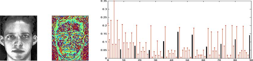
Wei et al. EURASIP Journal on Advances in Signal Processing   (2020) 2020:20                                             Page 2 of 12

   Designed as a texture descriptor originally, local binary            structured sparse representation based classification
patterns (LBP) [5] is a simple and efficient algorithm, it              [18]. In which, occlusion dictionary is not an identity
can capture the local structural features that are very im-             matrix, but is learned from data and is smaller than that
portant for human texture perception. Researches show                   of SRC. In addition, the occlusion dictionary is inde-
that LBP is discriminative and robust to illumination, ex-              pendent of the training sample as possible, so the occlu-
pression, pose, misalignment, and so on. LBP has been a                 sion is sparsely represented by the learned occlusion
popular feature extraction approach and has been used                   dictionary and can be separated from the occluded
successfully in face recognition [6–8]. Up to now, some                 image. The testing image is classified by the recovered
improved approaches based on LBP have been pre-                         non-occluded image. Ou also provided another occlu-
sented, such as complete LBP (CLBP) [9], local Gabor                    sion dictionary learning algorithm named discriminative
LBP [10], multi-scale LBP [11], and so on. Because the                  nonnegative dictionary learning, where the occlusions
intensity of the central pixel is independent to its LBP                were estimated adaptively by the reconstruction errors
value, the information embodying the relationship be-                   and weights for different pixels were learned during it-
tween pixels in the same neighborhood is lost. Guo et al.               erative processing [19]
[12] proposed the local configuration pattern (LCP) in-                    The resolution method of sparse representation vector
cluding both local structural and microscopic features.                 (or sparse solution) is another crucial issue for sparse rep-
The local structural features are represented by the pat-               resentation based on classification (SRC), which influences
tern occurrence histograms, just as LBP, and the micro-                 the recognition accuracy and recognition time. The first
scopic features are described by optimal model                          researchers, such as the above mentioned, hold the view
parameters. The microscopic configuration features re-                  that “sparsity” of the sparse representation vector is the
veal the pixel-wise interaction relationships. It has been              most crucial for SRC and paid more attention to the
proved LCP is an excellent feature descriptor. In this                  “sparsity” of sparse solution. Because l0_norm
paper, we use LCP to measure the similarities between                   minimization is NP-hard, they used l1_norm minimization
face images and finally to find neighbors of testing                    to replace l0_norm minimization as the optimal solution
image.                                                                  (the sparsest solution). But l1_norm minimization is time-
   Many researches confirmed that sparse representation                 consuming, which is bad for recognition especially in the
and collaborative representation are good at image pro-                 case of real-time identification. Ma et al [20] proposed a
cessing, such as image reconstruction, image representa-                discriminative low-rank dictionary learning, in which the
tion, and image classification. Li et al proposed an                    over-completed discriminative dictionary is composed of
effective approach called patch matching-based multi-                   series of sub-dictionaries. Atoms of each sub-dictionary
temporal group sparse representation to restore the                     are training images from the same category, so they are
missing information that should be contained in remote                  linearly correlated and all sub-dictionaries are low-rank
sensing images [13] (Patch Matching-Based Multitem-                     with a compact form. Zhang et al. [21] also regarded the
poral Group Sparse Representation for the Missing In-                   feature coding problem as the low-rank matrix learning
formation Reconstruction of Remote-Sensing Images).                     problem and researched local structure information
Yang et al. [14] regarded face recognition as a globally                among features on the image-level. Using the similarities
sparse representation problem and proposed the face                     among local features embraced in the same spatial neigh-
recognition (FR) approach known sparse representation                   borhood, an exacting joint representation of these local
based on classification (SRC), in which the over-                       features w.r.t. the codebook was founded. Zhang et al [22]
complete dictionary is formed by training face images.                  analyzed the mechanism of SRC and found that “collabor-
Subsequently, To improve the recognition accuracy with                  ation representation” among categories is the crucial fac-
occlusion, Wright et al. [15] subsequently introduced an                tor for SRC. He relaxed the demand on “sparsity” and
identity matrix to code the outlier pixels that were oc-                used l2-norm to replace l1-norm as the sparse constraint
cluded. Yang et al. [16] viewed the sparse coding as a                  condition and proposed the algorithm known collabora-
sparsity constrained robust regression problem and pro-                 tive representation based on classification with regularized
posed the robust sparse coding method. It is more ro-                   least square (CRC_RLS). Gou et al investigated deeply
bust to detect outliers than SRC. In 2010, Yang et al.                  approaches based on collaborative representation-
[17] introduced Gabor features into SRC; they projected                 classification and proposed several novel approaches of
firstly the high-dimension facial images into the lower                 classification based on collaborative representation
dimension Gabor-feature space and then used SRC to                      [23–26]. He proposed a two-phase probabilistic collab-
classify. This approach greatly decreased the size of the               orative representation-based classification [25], in
occlusion dictionary compare with that of SRC. As a re-                 which the nearest representative samples are chosen
sult, recognition-time is reduced. Ou et al. proposed an                first and then each testing sample is represented and
approach of face recognition with occlusion named                       classified by those chosen nearest samples. In Ref.
Wei et al. EURASIP Journal on Advances in Signal Processing   (2020) 2020:20                                                         Page 3 of 12

[26], the locality of data is employed to constrain the                        y ¼ Xβ                                                        ð1Þ
collaborative representation in order to represent
faithfully testing images with the nearest samples. In                  where β ¼ ½β1;1 ; β1;;2 ; ⋯; βT1;m;…;β                    ∈ℜ M1 is the
                                                                                                                 Q;1 ;⋯;βQ;mQ
this paper, we proposed a new and simple approach
based on sparse representation and LCP features. We                     representation coefficient vector.
pay our attention to the over-completed compact dic-                      Sparse representation classification firstly encodes the
tionary. Atoms of this proposed dictionary are all                      testing image by all training images according to Eq. (1)
nearest neighbors in LCP feature subspace, so struc-                    and then classifies class-by-class. Specifically, if the
tures of atoms are more similar to that of testing im-                  testing image y comes from the qth subject (class),
ages and the atoms’ number is greatly decreased                         entries of its β should be zero except for those
compared with the training images, which will im-                       associated with theqth class ideally, i.e. β ¼
prove the recognition accuracy and reduce the recog-                    ½0; ⋯; 0; βq;1 ; βq;2 ; ⋯; βq;mq ; 0; ⋯; 0T (T is transpose op-
nition time.
                                                                        eration). In fact, any entry of βcan be very small non-
  This paper is organized as follows: related theories
                                                                        zero, so the identity of y is determined by the residual
about SRC and LCP were described in Section 2. The
                                                                        between yt and its reconstruction by each class. Let βq
proposed face recognition approach using a sparse
representation-based adaptive nearest dictionary was                    ¼ ½βq;1 ; βq;2 ; ⋯; βq;mq T be the representation coefficient
described in Section 3. Experimental results were pro-                  associated with the qth class. The reconstruction of the
vided in Section 4 and conclusions were illustrated in                  test image by the qth class training samples denotes
Section 5.                                                              byyq, yq = Xqβq, the residual rq = ‖y − yq‖2 = ‖y − Xqβq‖2.
                                                                        The testing image is classified to the qth class if rq is the
2 Related                                                               minimum residual, i.e.,
2.1 Sparse representation based on classification
                                                                               identity ðyÞ ¼ arg min r q                                    ð2Þ
Assume there are M training face images from Q sub-                                                q
                                       P
                                       Q
jects, each subject has mq images, M ¼    mq . Let vq,                    How to get the representation coefficient vector from
                                                     q¼1
                                                                        Eq. (1) is crucial for sparse representation. Sparse repre-
i∈ ℜd × 1 denote the d-dimension vector stretched by the                sentation requires the dictionary to satisfyd < M, so Eq.
ith image from theqth class (subject) and yrepresent the                (1) has more than one solution. The sparest solution is
testing image vector. Let matrix Xq ¼ ½vq;1 ; ⋯; vq;mq                 generally considered as the optimal solution for classifi-
whose column vectors are the training images from the                                                             ^ is the solution
                                                                        cation. The optimal solution expressed β
qth class, X = [X1, ⋯, Xq, ⋯, XQ] ∈ ℜd × M is the set of all
                                                                        of Eq. (3), while it is a NP-hard problem.
training images.
  Yang et al. [14] proved that face recognition can be                         ^ ¼ arg min kβk s:t: Xβ ¼ y
                                                                               β              0                                              ð3Þ
regarded as sparse representation based on classification                               β
(SRC) if there were enough training face images (the
number of training face images M should be greater                        Theories of sparse representation and compressed
than the dimension of image, i.e., d < M). In this case,                sensing reveal that l0-norm minimization solution and
the testing imagey can be as the sparse linear combin-                  l1-norm minimization solution were nearly equivalent
ation of all training images, i.e.,                                     when the solution is sparse enough. So Yang [14]

    Fig. 1 Flowchart of this proposed algorithm (CRC_NLCP)
Wei et al. EURASIP Journal on Advances in Signal Processing (2020) 2020:20 Page 4 of 12
Fig. 2 Chi-BRD-distances and chi-BRD-similarities
employed l1-norm to replace l0-norm and estimated the P‐1
X
1; a≥ 0
optimal representation vector by Eq. (4) LBPP;R ¼ u g p −g c 2p ; uðxÞ ¼
p¼0
0; a < 0
^ ¼ arg min kβk
β s:t: kXβ−yk2 ≤ ε ð4Þ ð6Þ
1
β
where R is the radius of the circle neighborhood cen-
where εdenotes the error term including noisy and tered at the given pixel, P is the number of neighboring
model error, and this is the well-known sparse represen- samples spaced at regular intervals on this circle, gcis
tation based on classification (SRC). gray of the center pixel, and gp (p = 0, 1, ⋯P − 1) denotes
Zhang employed l2-norm as the sparse constraint gray of its neighboring.
condition to solve representation vector using regular- Regard the LBP as a circular binary string with P bits,
ized least square and proposed CRC_RLS algorithm the number of two bitwise transitions 0 and 1 is defined
[22], in which the representation vector can be ob- as U. If U ≤ 2, then the LBP are defined as a uniform
tained by Eq. (5) pattern, notated LBPu2P;R . Ojala et al. [5] defined the
rotation-invariant uniform patterns LBPriu2P;R :
^ ¼ arg min ky−Xβk2 þ λkβk2
β ð5Þ
β
2 2 8
P‐1
u g p −g c ; U LBPP;R ≤ 2
With regularized least squares method, the unique so- LBPP;R ¼ p¼0
riu2
ð7Þ
>
:
lution of Eq. (5) can be easily educed as β ^¼ P þ 1; otherwise
−1
ðXT X þ λIjÞ XT y, where λ is a regularization parameter LetNk denotes the occurrence of the k-pattern in-
given experientially. P
w P
h
AssumeP = (XTX + λI| )−1XT, it is clear that P is inde- cluded in LBP,N k ¼ δðLBPriu2
P;R ði; jÞ; kÞ; ðk ¼ 0; 1;
pendent of y, so P can be seen as a projection matrix de- i¼1 j¼1
cided only by training images. Just projecting y onto P, ⋯; 2P Þ, where δ(x, y) is the Dirac function. Histogram H
^ can be solved easily, β=Py.
β ^ expresses the LBP feature vector of the image.
According to sparse representation theory, the over- H ¼ ½N 1 ; ⋯N k ; ⋯; N S ð8Þ
completed dictionary should be satisfied that the num-
ber of features is greater than that of an atom. However, where S is the maximum value of LBP pattern.
face recognition is a typical small-size-sample task and Although the LBP feature vector can capture the stat-
matrix X made directly by face images could not be an istical feature of the image and is robust for illumination,
over-completed dictionary. Generally, dimension reduc- it neglects the relationship between neighboring pixels,
tion was performed before a sparse representation. which leads to wrong classification results when images
have the same LBP feature but the different gray varia-
2.2 Local configuration pattern tions between the center pixel and its neighboring pixels.
In essence, LBP feature is the histogram build by LBP Guo et.al [12]. introduced the microscopic feature (MiC)
value of all pixels in an image. LBP of the given pixel is information into LBP and proposed a local configuration
defined as follows [5]: pattern (LCP).Wei et al. EURASIP Journal on Advances in Signal Processing (2020) 2020:20 Page 5 of 12
Table 1 The description on both face databases −1
AL ¼ CL GTL GTL GL ð10Þ
Database name AR ORL
Number of class 100 40 A small probability event (NL ≤ P)is regarded as
Number of image per subject 14 10 unreliable and its model parameters are set to zero. The
PP
−1
Total number of image 1400 400 Fourier transform of AL isϕL(k), ϕ L ðkÞ ¼ aLp e− j2πkp=P
Number of training image per class 7 6 p¼0
ðk ¼ 0; ⋯; P−1Þ . MiC features consist of the amplitude
Total number of training-image 700 240
of the Fourier transform (|ϕL(k)|), denoted by ΦL.
Number of testing image per class 7 4
Total number of testing image 700 160 ΦL ¼ ðjϕ L ð0Þj; ⋯; jϕ L ðP−1ÞjÞ ð11Þ
Size of image 60 × 43 112 × 92
Appending NL to ΦL, LCP feature corresponding to L
pattern can be obtained by the Eq. (12). The LCP feature
Let A = (a0, ⋯, aP − 1) presents a parameter vector and vector of an image can be obtained by concatenating all
g = (g0, ⋯, gP − 1)presents a neighboring vector of center S LCP features, it is denoted by FLCP.
PP
−1
pixel. The central pixel can be reconstructed by ap g p , FLCP ¼½Φ1 ; N 1 ; ⋯; ΦS ; N S ð12Þ
p¼0
P
P−1
the reconstruction error j g c − ap g p jwill be minimum 3 Methods
p¼0
According to sparse representation theories, the more
when parameter vector A reaches optimum. similar the atom is to the testing sample, the sparser the
Assume there are NL pixels whose patterns are all representation vector is, and the greater recognition ac-
equal to L, let cLi ði ¼ 1; ⋯; N L Þ denote the gray value of curacy of the dictionary is.
the ith center pixel belonging to L pattern, these NL gray Let η = mq/Mdescribe the sparsity of the representa-
values made up the matrix CL ¼ðcL1 ; cL2 ; ⋯; cLN L Þ. Vector tion vector. If all classes have the same number of
gLi ¼ ðg Li;0 ; g Li;1 ; ⋯; g Li;P−1 Þ consists of the gray values of training samples, thenη = 1/Q, else minq(mq)/M ≤ η ≤
0 L 1 maxq(mq)/M, where minq(mq) and maxq(mq) are the
g1
neighboring pixels of ci , matrix GL ¼@ ⋯ A ¼
L minimum and the maximum number of training sam-
gLN L ples for each class. The representation vector is
0 L 1 sparser with the smallerη. Clearly, we want to make
g 1;0 ; ⋯; g L1;P−1
@ A ,AL ¼ ðaL ; ⋯; aL Þrepresents the ηsmall enough. There are two ways to make η
⋮ 0 P−1 smaller. One is to augment categories and the other
g N L ;0 ; ⋯; g N L ;P−1
L L
is to reduce the sample size of each class. For the
optimal parameters corresponding to the L pattern. CL,
former, it is difficult to ask more enough volunteers
AL, and GL satisfy Eq. (9)
to take face picture. So we use the second way to in-
crease the sparsity. A testing image may be not repre-
CL ¼ AL GL ð9Þ sented sufficiently if we discard randomly some
training images, which are bad for the recognition ac-
curacy. In this paper, we recommend to utilize the
With overwhelming probability NL > > P, hence the nearest neighboring images of the testing image as
matrix GL is over-determined and the optimal parameter atoms to build a dictionary so that the testing image
vector AL can be computed by the least squares. can be represented sparsely and faithfully. SRC then
Fig. 3 One face image and its LCP feature vector. a Equalized image. b LBPriu2
8;1 spectrum. c LCP feature vectorWei et al. EURASIP Journal on Advances in Signal Processing (2020) 2020:20 Page 6 of 12
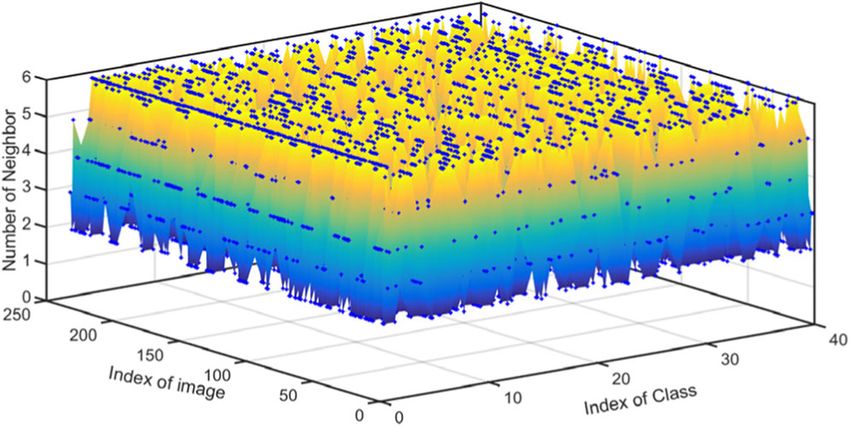
Fig. 4 Scatter diagram of nearest neighbors of training images from ORL
are performed on this proposed dictionary. We call to estimate the similarity between histograms. Hu et.al
this proposed approach for FR as “Collaborative rep- [27] proved that the distance-based chi-square is not
resentation classification based adaptive nearer- robust for partial occlusion and they may lose the co-
neighbor-dictionary” (CRC_NLCP). Figure 1 shows occurrence relations that benefit to improve the recogni-
the flowchart of this proposed algorithm. tion accuracy. Hence, he proposed a bin ratio-based
The proposed algorithm includes two stages, the distance (BRD).
first is to learn adaptively the over-completed diction- Assuming H ~ A ¼ ½uA ; ⋯uA ; ⋯; uA and H
~ B ¼ ½uB ; ⋯uB ;
1 k Q 1 k
ary, and the second stage is the SRC process. Diction-
⋯; uBQ are respectively two unit histogram vectors corre-
ary learning includes rough similarity measurement,
nearest neighbor criterion, and dictionary atom sponding the image A and image B, BRD of these two
selection. images are defined as Eq. (13):
!2
3.1 Similarity measurement X
Q X
Q
uBi uAj −uBj uAi
~ ;H
d BRD H
A
~ B
¼ ð13Þ
As the aforementioned, the LCP feature includes the
i¼1 j¼1
uAi þ uBi
statistical feature (LBP feature) described by the histo-
gram and the microscopic configuration feature de-
scribed by the parameter vector (MiC feature). So we
measure the similarity among images in these two fea- where the numerator term ( uBi uAj −uBj uAi ) embodies the
ture subspaces respectively. ratio-relations and the differences of bins included in the
same histogram, and the denominator is the standard
3.1.1 Statistical similarity term. He also proved the combination of BRD and chi-
In essence, the LBP feature vector is a frequency histo- square distance, notated as dχ 2−BRD and defined by Eq.
gram, so the chi-square distance is a good measurement (14), is superior to both them for classification.
Fig. 5 Scatter diagram of nearest neighbors of training images from ARWei et al. EURASIP Journal on Advances in Signal Processing (2020) 2020:20 Page 7 of 12
Fig. 6 Cumulative distribution function (CDF) and probability density function (PDF)of the nearer-neighbor-number. a ORL database. b
AR database
A B χ 2 BRD A B χ 2 and Chi-square-BRD-similarity (ξ) denoted by blue stars
~ ;H
dmsubsup H ~ ¼ d χ2 H~ ;H~ between one image and the others from the ORL face
B 2 X ui −ui
Q A B 2 A B
ui ui database. Clearly, ξ is more discriminative than d
~ þH
−2 H
A
~ A 3 msubsupχ −BRD . The larger ξ, the more similar two images
2
2
i¼1 ui þ uBi
are. Chi-BRD-distance between the image and itself is
ð14Þ zeros while the chi-square-BRD-similarity is infinity.
χ2 P
Q
ðuAi −uBi Þ
2
~ A; H
where d χ2 ðH ~ BÞ ¼ 2 is a chi-square dis- 3.1.2 Configuration similarity
uAi þuBi
i¼1 In the MiC feature subspace, we use Euclidean distance
tance of ðH~ ;H
A
~ Þ. For the unit length histograms, values
B
to measure the configuration similarity between two
of dmsubsup χ 2−BRD
are all very small, for example, the max- imagesx1andx2, notatingρ(x1, x2).
imum value is shown in Fig. 2 (red rhomb) is 0.025, and
differences dmsubsupχ −BRD are even smaller, which means
2
ρðx1 ; x2 Þ ¼ kΦðx1 Þ−Φðx2 Þk2 ð16Þ
dmsubsupχ −BRD has less discrimination feature and is not
2
fit to measure the statistical similarity. We defined a new
Clearly, two images are more similar if their Euclidean
statistical similarity measurement named “chi-square-
distance is smaller.
BRD-similarity” and notated as ξ to estimate the similar-
ity of images in the LBP feature subspace.
3.2 Neighboring images selection criteria
2
B χ −BRD According to Eq.(7)~(11), we can obtain unit histogram
~ ;H
ξ ðA; BÞ ¼ − log dmsubsup H ~ A
ð15Þ ~ q;i and Mic feature Φ
H ~ q;i from training imagevq, i, and
~
Hy (unit histogram of testing image) and Φ ~ y (MiC feature
of testing image). Let ξq, i andρq, idescribe respectively
Clearly, Chi-square-BRD-similarity (ξ) is the minus the statistical similarity and configuration similarity be-
logarithm of dmsubsupχ −BRD , it expands nonlinearly the
2
tween testing image y andvq, i, ξ q;i ¼ ξðH ~ y; H
~ q;i Þ can be
value range of dmsubsupχ −BRD . Figure 2 shows the chi-
2
obtained by Eq. (13) ~(15); ρq, i = ‖Φy − Φq, i‖2 can be
BRD-distance ( dmsubsupχ −BRD ) indicated by red rhombs
2
computed according to Eq. (16).
Fig. 7 The number of nearest neighbors in each categoryWei et al. EURASIP Journal on Advances in Signal Processing (2020) 2020:20 Page 8 of 12
Fig. 8 Fish-ratios of dictionaries for one testing image. a Fisher’s ratio along the different components. b Cumulative sum of fisher-ratio
P
mq compared to the face image, LCP feature vector loses
Define ξ q ¼ m1 ξ q;i as “class-average-statistical simi- much information, which are bad for SRC. We employ
q
i¼1
larity.” If ξ q;i ≥ ξ q , then the training imagevq, iis labeled as the original face image as an atom to make up the dic-
statistical neighboring. Similarly, define ‘class-average- tionary, which means all atoms of the dictionary are
P
mq these face-image-vectors labeled in the LCP subspace,
configuration similarity’ as ρq ¼ m1 ρq;i . vq, iis labeled but not LCP-feature-vectors. That is to say, sparse repre-
q
i¼1 sentation and classification are performed in face image
as configuration neighboring if ρq;i ≤ ρq . space but not in feature subspace. The experimental re-
There are two criteria to label the nearest neighbor- sults shown in the later section also verify that SRC
ing samples. One, named criterion-A, is that the nearest based on image vector is better than based on the LCP
neighboring image should be labeled as both statistical feature vector.
neighboring and configuration neighboring. The other,
named criterion-B, is that the nearest neighboring Use these training images labeled the nearest neighbor
image was labeled as either statistical neighboring or as the atoms to build the over-completed dictionary. In
configuration neighboring. Whatever criterion is used, order not to be confused with the ordinary dictionary
there must be enough training samples in each class to notated by X (defined in Section 2.1), we use R to notate
be labeled as the nearest neighbor. If not, the comple- this proposed adaptive nearest neighbor dictionary.R = [
mentary criterion, named criterion-C, must be per- R1, ⋯, Rq, ⋯, RQ], where Rq ¼ ½vq; j1 ; vq; j;…;vq; j ∈ℜ dκq (1 ≤
s
formed. In this paper, the complementary criterion j1, j2,⋯, js ≤ mq}, whose column vectors are the nearest
(criterion-C) is to sort respectively the training images neighbors selected from the qth subject’s training im-
in LBP and MiC subspace, and then keep labeling the ages. Integer κq indicates that there are κqnearest neigh-
closer ones in both two subspaces until the quantity of bor images are chosen in the qth class. Usually,
the nearest neighbor in each class reaches the require- κ1 ≠ κ2 ≠ , ⋯, ≠ κQ.
ment. Generally, the number of the nearest neighbor in
each class should be between 2 and half of the number 3.4 Assessment of the adaptive dictionary
of training images in each class. The algorithm of The over-completed dictionary greatly affects the per-
labeling the nearest neighbor is summarized as the formance of SRC. We employ Fisher’s ratio as the criter-
algorithm 1. ion to quantitatively evaluate the validity of the
dictionary. Using the within-class scatter and the
between-class scatter, Fisher’s ratio directly assesses the
class separation performance. For the q-class and p-class,
their Fisher’s ratio along the l-principal component vec-
tor direction Fq, p, l is defined
wTl Sb wl
F p;q;l ¼ ð17Þ
wTl Sw wl
3.3 Building an adaptive dictionary where Sb = (μp − μq)(μp − μq)T is the between-class
For this proposed approach, it is crucial to fast find and scatter matrix of the class p and class q, μpis the p-class
label these training samples that are more similar to the P P
mj
mean, μqis the q-class mean; Sw ¼ 12 j¼p;q ðm1 j ðx j;i −μ j
inputting testing image. So we compute the similarity in i¼1
the lower-dimension LCP feature subspace. However, Þðx j;i −μ j ÞT Þ is the within-class scatter matrix for theWei et al. EURASIP Journal on Advances in Signal Processing (2020) 2020:20 Page 9 of 12
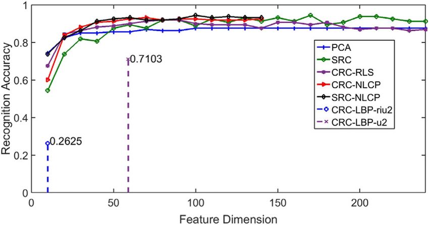
Fig. 9 The curve of recognition accuracy with feature-dimension
class p and class q, xj, i is the ith image from the jth samples have a little influence on experimental results.
class, mj is the number of the images in the class j; wl We randomly selected training samples to repeat the
is the eigenvector corresponding to the eigenvalue λl, proposed algorithm for multiple times and presented the
wlTexpress the transposition of wl. The coefficients 1/2 average result in the later of this section. All algorithms
and mj remove the interference brought by the different are coded by MATLAB 2015 and performed on the
sample size of each class. same computer with 2.6GHz CPU and 8G RAM. In this
From Eq. (17), we can see that Fp, q, l=Fq, p, l. For the paper, we never use any parallel computing or GPU.
whole dictionary, the fisher ratio along l-principal com-
ponent is defined as the mean of Fp, q, l , notated Fl: 4.1 Nearest neighbor image selection based on LCP
! features
2 X Q X Q
In order to reduce computation while retaining neigh-
Fl ¼ F p;q;l ð18Þ
QðQ−1Þ i¼1 j¼iþ1 bor attribution, we employ the rotation-invariant uni-
form pattern to compute the similarities between
Integer Q, defined in Section2.1, represents the num- images. Set P = 8, R = 1, and the length of the LCP
ber of class included in the dictionary. feature vector is 90. Figure 3 presents an example
about one face image and its LCP feature vector,
4 Results and discussion where (a) is the equalized image, (b) is the rotation-
In this section, the performance of the proposed algo- invariant uniform LBP pattern spectrum for P = 8
rithm is verified based on two standard face databases, and R = 1, and (c) is the LCP feature vector corre-
AR [28] and ORL [29]. Both face databases involve some sponding to (c). The ten groups of red vertical line ‘ ’
changes in gender, illumination, pose, expression, glass, denote the ten normalized MiC feature vectors re-
and time. The detailed data used in this paper are list in spectively, the ten black solid vertical lines describe
Table 1. the frequencies of all patterns in LBP.
This proposed adaptive dictionary is different for dif- In this paper, all images were equalized in advance
ferent testing images, so different sets of training to reduce the effects of illumination. The number of
Fig. 10 Solving times for a different number of atomsWei et al. EURASIP Journal on Advances in Signal Processing (2020) 2020:20 Page 10 of 12
Table 2 Recognition accuracy on ORL Table 4 Recognition accuracy with occlusion on AR
Best recognition rate Optimal number of features Algorithm Wears glasses Wears scarf
PCA 0.900 100 PCA 0.400 0.147
SRC 0.920 100 SRC 0.480 0.543
CRC_RLS 0.931 95 CRC_RLS 0.530 0.777
CRC_ LBP 0.706 10 CRC_NLCP 0.735 0.826
CRC_NLCP 0.975 95
We use fish-ratio defined by Eq. (17) to measure the
nearest neighbors is different for different testing im- discrimination of the dictionary. In order to compare,
ages. Figure 4 represents the scatter diagrams of the three dictionaries are created. As baseline, the first
nearer-neighbor-number for the face database ORL. dictionary, denoted by D-O, is composed by all train-
The numbers of nearest neighbor both on criterion-A ing original facial images and is stationary for all test-
and on criterion-B (given in algorithm 1) are reason- ing images; the second dictionary proposed in this
able. It is unnecessary to perform criterion-C. paper and denoted by D-p is composed by the nearest
Figure 5 represents the scatter diagrams of the neighbor facial images, and the third dictionary de-
nearer-neighbor-number for the face database AR. For noted by D-f is composed by the nearest neighbor
some images, its numbers of nearest neighbor labeled LCP feature vectors. Atom feature dimensions of both
by criterion-A are relatively small to the number of t D-O and D-p are equal to the size of the facial
classes. So the number labeled criterion-C is shown image and are much larger than the atoms’ number,
in Fig. 5. but for the dictionary D-f, the atom feature dimension
For clarity, we presented the Cumulative Distribution is dependent on the type of LBP.
Function (CDF) and Probability Density Function (PDF) According to Eq. (18), fish-ratio is defined independ-
of the nearer-neighbor-number for AR and ORL in ently along each principal component vector direction.
Fig.6, where EA and VA are mean and variance respect- We compute the fish-ratios of the three dictionaries
ively of the numbers. Obviously, the number of nearest along the bigger principal component vector directions.
neighbor labeled by criterion-A is mainly between 130 As an example, Fig. 8 presents the fish-ratios of different
and150 in AR database, it is much less than the total dictionaries for the same testing images from ORL. The
number of training images. length of the LCP feature vector is 90, so we compute
For each image in the database ORL, the number of its the fish-ratio of the first 90 principal component direc-
nearest neighbors in each class is shown in Fig. 7. It is tions for the D-f, and for the other dictionaries, the prin-
clear that the number of nearest neighbors labeled by our cipal component is less than the number of the atom.
method is almost half of that of training samples and the Figure 7b shows the cumulative sum of fish-ratio from
nearest neighbor images are distributed in all categories. the first-principal component to the given-principal
So the number of categories is not reduced, but the num- component. We can conclude that the classification
ber of atoms in each category is reduced, which reduces performance of the proposed dictionary in the paper is
the dictionary thickness and improves the sparsity. superior to the other two dictionaries.
Since the sparse dictionary requires the number of
atoms to be greater than the feature number of atoms,
4.2 Adaptive dictionary the feature number of atoms is the image resolution,
Face image is a high dimension with lots of discrim- and the image resolution is far greater than the number
inative information. But the LCP feature dimension is of images; PCA dimensionality reduction is required to
90 and LBP feature dimension is only 10 in this calculate the sparse coefficient.
paper. So much information is missed in the LCP or
LBP feature subspace, which leads to classify wrong. 4.3 Recognition accuracy
The testing image is first collaboratively represented
Table 3 Recognition accuracy without occlusion on AR with its neighbors labeled in the LCP feature subspace,
Feature dimension 10 54 120 300
PCA – 0.680 0.70.1 0.713 Table 5 Time to solve one SRV on database ORL(s)
SRC – 0.833 0.895 0.933 Method Number of atoms
CRC_RLS – 0.805 0.900 0.938 240 150 120
CRC_ LBP 0.57.0 – – – ℓ1~ℓs 0.2674 0.1775 0.1463
CRC_NLCP – 0.838 0.943 0.950 RLS 0.0077 0.0027 0.0015Wei et al. EURASIP Journal on Advances in Signal Processing (2020) 2020:20 Page 11 of 12
Table 6 Time to solve one SRV on database AR (s) mainly decided by SRV. Neither ℓ1~ℓs used in SRC nor
Method Feature Number of atoms regularized least squares (RLS) used in CRC_RLS, the
dimension time to solve SRV is mainly determined both by the
700 500 300 200
ℓ1~ℓs 100 0.4974 0.3345 0.2362 0.1982 number of dictionary atoms and by feature dimension.
Any increase in either of the two numbers will make the
200 0.5482 0.3844 0.2542 --
solution time longer. Figure 10 provided the curve of the
300 0.6890 0.4834 -- --
time spent on one SRV with the number of atoms and
400 0.8241 0.5921 -- -- feature dimensions on the database ORL.
RLS 290 0.0804 0.0408 0.0173 -- For ORL, when feature dimension equals to 95, the
450 0.0870 0.0420 -- -- time to solve one SRV with different numbers of atoms
and different methods is listed in Table 5. For database
AR, the time is given in Table 6. Experiment results
and then it is classified using its over-completed com- show that the recognition time is greatly reduced as the
pact dictionary. In this paper, we use the recognition ac- number of atoms decreases and that the RLS method is
curacy to measure the recognition performance. much faster thanℓ1~ℓs.
In addition, the number of atoms must be greater than
Number of the testing samples classified correctly the feature dimension, if not, there will be no solution.
Recognition acuracy ¼
Total number of testing samples
ð19Þ
5 Conclusion
Figure 9 shows the curve between the right recogni- Over-complete dictionaries are very important for sparse
tion rate and feature-dimension for different dictionaries representation based on classification. In this paper, we
on ORL. In which, PCA, SRC, and CRC_RLS have the presented an adaptive dictionary learning approach. We
same fixed dictionary D-O; CRC_NLCP and SRC_NLCP choose separately the training images that are closer to
have the same proposed adaptive dictionary D-p, and the the testing image from each class as the atoms to adap-
difference between them is the former used collaborative tively make up the over-complete dictionary. The pro-
representation while the later used sparse representation. posed dictionary changes with the different testing
CRC_LBP-riu2 and CRC_LBP-u2 employ the dictionary images. The closer training images are called nearest
D-f, and they employed different kinds of LBP. neighbors labeled class by class in the LCP feature sub-
To be clearer, we listed the best recognition rate and space, so atoms are more similar to the testing in struc-
the corresponding optimal feature number in Table 2. ture, which increases the recognition accuracy. In
The proposed algorithm has the greatest recognition ac- addition, the number of nearest neighboring images is
curacy reached 97.5% and a relatively small number of much smaller than that of total training images, which
features 95. CRC_LBP has the least recognition accuracy greatly reduced the recognition time. Fisher’s ratio also
rate because the number of features is too small. shows the proposed adaptive dictionary is more discrim-
Table 3 shows the recognition accuracy of the OR inatory. Experiment results also show that collaborative
database for different numbers of feature. Obviously, the representation classification based on this proposed
proposed algorithm is the best one for any dimension, adaptive nearest neighbor dictionary is excellent in rec-
and the recognition rate was improved by 0.5–4.3% ognition accuracy and in recognition time.
compared with the second best. The robustness of this To accurately and quickly identify the input testing
proposed method to occlusion (wears glasses or scarf) is images, we pay more attention to build an adaptive dic-
authenticated on AR database and the results are pre- tionary. The main idea is to find the nearest neighbors
sented in Table 4. Our algorithm recognition accuracy is of testing images in each class. If the number of training
increased by 20.5% for glass and by 4.9% for scarf. Each samples is small for certain classes, then the advantages
algorithm has different requirements for feature dimen- of this proposed algorithm will disappear. In addition,
sion, and the classification will not be performed if fea- only Euclidean distance is selected to measure MiC simi-
ture dimension is not satisfactory. larity, and we did not investigate other distance formulas
such as “cosine coefficient distance.” We also did not
4.4 Recognition time consider the image noise. In the next work, we will em-
For those approaches based on the sparse representa- ploy different distances such as “Jeffreys and Matusita
tion, recognition time consists of a solution to represen- distance,” “cosine coefficient distance,” “Canberra dis-
tation vector (SRV) and pattern matching. In this paper, tance,” and “generalized Dice coefficients” to find simi-
we employ the nearest neighbor classifier, which is the larity between images and investigate influence brought
simplest and fast, to classify. The recognition time was by noise.Wei et al. EURASIP Journal on Advances in Signal Processing (2020) 2020:20 Page 12 of 12
Abbreviations 10. W. Zhang et al., Local Gabor Binary Patterns Based on Kullback–Leibler
PCA: Principle component analysis; FR: Face recognition; LBP: Local binary Divergence for Partially Occluded Face Recognition. IEEE Signal Processing
patterns; LCP: Local configuration pattern; SRC: Sparse representation based Letters 14(11), 875–878 (2007). https://doi.org/10.1109/lsp.2007.903260
on classification; CRC_RLS: Collaborative representation based classification 11. W. Wang, F.F. Huang, J.W. Li, Face description and recognition using multi-
with regularized least square; RLS: Regularized least square; MiC: Microscopic scale LBP feature. Opt. Precis. Eng. 16(4), 696–705 (2008). https://doi.org/10.
feature; BRD: Bin ratio-based distance; SRV: Representation vector; 1080/02533839.2008.9671389
CDF: Cumulative distribution function; PDF: Probability density function 12. Y. Guo, G. Zhao, M. Pietikäinen, Local Configuration Features and
Discriminative Learnt Features for Texture Description (2014). https://doi.org/
Acknowledgements 10.1007/978-3-642-39289-4_5
The authors acknowledge the support of Shandong Province Science Key 13. X. Li, H. Shen, H. Li, et al., Patch Matching-Based Multitemporal Group
Research and Development Project (2016GGX101016) and the Innovation Sparse Representation for the Missing Information Reconstruction of
Group of Jinan (2018GXRC010). Remote-Sensing Images. IEEE Journal of Selected Topics in Applied Earth
Observations and Remote Sensing 9(8), 3629–3641 (2017). https://doi.org/
Author’s contributions 10.1109/JSTARS.2016.2533547
Dongmei Wei conceived the algorithm and designed experiments. Dongmei 14. A.Y. Yang et al., Feature selection in face recognition: A sparse
Wei, Taochen, and Shuwei Li perform the experiments. Dongmei Wei, representation perspective. IEEE Trans. Pattern Anal. Mach. Intell. (2007)
Yuefeng Zhao, and Dongmei Jiang analyzed the results. Dongmei Wei and 15. J. Wright et al., in IEEE International Conference on Automatic Face & Gesture
Tianping Li drafted the manuscript. The authors read and approved the final Recognition. Demo: Robust face recognition via sparse representation (2009).
manuscript. https://doi.org/10.1109/TPAMI.2008.79
16. M. Yang et al., in Computer Vision and Pattern Recognition. Robust sparse
Funding coding for face recognition (2011). https://doi.org/10.1109/CVPR.2011.
The work was supported by Shandong Province Science Key Research and 5995393
Development Project (2016GGX101016) and the Innovation Group of Jinan 17. M. Yang, L. Zhang, in European Conference on Computer Vision. Gabor
(2018GXRC010). Feature Based Sparse Representation for Face Recognition with Gabor
Occlusion Dictionary (2010). https://doi.org/10.1007/978-3-642-15567-3_33
Availability of data and materials 18. W. Ou, X. You, D. Tao, P. Zhang, et al., Robust face recognition via occlusion
Please contact the corresponding author for data requests. dictionary learning. Pattern Recogn. 47, 1559–1572 (2014). https://doi.org/
10.1016/j.patcog.2013.10.017
19. W. Ou, X. Luan, J. Gou, et al., Robust discriminative nonnegative dictionary
Consent for publication
learning for occluded face recognition. Pattern Recogn. Lett. 107, 41–49
Not applicable.
(2018). https://doi.org/10.1016//j.patrec.2017.07.006
20. Ma L , Wang C , Xiao B , et al. Sparse representation for face recognition
Competing interests
based on discriminative low-rank dictionary learning[C]// Computer Vision
The authors declare that they have no competing interests.
and Pattern Recognition (CVPR), 2012 IEEE Conference on. IEEE, 2012. doi:
https://doi.org/10.1109/CVPR.2012.6247977
Author details
1 21. Zhang T , Ghanem B , Liu S , et al. Low-Rank Sparse Coding for Image
Shandong Provincial Engineering and Technical Center of Light
Classification[C]// 2013 IEEE International Conference on Computer Vision
Manipulations & Shandong Provincial Key Laboratory of Optics and Photonic
(ICCV). IEEE Computer Society, 2013. doi: https://doi.org/10.1109/ICCV.2013.
Device, School of Physics and Electronics, Shandong Normal University, Jinan
42
250014, China. 2School of Electronic Information, Qingdao University,
22. L. Zhang, M. Yang, X. Feng, Sparse representation or collaborative
Qingdao, China.
representation: Which helps face recognition? 2011(5), 471–478 (2011).
https://doi.org/10.1109/ICCV.2011.6126277
Received: 8 November 2019 Accepted: 16 March 2020
23. J. Gou, B. Hou, W. Ou, Q. Mao, et al., Several robust extensions of
collaborative representation for image classification. Neurocomputing 348,
120–133.27 (2019). https://doi.org/10.1016/j.neucom.2018.06.089
References 24. J. Gou, L. Wang, Z. Yi, Y. Yuan, W. Ou, et al., Discriminative Group
1. M. Turk, A. Pentland, Eigenfaces for recognition. J. Cogn. Neurosci. 3(1), 71– Collaborative Competitive Representation for Visual Classification. IEEE
86 (1991). https://doi.org/10.1162/jocn.1991.3.1.71 International Conference on Multimedia and Expo (ICME) (2019). https://doi.
2. M. Slavković, J. Dubravka, Face recognition using eigenface approach. org/10.1109/ICME.2019.00255
Serbian Journal of Electrical Engineering 9(1), 121–130 (2012) 25. J. Gou, L. Wang, B. Hou, Y. Yuan, et al., Two-phase probabilistic collaborative
3. M.A.-A. Bhuiyan, Towards Face Recognition Using Eigenface. Int. J. Adv. representation-based classification. Expert Syst. Appl. 133, 9–20 (2019).
Comput. Sci. Appl. 7(5), 25–31 (2016) https://doi.org/10.1016/j.eswa.2019.05.009
4. Alorf A A. Performance evaluation of the PCA versus improved PCA (IPCA) in 26. J. Gou, L. Wang, Z. Yi, Y. Yuan, et al., A New Discriminative Collaborative
image compression, and in face detection and recognition[C]// Future Neighbor Representation Method for Robust Face Recognition. IEEE Access
Technologies Conference. 2017. 6(74713), 74727 (2018). https://doi.org/10.1109/ACCESS.2018.2883527
5. T. Ojala, M. Pietikäinen, T. Mäenpää, Multiresolution Gray-Scale and Rotation 27. W. Hu et al., Bin Ratio-Based Histogram Distances and Their Application to
Invariant Texture Classification with Local Binary Patterns. IEEE Transactions Image Classification. Pattern Analysis & Machine Intelligence IEEE
on Pattern Analysis & Machine Intelligence 24(7), 971–987 (2002). https:// Transactions 36(12), 2338–2352 (2014). https://doi.org/10.1109/tpami.2014.
doi.org/10.1109/tpami.2002.1017623 2327975
6. M.A. Rahim et al., Face Recognition Using Local Binary Patterns (LBP). Global 28. AR. Available from: http://rvll.ech.purdue.edu/~aleix/aleix_face_DB.html.
Journal of Computer Science & Technology (2013) 29. ORL. Available from: http://www.cam-orl.co.uk.
7. Xie S, Shan S, Chen X, et al. V-LGBP: Volume based local Gabor binary
patterns for face representation and recognition[C]. International
Conference On Pattern Recognition, 2008: 1-4 2013. doi: https://doi.org/10. Publisher’s Note
1109/ICPR.2008.4761374 Springer Nature remains neutral with regard to jurisdictional claims in
8. B. Yang, S. Chen, A comparative study on local binary pattern (LBP) based published maps and institutional affiliations.
face recognition: LBP histogram versus LBP image. Neurocomputing
120(10), 365–379 (2013). https://doi.org/10.1016/j.neucom.2012.10.032
9. Zhenhua, G., Z. Lei, and Z. David, A Completed Modeling of Local Binary
Pattern Operator for Texture Classification. Image Processing IEEE
Transactions, 2010. 19(6): p. 1657-1663.doi: https://doi.org/10.1109/TIP.2010.
2044957You can also read