A Deep Multimodal Model for Predicting Affective Responses Evoked by Movies Based on Shot Segmentation

Hindawi
Security and Communication Networks
Volume 2021, Article ID 7650483, 12 pages
https://doi.org/10.1155/2021/7650483

Research Article
A Deep Multimodal Model for Predicting Affective Responses
Evoked by Movies Based on Shot Segmentation

 Chunxiao Wang ,1,2,3 Jingjing Zhang ,1,2,3 Wei Jiang,1,2,3 and Shuang Wang1,2,3
 1
 State Key Laboratory of Media Convergence of Communication, Communication University of China, Beijing 100024, China
 2
 Key Laboratory of Acoustic Visual Technology and Intelligent Control System, Ministry of Culture and Tourism,
 Communication University of China, Beijing 100024, China
 3
 Beijing Key Laboratory of Modern Entertainment Technology, Communication University of China, Beijing 100024, China

 Correspondence should be addressed to Jingjing Zhang; zjj_cuc@cuc.edu.cn

 Received 2 July 2021; Revised 27 August 2021; Accepted 6 September 2021; Published 28 September 2021

 Academic Editor: Zhenhua Tan

 Copyright © 2021 Chunxiao Wang et al. This is an open access article distributed under the Creative Commons Attribution
 License, which permits unrestricted use, distribution, and reproduction in any medium, provided the original work is
 properly cited.
 Predicting the emotions evoked in a viewer watching movies is an important research element in affective video content analysis
 over a wide range of applications. Generally, the emotion of the audience is evoked by the combined effect of the audio-visual
 messages of the movies. Current research has mainly used rough middle- and high-level audio and visual features to predict
 experienced emotions, but combining semantic information to refine features to improve emotion prediction results is still not
 well studied. Therefore, on the premise of considering the time structure and semantic units of a movie, this paper proposes a shot-
 based audio-visual feature representation method and a long short-term memory (LSTM) model incorporating a temporal
 attention mechanism for experienced emotion prediction. First, the shot-based audio-visual feature representation defines a
 method for extracting and combining audio and visual features of each shot clip, and the advanced pretraining models in the
 related audio-visual tasks are used to extract the audio and visual features with different semantic levels. Then, four components
 are included in the prediction model: a nonlinear multimodal feature fusion layer, a temporal feature capture layer, a temporal
 attention layer, and a sentiment prediction layer. This paper focuses on experienced emotion prediction and evaluates the
 proposed method on the extended COGNIMUSE dataset. The method performs significantly better than the state-of-the-art while
 significantly reducing the number of calculations, with increases in the Pearson correlation coefficient (PCC) from 0.46 to 0.62 for
 arousal and from 0.18 to 0.34 for valence in experienced emotion.

1. Introduction sentiment analysis. Unlike short videos on social media,
 movies are much longer and can induce a rich emotional
When watching movies, audiences experience a range of response from an audience. Additionally, the rich emotional
emotions over time based on the visual and auditory in- content in movies is inherently multimodal. The complex
formation they receive. This phenomenon has been a con- interplay between audio and video modalities determines
cern of and has been studied by psychologists [1]. As people the perceived emotion. Therefore, both the complexity of the
always evaluate, select, edit, and split movies based on their film data and the dynamic interactivity of the emotional
affective characteristics, recognizing the continuous dy- content of the movie make quantifying and automatically
namic emotion evoked by movies can be used to build better predicting the emotions audiences experience a challenging
multimedia intelligent applications, such as computational problem.
affective video-in-video advertising [2] and personalized There are three different “types” of movie emotion. The
multimedia content [3], and to create automatic summaries intended emotion describes the emotional response the
and adaptive playback speed adjustment for long videos, etc. movie tries to evoke in audiences, the experienced emotion
Movies have always been one of the main objects of video describes the actual emotions felt by the viewer while

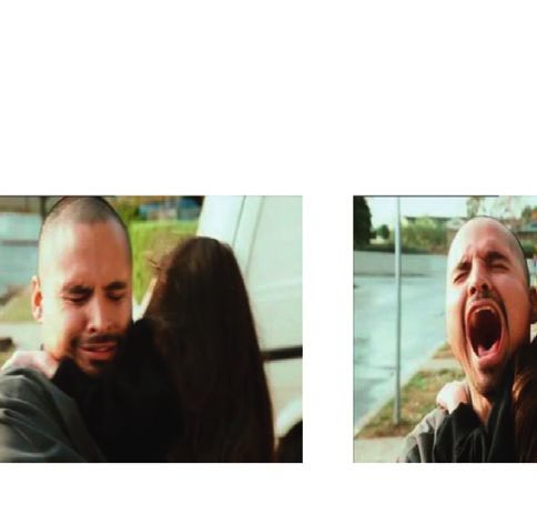
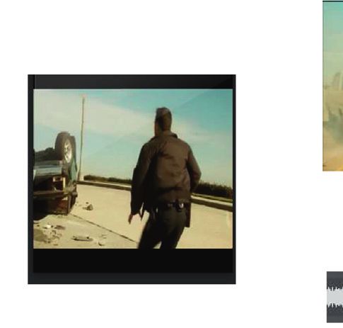
2 Security and Communication Networks

watching the movie, and the expected emotion is the ex- [6, 7, 9, 10] need to extract image content and optical flow
perienced emotion expected over a population [4]. Re- information from each frame of movies, which has high
searchers have combined existing models of affective computational complexity. Goyal et al. [6] proposed splitting
psychology to measure emotional responses, such as di- all movies into nonoverlapping 5-second samples after a
mensional and categorical approaches. The dimensional frequency response analysis of the intended and experienced
method has been used in most predictive studies [5–10] emotion labels to find a suitable unit for affective video
because the dimensional method constituted by arousal and content analysis. These methods use 5 s subclip-level aver-
valence dimensions can effectively represent the emotions aging features without considering the temporal and semantic
elicited by pictures, videos, sounds, etc. [11]. In particular, structure of the movies. There are two temporal structure
Hanjalic and Xu [12] use the arousal and valence dimensions levels of movies, shots and scenes. As the shot is the minimal
to measure the intensity and type of feeling or emotion that a visual unit of a movie [14], a multimodal prediction model
user experiences while watching a video. Malandrakis et al. based on video shot segmentation is proposed in this paper.
[4] proposed a database with continuous valence-arousal This paper focuses on experienced emotion prediction
scale annotation of intended and experienced emotions over and evaluates the proposed method on the extended
a continuous time, in which valence and arousal are an- COGNIMUSE dataset [4, 15]. First, the movies were divided
notated in the range of [−1, 1] by several subjects. The closer into short clips by shot boundary detection. Then, the audio
the valence is to 1, the more pleasant the emotions that the and visual features of each shot clip were extracted and
audience feels, and the closer it is to −1, the more negative combined with shot-based audio-visual feature represen-
the emotions that the audience feels. The closer the arousal is tation, as we define in Section 2. Finally, the shot-level audio-
to 1, the more active the audience is, and the closer it is to −1, visual features were fed into our multimodal deep model to
and the more passive the audience is. When both are closer predict the evoked emotion. This method obtained a sig-
to 0, the audience feels more neutral. Based on this modeling nificantly better result than the state-of-the-art while sig-
method, we can measure the emotions that audiences ex- nificantly reducing the number of calculations, with
perience as a range of emotions over time by continuous increases in Pearson correlation from 0.46 to 0.62 for arousal
valence-arousal scale annotation. in experienced emotion and from 0.18 to 0.34 for valence in
 For predicting the intended or experienced emotion on a experienced emotion. Interestingly, we found that the fea-
continuous valence-arousal scale, Malandrakis et al. [4] ture combination method based on shot fragments can
proposed a supervised learning method to model the con- significantly improve the performance of the method in [9].
tinuous affective response by independently using hidden The experimental results show that considering the temporal
Markov models in each dimension. Goyal et al. [6] proposed structure and semantic units of movies is of great signifi-
a mixture of experts- (MoE-) based fusion model that dy- cance to predicting experiential emotions.
namically combines information from audio and video
modalities for predicting the dynamic emotion evoked in 2. Shot Audio-Visual Feature Representation
movies. Sivaprasad et al. [7] presented a continuous emotion
prediction model for movies based on long short-term To consider a movie’s temporal structure and semantic unit,
memory (LSTM) [13] that models contextual information the variation in audio and visual information in subclips,
while using handcrafted audio-video features as input. Joshi and to reduce the high computational complexity of the
et al. [8] proposed a method to model the interdependence feature extraction process, a multimodal shot audio-visual
of arousal and valence using custom joint loss terms to feature representation was proposed as follows.
simultaneously train different LSTM models for arousal and
valence prediction. Thao et al. [9] presented a multimodal
approach that uses pretrained models to extract visual and 2.1. Video Subset Segmentation Based on Shot Boundary
audio features to predict the evoked/experienced emotions Detection. A shot is a sequence of frames recorded by the
of videos. Thao et al. [10] presented AttendAffectNet, a same camera and is the minimal visual unit of the movie
multimodal approach based on the self-attention mecha- [16]. The semantic information in one shot clip does not
nism that can find unique and cross-correspondence con- change much, but there are apparent changes in one 5 s clip,
tributions of features extracted from multiple modalities. as shown in Figure 1. The semantic variation in the 5-s clip
However, these methods usually do not take into account the increases the difficulty of model learning, so we believe that
temporal structure or semantic units of the film, ignore the the segmentation of the video shot subset can obtain higher
changes in the audio-visual information in the subclip, and accuracy in experienced emotion prediction.
have high computational complexity in the feature extrac- Sidiropoulos et al. [17] jointly exploited low-level and
tion process. high-level features automatically extracted from visual and
 Because experienced emotion prediction is more com- auditory channels, possessing better shot boundary seg-
plicated than intended emotion prediction, most researchers mentation, so this method was used to obtain shot subset
have focused on intended emotion prediction. In 2019, Thao segmentation of movies in this paper. The average value of
et al. [9] used the same features and models to predict the arousal/valence labels of all frames in each shot was used
intended or experienced emotion, and this was chosen as the as the emotion label for each shot subclip, similar to the
baseline of this paper. For predicting the emotion on a emotion label for the 5 s clips in previous studies [6–10],
continuous valence-arousal scale over time, some methods giving us approximately 5902 samples.

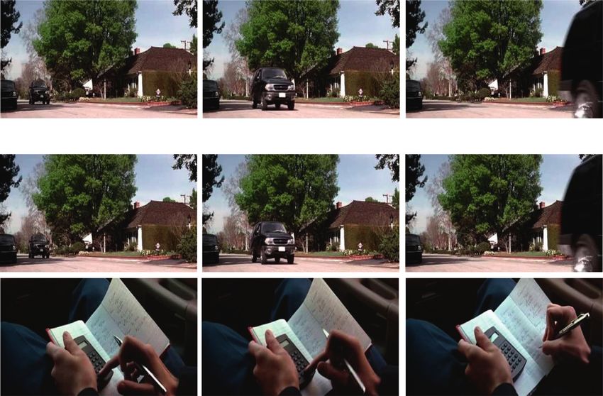
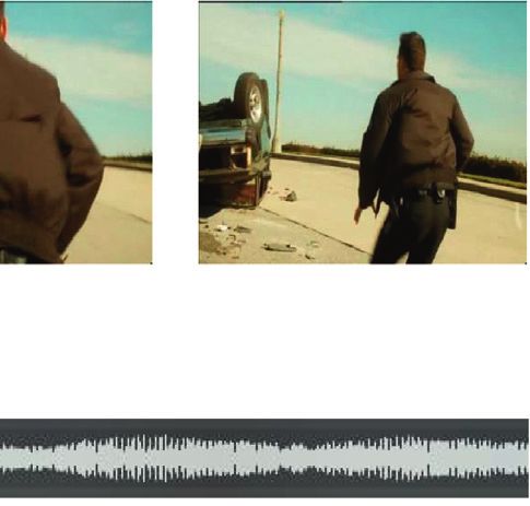
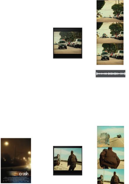
Security and Communication Networks 3

 Shot clip

 Shot1

 5s clip

 Shot2

 Figure 1: 5 s clip versus shot clip. There is little change in the semantic information in the shot clip compared to the 5 s clip.

2.2. Multimodal Emotion Features Extraction. As is known, [14] to extract the person features, and (4) ResNet50 [23]
the combined effect of the audio-visual messages of movies pretrained on the Places dataset [24] on keyframe images to
evokes emotional responses in the audience, and we hy- obtain place features. Finally, these aspects were combined
pothesize that the comprehensive effect of audio-visual into a visual feature representation of each shot clip suitable
information can be approximated by the interaction of for learning the temporal variation in the visual information
semantic units, so the extracted features need to have the in shot subclips.
ability to describe the interaction of each semantic unit in the As we know, the movie’s audio may be speech, music, or
movies. In previous studies [6–10], a global average feature sound effects, etc. But since the duration of a shot clip is too
extracted from each 5 s clip was widely used, ignoring the short, the audio of each shot subset does not have complete
change in the audio-visual information of each subclip. semantic information. To effectively describe the charac-
Therefore, to capture the interaction of each semantic unit teristics of various types of sounds, audio features were
from the audio and visual information of each shot clip, a extracted using the OpenSMILE toolkit [25] and a pre-
targeted method for extracting and combining the audio and trained VGGish model [26], as in AttendAffectNet [10]. For
visual information features of each shot clip was designed as OpenSMILE feature extraction, the configuration file
follows. “emobase2010” in the INTERSPEECH 2010 paralinguistics
 First, three keyframes of equal time intervals and one challenge [27] was used to extract 1,582 features from each
audio file in .wav format were obtained from each shot audio of the shot subset with default parameters. The
subset, as shown in Figure 2. These three keyframes cor- extracted feature set included low-level descriptors, in-
responded to the beginning, development, and end of the cluding the jitter, loudness, pitch, mel frequency cepstral
visual information of each shot clip. coefficients (MFCCs), mel filter bank, line spectral pairs with
 To consider semantic units and reduce computational their delta coefficients, functionals, duration in seconds, and
complexity, this method needed to distinguish high-level the number of pitch onsets [28]. For VGGish feature ex-
semantic elements and to replace the extraction of the traction, the pretrained VGGish network on the AudioSet
optical flow information. Thus, inspired by [16], four aspects dataset [29] was used. For each 0.96-second audio segment,
were used to represent the shot: action, face, person, and 128-d audio features were obtained, and the extracted fea-
place. Specifically, this paper utilizes (1) a partial temporal tures and overall parts were calculated to obtain the ele-
action detection model based on Fast-RCNN NonLocal- mentwise averaging to finally obtain a 128-feature vector for
I3D-50 [14] pretrained on the AVA dataset [18] to obtain the each movie shot excerpt to describe the mid-level and high-
action features, (2) a multitask cascaded convolutional level characteristics of audio. Finally, we obtained the
network (MTCNN) [19] to detect the faces in each keyframe keyframe-level visual and shot-level acoustic features.
and InceptionResnetV1 [20] to extract features of the face,
(3) a cascade region-based convolutional neural network (R-
CNN) [21] that was trained with the B-box annotations in 2.3. Shot Segment Level Features. In this paper, the keyframe-
MovieNet [14] based on the detection codebase MMDe- level visual features and the shot-level audio features are
tection [22] to detect the people in each keyframe and a combined into shot-level features that are suitable for de-
ResNet50 [23] trained with the cast annotations in MovieNet scribing the interaction between semantic units in the audio-

4 Security and Communication Networks

 Keyframe1 Keyframe2 Keyframe3

 audio file

 Movie Keyframe1 Keyframe2 Keyframe3

 audio file

 Shot clips Keyframes & audio
 Figure 2: Preprocessing operation of the shot fragment data.

visual information of each shot segment. The process of keyframes were averaged as a shot visual feature
feature processing is shown in Figure 3. Aci , Fai , Pei , Pli . For the auditory features, the 1582-di-
 For visual features, the keyframes of the shot mensional features extracted by the OpenSMILE tool and
Si , i ∈ [1, N] were denoted as Kij , j ∈ [1, 3]. For all four the 128-dimensional features extracted by pretrained
types of features of each keyframe, the action, face, person, VGGish were directly concatenated and combined as the
and place features were denoted in turn as acoustic features of the shot. Then, the shot-level visual
 AcKij , FaKij , PeKij , PlKij , i ∈ [1, N] , j ∈ [1, 3]. To extract feature was concatenated with the shot-level auditory fea-
action features, person detection of each keyframe using a ture, and the feature was normalized as a shot-level audio-
cascade R-CNN [21] was performed first, next a spatial- visual feature Aci , Fai , Pei , Pli , Vggi , Opi of shot i.
temporal action detection model was used, and then a 2048-
dimensional action feature vector of one person for each
keyframe was obtained, denoted as AcKij . Then, the ele-
 3. Multimodal Model for Emotion Prediction
mentwise averaging of AcKij , j ∈ [1, 3] was calculated to The emotion evoked in an audience is related to the audio-
obtain the shot-level action feature AcKi . When there were visual information received at the current moment and the
no people in the keyframe, a 2048 zero vector was set as its emotional state reached previously. For predicting the ex-
action features. There could be multiple faces or people in perienced emotion of viewers, the definition of the problem
each keyframe, so after the number of faces and people in all needs to be clarified. Given n shot clips, i.e., s1 , s2 , . . . , sn ,
keyframes was counted, the number of faces and people in and (n − 1) labels, denoted y1 , y2 , . . . , yn−1 , the n − th label
each keyframe with the calculated feature was set to 3. yn of the n − th shot clip sn needed to be predicted. A feature
Therefore, to extract the facial feature, facial detection was set xi � Aci , Fai , Pei , Pli , Vggi , Opi was used to represent
performed first, and 512-dimensional feature vectors for shot si . Therefore, this question translated to a nonlinear
each of the three faces in each keyframe were extracted and autoregressive exogenous problem. Given the n-d driving
then concatenated to obtain a 1582-d facial feature vector series, i.e., x1 , x2 , . . . , xn ∈ Rfd ×n , where fd is the di-
FaKij . If the number of faces in the keyframe was less than 3, mension of the shot-level features of shot si , and the previous
the feature of each undetected face was set to a 512-d zero values of the target series y1 , y2 , . . . , yn−1 with
vector. The process of extracting the person features was yi ∈ [−1, 1], nonlinear mapping was needed to learn to
similar to that of the facial features, but each person had a predict the current emotion value yn :
feature vector of 256, so a 768-d person feature vector PeKij
was obtained. For the place feature, a 2048-d vector PlKij was n � F y1 , . . . , yn−1 , x1 , . . . , xn ,
 y (1)
extracted for each keyframe. Finally, all four features were
concatenated as a visual feature representation for each where F(·) is a nonlinear mapping function that needs to be
keyframe. To simplify the operation, the features of the three learned.

Security and Communication Networks 5

 pre-trained
 Fast-RCNN
 NonLocal- Actionfeats
 I3D-50

 3 pre-trained c Face1feats
 keyframes Inception o Face2feats
 3 faces Resnet V1 n Face3feats

 Action Face

 Detector Detector

 Person Place

 Detector

 pre-trained
 Placefeats
 ResNet50
 3 persons

 c Person1feats
 Shot pre-trained
 o Person2feats
 ResNet50
 n Person3feats

 Opensmile Opensmilefeats

 audio
 Pre-trained
 vggishfeats
 VGGish

 Figure 3: Extraction of vision and audio features of a shot.

 To solve this problem, an LSTM model incorporating a inf � σ Wi x1f , . . . , xnf + bi 
temporal attention mechanism is proposed in this paper.
Specifically, four components are included: a nonlinear fnf � σ Wf x1f , . . . , xnf + bf ,
multimodal feature fusion and dimensionality reduction
layer, a temporal feature capture layer, a temporal attention gnf � tanh Wg x1f , . . . , xnf + bg ,
 (2)
layer, and a sentiment prediction layer, as shown in onf � σ Wo x1f , . . . , xnf + bo ,
Figure 4.
 cnf � fnf ⊙ c(n−1)f + inf ⊙ gnf ,
 h1nf � onf ⊙ tanh cnf 
3.1. Feature Fusion and Dimensionality Reduction.
Inspired by the basic structure of the encoder-decoder [30], where Wi , Wf , Wg , and Wo and bi , bf , bg , and bo are the
an encoder f1 (·) was proposed to capture the nonlinear parameters to learn and σ and ⊙ are a logistic sigmoid
dimensionality reduction in each feature sequence in the function and elementwise multiplication, respectively.
feature set xi � Aci , Fai , Pei , Pli , Vggi , Opi and to then xnf ∈ Aci , Fai , Pei , Pli , Vggi , Opi , so LSTM could be used
obtain the dimensionality reduction data h1i � f1 (Aci ), f1 to capture long-term dependencies of feature series to de-
(Fai ), f1 (Pei ), f1 (Pli ), f1 (Vggi ), f1 (Opi )}. f1 (·) is a scribe the interaction between high-level semantic features.
nonlinear activation function that could be LSTM or Then, all dimensionality reduction features were concate-
something else. An LSTM unit was used as f1 (·) in this nated as hicon , so we obtain hicon � f1 (Aci ) ⊕ f1 (Fai ) ⊕
paper, and the update of the LSTM unit can be summarized f1 (Pei ) ⊕ f1 (Pli ) ⊕ f1 (Vggi ) ⊕ f1 (Opi )}, where ⊕ is the
as follows: concatenation operators. Batch normalization [31] was used

6 Security and Communication Networks

 Actionfeats
 Facefeats batch-level
 c
 vision & audio Personfeats o Actionfeats
 LST LST
 features extractor Placefeats n LSTM2_Ot
 M M
 Opensmilefeats
 Shot VGGishfeats LSTM

 Audio Facefeats LST LST
 M M Content

 LSTM
 Temporal Attn
 Actionfeats
 LST LST FC
 Facefeats Personfeats
 M M
 vision & audio Personfeats Predict
 c FC
 features extractor Placefeats o B Tan value
 LSTM
 n N F h
 Opensmilefeats Softmax
 Shot c LST LST C
 VGGishfeats c
 o Placefeats M M
 Movie a Tanh
 n
 Audio t
 LSTM e
 Query
 LST LST
 Opensmilefeats M M
 Actionfeats
 Facefeats LSTM2_h0
 vision & audio Personfeats LSTM
 features extractor Placefeats
 Shot LST LST
 Opensmilefeats VGGishfeats
 M M
 VGGishfeats
 Audio LSTM
 Six concat

 Two-layer LSTM

 Figure 4: A model for arousal and valence prediction separately.

to normalize the feature data by recentering and rescaling, as Skt � WT2 tanh W1 LSTM2 (5)
 h0 ; LSTM2 Ot ,
shown in
 bs−1
 0 hicon − E bs−1 hicon exp Skt 
 h2 � �������0 . (3) αkt � . (6)
 hicon + ε ni�1 Sit
 The parameters that need to be learned are WT2 and W1 ,
 where αkt is the attention weight measuring the importance
3.2. Temporal Feature Capture. To simulate the effects of of the k-th temporal feature at time t. Equation (6) is a
current and previous audio-visual information on audi- softmax function that ensures that all the attention weights
ences, the features h2 of shots were fed to two layers of LSTM sum to 1.
to incorporate the time dependencies of the shot features, Then, the temporal feature LSTM2 Ot changes to
each with a hidden size of m units, as in Figure 4. In addition,
in this paper, m was set to 30. Therefore, after the two LSTM LSTM2O t � αkt LSTM2 Ot . (7)
layers, we could obtain LSTM2 Ot and LSTM2 h0 as
follows:
 LSTM2 Ot � σ Wio δLSTM1 hLSTM1
 t + bio + Whg ht−1 + bho , 3.4. Sentiment Value Prediction. Finally, we need to obtain
 the predicted value of each shot clip. Because the range of
 LSTM2 h0 � LSTM2 Ot ⊙ tanh LSTM2 Ct values of the valence and arousal is [−1, 1], we put LSTM2O t
 (4) passing through a fully connected layer with one unit output
 first and then through a tanh layer, as shown in Figure 4. The
where the input of the second layer of LSTM is the hidden
 calculation process is as
state hLSTM1
 t of the first layer multiplied by the dropout
δLSTM1 and δLSTM1 is a Bernoulli random variable. Wio , bio , Predict value � tanh W3 LSTM2O t . (8)
Whg , and bho are parameters that need to be learned.
LSTM2 Ot and LSTM2 h0 are the output and hidden states Additionally, W3 is a learnable parameter. For simplicity,
of the second LSTM layer, respectively. the bias term was omitted.

3.3. Temporal Attention. To adaptively learn the influence 3.5. Loss Function. Two loss functions, Loss 1 (as in equation
weights of different temporal features on this paper’s task, we (9)) and Loss 2 (as in equation (10)), were chosen and
introduce the temporal attention mechanism. We assign compared in our experiments.
LSTM2 h0 to Query and substitute LSTM2 Ot into For the loss function, Loss1 was defined as the mean
Content, as shown in Figure 4. Therefore, squared error (MSE) of prediction:

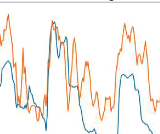
Security and Communication Networks 7

 1 n had ten cells. For LSTM, a fixed sequence length equal to 5
 Loss1 � Valuepred,i − Valueground,i , (9) and 64 hidden units were used.
 n i�1
 As shown in Table 1, under the same model and
where n is the total number of shot clips of the validation set, hyperparameter settings, the PCC of the shot-based pre-
Valuepred,i is the predicted value for the i − th shot clip, and diction of the experienced arousal is 0.13 larger than that of
Valueground,i is the ground truth of the i − th shot clip. Loss2 the 5 s-segment-based, and the MSE is approximately 0.01
was defined as litter than that of the 5 s-segment-based. However, the MSE
 of the experienced valence prediction based on the shot
 Loss2 � loss1 + 1 − p Valuepred,i , Valueground,i , (10) segment is 0.01 larger than that of the prediction based on
 the 5 s segment, while the PCC of the experienced valence is
where p is the Pearson correlation coefficient (PCC), 0.006 larger than that of the 5 s segment. Therefore, shot-
computed from the predicted arousal/valence values and the based segmentation is more favorable to the experienced
ground truth. arousal prediction task than 5 s segmentation. For the ex-
 perienced valence prediction task, shot-based segmentation
4. Experiments can obtain a better PCC even with a slightly larger MSE.
4.1. Dataset. As in existing research [4, 6–10], the extended
COGNIMUSE dataset [4, 15], which consists of twelve half- 4.4. Implementation Details. For separate arousal and va-
hour additional Hollywood movie clips, was used. This lence prediction, the model was trained using Adam opti-
dataset has the intended and experienced emotion labels at mization with learning rates of 0.01 for arousal and 0.05 for
the frame level. Emotion is represented by continuous valence. Both momenta were set to 0.005, without weight
arousal and valence values in the range [−1, 1]. This paper decay, and two losses (Loss 1 and Loss 2) were separately
focused mainly on experienced emotion, which is equivalent applied. The models were trained for 500 epochs, each batch
to evoked emotion and was described in terms of valence size was 128, and the early stopping patience was 70 epochs.
and arousal values computed as the average of twelve an- For the LSTM, the fixed sequence length was set to 5, and
notations. For comparison with previous work, the results both had 30 hidden units. All models were implemented in
for intended emotions were reported, representing the in- Python 3.6 with PyTorch 1.4 and were run on an NVIDIA
tention of the filmmakers, and were annotated in terms of GTX 2080ti.
valence and arousal values, computed as the average of three
annotations done by the same expert at the frame level. In
both cases, the emotion values (valence and arousal), which 5. Results and Analysis
ranged between −1 and 1, were quantized into shot emotion 5.1. Comparison with State-of-the-Art Results. As experi-
labels as defined in Section 2.1. All movies in the extended enced emotion prediction is more difficult than intended
COGNIMUSE dataset were used, including two animated emotion prediction, most researchers have focused on
movies, namely, “Ratatouille” and “Finding Nemo.” intended emotion prediction. In 2019, Thao et al. [9] used
 the same features and models to predict intended or ex-
4.2. Evaluation Metrics. To evaluate our proposed method, perienced emotion, respectively, and this was chosen as the
leave-one-out cross-validation was used, and the MSE and baseline in this paper. Therefore, the model was trained and
PCC between the predicted values and the ground truth for validated on the experienced and intended emotion anno-
arousal/valence were chosen as our evaluation metrics, as in tations in the COGNIMUSE dataset for effective compari-
[9, 10]. For leave-one-out cross-validation, we selected each son. The results are summarized in Table 2 for experienced
movie in turn as the validation set and the other movies as emotion prediction and in Table 3 for intended emotion
the training set, and the averages of all training results (MSE prediction.
and PCC) were used as the overall results. For the evaluation As shown in Table 2, the performance of our prediction
metrics, the closer the MSE was to 0 and the closer the PCC method is significantly better than that of Thao et al. [9]. The
was to 1, the better the prediction. best results are obtained for each forecasting task when
 arousal or valence is predicted with Loss1 or Loss2, re-
 spectively. In particular, the MSE of the arousal prediction
4.3. Shot Clip versus 5 s Clip. First, a preexperiment to briefly task decreases from 0.04 to 0.027, and the PCC increases
verify and compare the effectiveness of the two segmentation from 0.46 to 0.62; the MSE of the valence prediction task
methods was conducted. To simplify the experiment, this changes from 0.06 to 0.063, and the PCC improves from 0.18
part used the same features as Thao et al. [9]. We imple- to 0.34. As shown in Figures 5 and 6, the curve of the
mented a regression deformation based on the sequence predicted values always exhibits a sudden large change over
memory model [9] to predict arousal and valence. In this time. When the forecasting model does not have sufficient
model, Adam optimization [32] training was used; the fitting power, the overall curve consisting of all the forecast
learning rate of arousal and valence prediction was 0.0005; values flattens out, resulting in a small MSE and a small PCC,
the momentum was set to 0.00002, weight attenuation was which does not fit the sharp fluctuations in the curve.
not performed, and two losses (Loss 1 and Loss 2) were used Therefore, we prefer methods that give higher PCC values to
separately. The fully connected layer for feature reduction prioritize the model itself and to ensure better fitting

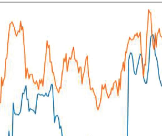
8 Security and Communication Networks

 Table 1: Comparison of the performance of the two segmentation methods.
 Experienced arousal Experienced valence
Features
 MSE PCC MSE PCC
5 s features4 (loss2) 0.0476 0.4543 0.0707 0.2145
Shot features4 (loss2) 0.0377 0.5822 0.0820 0.2203
The best result for each indicator is marked in bold.

 Table 2: Comparison of state-of-the-art results for experienced emotion prediction.
 Arousal Valence
Method
 MSE PCC MSE PCC
Thao et al. [9] 0.04 0.46 0.06 0.18
Ours (loss1) 0.0275 0.6187 0.0490 0.2828
Ours (loss2) 0.0403 0.5569 0.0632 0.3443

 Table 3: Comparison of state-of-the-art results for intended emotion prediction.
 Arousal Valence
Models
 MSE PCC MSE PCC
Malandrakis et al. [4] 0.17 0.54 0.24 0.23
Goyal et al. [6] — 0.62 ± 0.16 — 0.29 ± 0.16
Sivaprasad et al. [7] 0.08 ± 0.04 0.84 ± 0.06 0.21 ± 0.06 0.50 ± 0.14
Thao et al. [9] 0.13 0.62 0.19 0.25
Thao et al. [10] 0.124 0.630 0.178 0.572
Ours (loss1) 0.1022 0.6748 0.1654 0.3167
Ours (loss2) 0.1141 0.6582 0.1704 0.4025

performance. Therefore, Loss1 is more suitable for arousal truth in some periods. This phenomenon may mean that
prediction tasks, while is better for valence prediction. there are different ways in which the same features interact
 As shown in Table 3, our model obtains results com- with each other in various movies and that these ways of
parable to the state-of-the-art results for both arousal and interaction are affected by the specific values of the features.
valence in intended emotion prediction. For arousal-
intended emotion prediction, Sivaprasad et al. [7] obtained
the best results, with a PCC equal to 0.84 and an MSE of 0.08. 5.2. Ablation Experiments of Features. To verify the contri-
However, their data excludes the two animated movies from bution of each visual or auditory feature to the overall effect,
the COGNIMUSE dataset just as in [6]. The PCC and MSE of feature ablation experiments were conducted. This section
our method are 0.67 and 0.10, respectively, which are the was validated using the same model with the same hyper-
best results without handcrafted features. For valence- parameters as that in Section 4.4.
intended emotion prediction, Thao et al. [10] obtained the As shown in Table 4, we subtract one feature each time
best results, with a PCC of 0.57 and an MSE of 0.17. The we validate, “Action features,” “Face features,” “Person
results of our method are slightly worse, with a PCC of 0.40 features,” “Place features,” “VGGish features,” or “Open-
and an MSE of 0.17. This may be because our model is not as SMILE features,” and use only the visual and auditory
complex as theirs, but despite this, our arousal prediction features for prediction. The experimental results show that
performance surpasses theirs, indicating that our feature the contribution of each visual or auditory feature to the
combination is more effective. Compared to the model of overall arousal prediction results is generally comparable.
equal-level complexity reported by Thao et al. [9], a sig- Although the performance of prediction by visual features
nificant improvement is reported for the intended emotion alone is still worse than that by only acoustic features, they
prediction. Specifically, both arousal and valence prediction are comparable, indicating that our proposed visual features
have smaller MSE and larger PCC. have a better ability to describe arousal information. For the
 The arousal and valence dimensions of the experienced valence prediction task, the performance of prediction by
emotion of two movies, “American Beauty” and “A Beautiful auditory features alone is much higher than that of visual
Mind,” are visualized in Figures 5 and 6, respectively. features, indicating that the proposed audio feature set has a
 As shown in Figures 5 and 6, the predicted result of better ability to describe valence attributes than the visual
arousal is much better than the valence value, which means feature set. Without the features of the person, the multi-
that the nonlinear mapping function from audio-visual cues model obtains the best PCC, which is 0.37, and a slightly
to valence is more challenging to learn. There are clear worse MSE than all features for valence prediction. This may
opposite trends for the predicted arousal values and ground be because a variety of different emotions can be evoked for

Security and Communication Networks 9

 -0.2

 -0.4
 Arousal

 -0.6

 -0.8

 0 50 100 150 200 250
 Shot index

 Ground-truth
 Predicted Values

 0.4

 0.2
 Valence

 0

 -0.2

 -0.4

 0 50 100 150 200 250
 Shot index
 Ground-truth
 Predicted Values
 Figure 5: Visualization of the arousal and valence dimensions of the experienced emotion of the movie named “American Beauty.”

the videos with the same human pose and the current model performance of the time attention mechanism is signifi-
is not complex enough to differentiate it. cantly improved. Specifically, the PCC values for both
 arousal and valence emotion prediction improve from 0.574
 and 0.296 to 0.618 and 0.34, respectively. The MSE decreases
5.3. Ablation Experiments of LSTM-One-Layer Encoder. from 0.034 and 0.071 to 0.027 and 0.063, respectively, for
This section aims to validate the ability to capture the non- arousal and valence. This proves the effectiveness of the time
linear dimensionality reduction in each feature sequence in attention mechanism.
the feature set using LSTM and its contribution to the overall
arousal and valence predictions. A comparative model was
designed for feature downscaling using a fully connected layer
and for predicting arousal and value using Loss1 or Loss2. As 5.5. Computational Complexity Comparison. In the feature
shown in Table 5, the use of LSTM to capture the nonlinear extraction process, the computational complexity of visual
dimension reduction in each feature sequence in the feature features is much higher than that of audio features, and the
set has a better effect on the overall prediction performance. extraction process of auditory features in existing studies is
In particular, the MSE of the arousal prediction task decreases similar, with computational complexity on the same order of
from 0.0288 to 0.0275, and the PCC increases from 0.5826 to magnitude. Therefore, we focus on the computational
0.6187; the MSE of the valence prediction task decreases from complexity of the visual feature extraction process for
0.0751 to 0.0632, and the PCC improves from 0.3276 to comparison. As shown in Table 7, existing studies need to
0.3443. Therefore, our LSTM-one-layer encoder helps to extract every frame’s features in the video, while the number
improve the results of all tasks. of frames to be processed is reduced to 3.21% of the original
 number of frames in this paper. Optical flow information
 extraction is replaced by action feature extraction, which has
5.4. Ablation Experiments of the Time Attention Mechanism. low computational complexity and consumes less time.
In this part, we validated the performance of the time at- Therefore, this method significantly reduces the number of
tention mechanism. As shown in Table 6, the prediction calculations and time.

10 Security and Communication Networks

 0.0

 -0.2
 Arousal
 -0.4

 -0.6

 -0.8

 0 100 200 300 400
 Shot index

 Ground-truth
 Predicted Values

 0.2

 0.0
 Valence

 -0.2

 -0.4

 -0.6

 0 100 200 300 400
 Shot index

 Ground-truth
 Predicted Values
 Figure 6: Visualization of the arousal and valence dimensions of the experienced emotion of the movie named “A Beautiful Mind.”

 Table 4: Comparison of state-of-the-art results for experienced emotion prediction.
 Arousal (loss1) Valence (loss2)
Features
 MSE PCC MSE PCC
All features 0.0275 0.6187 0.0632 0.3443
 −Action features 0.0291 0.6038 0.0673 0.3259
 −Face features 0.0277 0.6136 0.0637 0.3667
 −Person features 0.0280 0.6181 0.0653 0.3726
 −Place features 0.0280 0.5981 0.0663 0.3315
 −VGGish features 0.0290 0.5952 0.0669 0.3444
 −OpenSMILE features 0.0295 0.6003 0.0666 0.3345
All_visual_features 0.0316 0.4931 0.0751 0.2694
All_audio_features 0.0297 0.6141 0.0726 0.3356
“−” indicates without the feature.

 Table 5: With or without capture changes in audio and visual feature sequences using LSTM.
 Experienced arousal (loss1) Experienced valence (loss2)
Model (with Features6)
 MSE PCC MSE PCC
Ours without LSTM 0.0288 0.5826 0.0751 0.3276
Ours 0.0275 0.6187 0.0632 0.3443

Security and Communication Networks 11

 Table 6: With or without time attention mechanism. from this website and by contacting the creators of this
 Experienced Experienced
 dataset.
Model (with Features6) arousal (loss1) valence (loss2)
 MSE PCC MSE PCC Conflicts of Interest
Ours without attention 0.0342 0.5746 0.0718 0.2964
 The authors declare that there are no conflicts of interest
Ours 0.0275 0.6187 0.0632 0.3443
 regarding the publication of this paper.

 Table 7: Computational complexity comparison. Acknowledgments
Models Number of frames Optical flow This work was supported by the Fundamental Research
Goyal et al. [6] 551112 ✓ Funds for the Central Universities (CUC19ZD005 and
Sivaprasad et al. [7] 551112 ✓ CUC200D050).
Thao et al. [9] 551112 ✓
Thao et al. [10] 551112 ✓
Ours 17706 × References
 [1] L. Fernández-Aguilar, B. Navarro-Bravo, J. Ricarte, L. Ros,
 and J. M. Latorre, “How effective are films in inducing positive
6. Conclusion and negative emotional states? A meta-analysis,” PloS one,
 vol. 14, no. 11, Article ID e0225040, 2019.
In this paper, a multimodal prediction model based on video [2] K. Yadati, H. Katti, and M. Kankanhalli, “CAVVA: compu-
shot segmentation for predicting affective responses evoked tational affective video-in-video advertising,” IEEE Transac-
by movies is presented. Unlike many existing studies, this tions on Multimedia, vol. 16, no. 1, pp. 15–23, 2013.
paper introduces the shot clip as the minimum emotion [3] D. Aditya, R. G. Manvitha, M. Samyak, and B. S. Shamitha,
prediction of the video unit and avoids the optical flow “International conference on computing system and its ap-
calculation in feature extraction. This method enables our plications emotion based video player,” Global Transitions
model to focus on analyzing each semantic unit’s audio and Proceedings, vol. 2, no. 1, 2021.
visual information in the interaction process. Therefore, the [4] N. Malandrakis, A. Potamianos, G. Evangelopoulos, and
emotion prediction task performance was significantly A. Zlatintsi, “A supervised approach to movie emotion
improved, with an increase from 0.46 to 0.62 for arousal and tracking,” in Proceeding of the IEEE international conference
 on acoustics, speech and signal processing (ICASSP), 22-27 May
from 0.18 to 0.34 for valence in experienced emotion.
 2011.
 The movie was divided into short clips by shot boundary [5] Y. Baveye, E. Dellandrea, and C. L. Chamaret, “LIRIS-AC-
detection first. Then, three keyframes were extracted from CEDE: a video database for affective content analysis,” IEEE
each shot clip. Four types of features—action, face, person, Transactions on Affective Computing, vol. 6, no. 1, pp. 43–55,
and place features—for each keyframe of each shot clip were 2015.
extracted. For each shot clip’s audio, we used the Open- [6] A. Goyal, N. Kumar, T. Guha, and S. S. Narayanan, “A
SMILE tool and a pretrained VGGish model to extract audio multimodal mixture-of-experts model for dynamic emotion
features. Then, they were combined as shot audio-visual prediction in movies,” in Proceedings of 2016 IEEE Interna-
feature representations. Finally, the shot audio-visual fea- tional Conference on Acoustics, Speech and Signal Processing
tures were fed into our deep multimodal model based on (ICASSP), 20-25 March 2016.
 [7] S. Sivaprasad, T. Joshi, R. Agrawal, and N. Pedanekar,
LSTM incorporating temporal attention to predict emotion.
 “Multimodal continuous prediction of emotions in movies
 The effects of arousal and valence predicted separately using long short-term memory networks,” in Proceedings of
were compared by using our model with two types of loss the 2018 ACM on International Conference on Multimedia
functions. Loss1 is more suitable for arousal prediction Retrieval, Yokohama Japan, 05 June 2018.
tasks, while Loss2 is better for valence prediction. In the [8] T. Joshi, S. Sivaprasad, and N. Pedanekar, “Partners in crime:
future, we will work on designing scene-level video feature utilizing arousal-valence relationship for continuous predic-
calculation methods and a better model for mapping the tion of valence in movies,” in Proceedings of the 2nd Workshop
complex changes in visual and audio information at dif- on Affective Content Analysis (AffCon 2019) co-located with
ferent temporal levels and segment levels of the movie to Thirty-Third AAAI Conference on Artificial Intelligence (AAAI
the experienced emotion. Interestingly, the feature com- 2019), Honolulu, USA, January 2019.
bination method based on shot fragments can significantly [9] H. T. P. Thao, D. Herremans, and G. Roig, “Multimodal deep
 models for predicting affective responses evoked by movies,”
improve the performance of the method in [9]. The ex-
 in Proceedings of ICCV Workshops, 27-28 Oct. 2019.
perimental results of this paper reveal the importance of [10] H. T. P. Thao, B. T. Balamurali, D. Herremans, and G. Roig,
considering the time structure and semantic unit of movies “AttendAffectNet: self-attention based networks for predict-
for experienced emotion prediction. ing affective responses from movies,” in 25th International
 Conference on Pattern Recognition (ICPR), 10-15 Jan. 2021.
Data Availability [11] R. Dietz and A. Lang, “Affective agents: effects of agent affect
 on arousal, attention, liking and learning,” in Proceedings of
The official website of the COGNIMUSE dataset is http://cog the Third International Cognitive Technology Conference, San
nimuse.cs.ntua.gr/database. The complete data are available Francisco, August 1999.

12 Security and Communication Networks

[12] A. Hanjalic and L.-Q. Xu, “Affective video content repre- Proceedings of 2017 IEEE International Conference on
 sentation and modeling,” IEEE Transactions on Multimedia, Acoustics, Speech and Signal Processing (ICASSP), 5-9 March
 vol. 7, no. 1, pp. 143–154, 2005. 2017.
[13] S. Hochreiter and J. Schmidhuber, “Long short-term mem- [30] K. Cho, B. Van Merriënboer, C. Gulcehre et al., “Learning
 ory,” Neural Computation, vol. 9, no. 8, pp. 1735–1780, 1997. phrase representations using RNN encoder-decoder for sta-
[14] Q. Huang, Y. Xiong, A. Rao, J. Wang, and D. Lin, “Movienet: a tistical machine translation,” in Proceedings of the 2014
 holistic dataset for movie understanding,” 2020. arXiv Conference on Empirical Methods in Natural Language Pro-
 preprint. cessing (EMNLP)arXiv preprint, Doha, Qatar, October 2014.
[15] A. Zlatintsi, P. Koutras, G. Evangelopoulos et al., “COGNI- [31] S. Ioffe and C. Szegedy, “Batch normalization: accelerating
 MUSE: a multimodal video database annotated with saliency, deep network training by reducing internal covariate shift,” in
 events, semantics and emotion with application to summa- Proceedings of the International Conference on Machine
 rization,” EURASIP Journal on Image and Video Processing, Learning PMLR, pp. 448–456, Lille, France, July 2015.
 vol. 2017, no. 1, pp. 1–24, 2017. [32] D. P. Kingma and B. Jimmy, “Adam: a method for stochastic
[16] A. Rao, L. Xu, Y. Xiong et al., “A local-to-global approach to optimization,” arXiv preprint, 2014.
 multimodal movie scene segmentation,” in Proceedings of the
 IEEE/CVF Conference on Computer Vision and Pattern
 Recognition, 13-19 June 2020.
[17] P. Sidiropoulos, V. Mezaris, I. Kompatsiaris, H. Meinedo,
 M. Bugalho, and I. Trancoso, “Temporal video segmentation
 to scenes using high-level audiovisual features,” IEEE
 Transactions on Circuits and Systems for Video Technology,
 vol. 21, no. 8, pp. 1163–1177, 2011.
[18] C. Gu, C. Sun, D. A. Ross et al., “Ava: a video dataset of spatio-
 temporally localized atomic visual actions,” in Proceedings of
 the IEEE Conference on Computer Vision and Pattern
 Recognition, 18-23 June 2018.
[19] K. Zhang, Z. Zhang, Z. Li, and Y. Qiao, “Joint face detection
 and alignment using multitask cascaded convolutional net-
 works,” IEEE Signal Processing Letters, vol. 23, no. 10,
 pp. 1499–1503, 2016.
[20] C. Szegedy, S. Ioffe, V. Vanhoucke, and A. Alemi, “Inception-
 v4, inception-resnet and the impact of residual connections
 on learning,” in Proceedings of the AAAI Conference on Ar-
 tificial Intelligence, vol. 31, no. 1, California, USA, February
 2017.
[21] Z. Cai and N. Vasconcelos, “Cascade r-cnn: delving into high
 quality object detection,” in Proceedings of the IEEE conference
 on computer vision and pattern recognition, 18-23 June 2018.
[22] K. Chen, “MMDetection: open mmlab detection toolbox and
 benchmark,” arXiv preprint, 2019.
[23] K. He, X. Zhang, S. Ren, and J. Sun, “Deep residual learning
 for image recognition,” in Proceedings of the IEEE conference
 on computer vision and pattern recognition, Las Vegas, NV,
 USA, 27-30 June 2016.
[24] B. Zhou, A. Lapedriza, and A. A. Khosla, “Places: a 10 million
 image database for scene recognition,” IEEE Transactions on
 Pattern Analysis and Machine Intelligence, vol. 40, pp. 1452–
 1464, 2017.
[25] F. Eyben, Real-time Speech and Music Classification by Large
 Audio Feature Space Extraction, Springer, Berlin/Heidelberg,
 Germany, 2015.
[26] S. Hershey, S. Chaudhuri, D. P. W. Ellis et al., “CNN ar-
 chitectures for large-scale audio classification,” in Proceedings
 of 2017 ieee international conference on acoustics, speech and
 signal processing (icassp), 5-9 March 2017.
[27] B. Schuller, S. Steidl, A. Batliner et al., “The INTERSPEECH
 2010 paralinguistic challenge,” in Proceedings of Eleventh
 Annual Conference of the International Speech Communica-
 tion Association, 2010.
[28] F. Eyben, F. Weninger, M. Wöllmer et al., Open-source media
 interpretation by large feature-space extraction, TU Munchen,
 Munich, Germany, 2016.
[29] J. F. Gemmeke, D. P. W. Ellis, D. Freedman et al., “Audio set:
 an ontology and human-labeled dataset for audio events,” in