Deep-learning-based image segmentation integrated with optical microscopy for automatically searching for two-dimensional materials - Nature
←
→
Page content transcription
If your browser does not render page correctly, please read the page content below
www.nature.com/npj2dmaterials

                  ARTICLE                  OPEN

                  Deep-learning-based image segmentation integrated with
                  optical microscopy for automatically searching for
                  two-dimensional materials
                  Satoru Masubuchi 1 ✉, Eisuke Watanabe1, Yuta Seo1, Shota Okazaki2, Takao Sasagawa2, Kenji Watanabe                                           3
                                                                                                                                                                   , Takashi Taniguchi1,3 and
                  Tomoki Machida1 ✉

                      Deep-learning algorithms enable precise image recognition based on high-dimensional hierarchical image features. Here, we report
                      the development and implementation of a deep-learning-based image segmentation algorithm in an autonomous robotic system
                      to search for two-dimensional (2D) materials. We trained the neural network based on Mask-RCNN on annotated optical microscope
                      images of 2D materials (graphene, hBN, MoS2, and WTe2). The inference algorithm is run on a 1024 × 1024 px2 optical microscope
                      images for 200 ms, enabling the real-time detection of 2D materials. The detection process is robust against changes in the
                      microscopy conditions, such as illumination and color balance, which obviates the parameter-tuning process required for
                      conventional rule-based detection algorithms. Integrating the algorithm with a motorized optical microscope enables the
                      automated searching and cataloging of 2D materials. This development will allow researchers to utilize a large number of 2D
1234567890():,;

                      materials simply by exfoliating and running the automated searching process. To facilitate research, we make the training codes,
                      dataset, and model weights publicly available.
                      npj 2D Materials and Applications (2020)4:3 ; https://doi.org/10.1038/s41699-020-0137-z

                  INTRODUCTION                                                                               adjusted by experts, with retuning required when the microscopy
                  The recent advances in deep-learning technologies based on                                 conditions change. To perform the parameter tuning in conven-
                  neural networks have led to the emergence of high-performance                              tional rule-based algorithms, one has to manually find at least one
                  algorithms for interpreting images, such as object detection1–5,                           sample flake on SiO2/Si substrate, every time one exfoliates 2D
                  semantic segmentation4,6–10, instance segmentation11, and image                            flakes. Since the exfoliated flakes are sparsely distributed on SiO2/
                  generation12. As neural networks can learn the high-dimensional                            Si substrate, e.g., 3–10 thin flakes in 1 × 1 cm2 SiO2/Si substrate for
                  hierarchical features of objects from large sets of training data13,                       MoS223, manually finding a flake and tuning parameters requires
                  deep-learning algorithms can acquire a high generalization ability                         at least 30 min. The time spent for parameter-tuning process
                  to recognize images, i.e., they can interpret images that they have                        causes degradation of some two-dimensional materials, such as
                  not been shown before, which is one of the traits of artificial                             Bi2Sr2CaCu2O8+δ27, even in a glovebox enclosure.
                  intelligence14. Soon after the success of deep-learning algorithms                            In contrast, deep-learning algorithms for detecting 2D materials
                  in general scene recognition challenges15, attempts at automation                          are expected to be robust against changes in optical microscopy
                  began for imaging tasks that are conducted by human experts,                               conditions, and the development of such an algorithm would
                  such as medical diagnosis16 and biological image analysis17,18.                            provide a generalized 2D material detector that does not require
                  However, despite significant advances in image recognition                                  fine-tuning of the parameters. In general, deep-learning algo-
                  algorithms, the implementation of these tools for practical                                rithms for interpreting images are grouped into two categories28.
                  applications remains challenging18 because of the unique                                   Fully convolutional approaches employ an encoder–decoder
                  requirements for developing deep-learning algorithms that                                  architecture, such as SegNet7, U-Net8, and SharpMask29. In
                  necessitate the joint development of hardware, datasets, and                               contrast, region-based approaches employ feature extraction by
                  software18,19.                                                                             a stack of convolutional neural networks (CNNs), such as Mask-
                     In the field of two-dimensional (2D) materials20–22, the recent                          RCNN11, PSP Net30, and DeepLab10. In general, the region-based
                  advent of autonomous robotic assembly systems has enabled                                  approaches outperform the fully convolutional approaches for
                  high-throughput searching for exfoliated 2D materials and their                            most image segmentation tasks when the networks are trained on
                  subsequent assembly into van der Waals heterostructures23. These                           a sufficiently large number of annotated datasets11.
                  developments were bolstered by an image recognition algorithm                                 In this work, we implemented and integrated deep-learning
                  for detecting 2D materials on SiO2/Si substrates23,24; however,                            algorithms with an automated optical microscope to search for 2D
                  current implementations have been developed on the framework                               materials on SiO2/Si substrates. The neural network architecture
                  of conventional rule-based image processing25,26, which uses                               based on Mask-RCNN enabled the detection of exfoliated 2D
                  traditional handcrafted image features, such as color contrast,                            materials while generating a segmentation mask for each object.
                  edges, and entropy23,24. Although these algorithms are computa-                            Transfer learning from the network trained on the Microsoft
                  tionally inexpensive, the detection parameters need to be                                  common objects in context (COCO) dataset31 enabled the

                  1
                   Institute of Industrial Science, University of Tokyo, 4-6-1 Komaba, Meguro-ku, Tokyo 153-8505, Japan. 2Laboratory for Materials and Structures, Tokyo Institute of Technology,
                  4259 Nagatsuta, Midori-ku, Yokohama 226-8503, Japan. 3National Institute for Materials Science, 1-1 Namiki, Tsukuba, Ibaraki 305-0044, Japan. ✉email: msatoru@iis.u-tokyo.ac.jp;
                  tmachida@iis.u-tokyo.ac.jp

                  Published in partnership with FCT NOVA with the support of E-MRS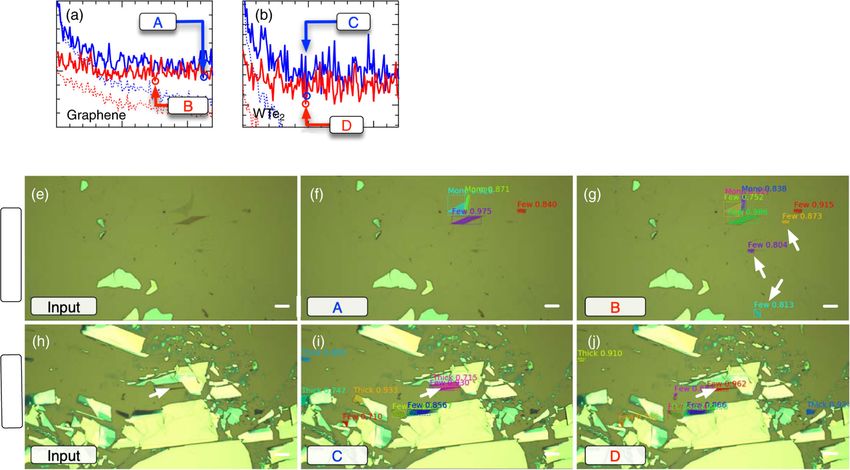
S. Masubuchi et al.
                  2
                      development of a neural network from a relatively small (~2000           the layer thickness classification, we defined three categories:
                      optical microscope images) dataset of 2D materials. Owing to the         “mono” (1 layer), “few” (2–10 layers), and “thick” (10–40 layers).
                      generalization ability of the neural network, the detection process      Note that this categorization was sufficient for practical use in the
                      is robust against changes in the microscopy conditions. These            first screening process because final verification of the layer
                      properties could not be realized using conventional rule-based           thickness can be conducted either by manual inspection or by
                      image recognition algorithms. To facilitate further research, we         using the computational post process, such as color contrast
                      make the source codes for network training, the model weights,           analysis24,38–42, which would be interfaced with the deep-learning
                      the training dataset, and the optical microscope drivers publicly        algorithms in the future works. As indicated in Fig. 1g–j, the 2D
                      available. Our implementation can be deployed on optical                 flakes are detected by the Mask-RCNN, and the segmentation
                      microscopes other than the instrument utilized in this study.            mask exhibits good overlap with the 2D flakes. The layer thickness
                                                                                               was also correctly classified, with monolayer graphene classified as
                                                                                               “mono”. The detection process is robust against contaminating
                      RESULTS                                                                  objects, such as scotch tape residue, particles, and corrugated 2D
                      System architectures and functionalities                                 flakes (white arrows, Fig. 1e, f, I, j).
                      A schematic diagram of our deep-learning-assisted optical                   As the neural network locates 2D crystals using the high-
                      microscopy system is shown in Fig. 1a, with photographs shown            dimensional hierarchical features of the image, the detection
                      in Fig. 1b, c. The system comprises three components: (i) an             results were unchanged when the illumination conditions were
                      autofocus microscope with a motorized XY scanning stage (Chuo            varied (Supplementary Movie 3). Figure 2a–c shows the deep-
                      Precision); (ii) a customized software pipeline to capture the           learning detection of graphene flakes under differing illumination
                      optical microscope image, run deep-learning algorithms, display          intensities (I). For comparison, the results obtained using
                      results, and record the results in a database; (iii) a set of trained    conventional rule-based detection are presented in Fig. 2d–f. For
                      deep-learning algorithms for detecting 2D materials (graphene,           the deep-learning case, the results were not affected by changing
                      hBN, MoS2, and WTe2). By combining these components, the                 the illumination intensity from I = 220 (a) to 180 (b) or 90 (c) (red,
                      system can automatically search for 2D materials exfoliated on           blue, and green curves, Fig. 2). In contrast, with rule-based
                      SiO2/Si substrates (Supplementary Movie 1 and 2). When 2D flakes          detection, a slight decrease in the light intensity from I = 220 (d)
1234567890():,;

                      are detected, their positions and shapes are stored in a database        to 200 (e) affected the results significantly, and the graphene
                      (sample record is presented in supplementary information), which         flakes became undetectable. Further decreasing the illumination
                      can be browsed and utilized to assemble van der Waals                    intensity to I = 180 (f) resulted in no objects being detected. These
                      heterostructures with a robotic system23. The key component              results demonstrate the robustness of the deep-learning algo-
                      developed in this study was the set of trained deep-learning             rithms over conventional rule-based image processing for
                                                                                               detecting 2D flakes.
                      algorithms for detecting 2D materials in the optical microscope
                                                                                                  The deep-learning model was integrated with a motorized
                      images. Algorithm development required three steps, namely,
                                                                                               optical microscope by developing a customized software pipeline
                      preparation of a large dataset of annotated optical microscope
                                                                                               using C++ and Python. We employed a server/client architecture
                      images, training of the deep-learning algorithm on the dataset,
                                                                                               to integrate the deep-learning inference algorithms with the
                      and deploying the algorithm to run inference on optical
                                                                                               conventional optical microscope (Supplementary Fig. 1). The
                      microscope images.
                                                                                               image captured by the optical microscope is sent to the inference
                         The deep-learning model we employed was Mask-RCNN11 (Fig.
                                                                                               server, and the inference results are sent back to the client
                      1a), which predicts objects, bounding boxes, and segmentation            computer. The deep-learning model can run on a graphics-
                      masks in images. When an image is input into the network, the            processing unit (NVIDIA Tesla V100) at 200 ms. Including the
                      deep convolutional network ResNet10132 extracts the position-            overheads for capturing images, transferring image data, and
                      aware high-dimensional features. These features are passed to the        displaying inference results, frame rates of ~1 fps were achieved.
                      region proposal network (RPN) and the region of interest                 To investigate the applicability of the deep-learning inference to
                      alignment network (ROI Align), which propose candidate regions           searching for 2D crystals, we selected WTe2 crystals as a testbed
                      where the targeted objects are located. The full connection              because the exfoliation yields of transition metal dichalcogenides
                      network performs classification (Class) and regression for the            are significantly smaller than graphene flakes. We exfoliated WTe2
                      bounding box (BBox) of the detected objects. Finally, the                crystals onto 1 × 1 cm2 SiO2/Si substrates, and then conducted
                      convolutional network generates segmentation masks for the               searching, which was completed in 1 h using a ×50 objective lens.
                      objects using the output of the ROI Align layer. This model was          Searching identified ~25 WTe2 flakes on 1 × 1 cm2 SiO2/Si with
                      developed on the Keras/TensorFlow framework33–35.                        various thicknesses (1–10 layers; Supplementary Fig. 2).
                         To train the Mask-RCNN model, we prepared annotated images               To quantify the performance of the Mask-RCNN detection
                      and trained networks as follows. In general, the performance of a        process, we manually checked over 2300 optical microscope
                      deep-learning network is known to scale with the size of the             images, and the detection metrics are summarized in Supple-
                      dataset36. To collect a large set of optical microscope images           mentary Table 1. Here, we defined true- and false-positive
                      containing 2D materials, we exfoliated graphene (covalent                detections (TP and FP) as whether the optical microscope image
                      material), MoS2 (2D semiconductors), WTe2, and hBN crystals onto         contained at least one correctly detected 2D crystal or not
                      SiO2/Si substrates. Using the automated optical microscope, we           (examples are presented in Supplementary Figs 2–7). An image in
                      collected ~2100 optical microscope images containing graphene,           which the 2D crystal was not correctly detected was considered a
                      MoS2, WTe2, and hBN flakes. The images were annotated manually            false negative (FN). Based on these definitions, the value of
                      using a web-based labeling tool37. The training was performed by         precision was TP/(TP + FP) ~0.53, which implies that over half of
                      the stochastic gradient decent method described later in                 the optical microscope images with positive detection contained
                      this paper.                                                              WTe2 crystals. Notably, the recall (TP/(TP + FN) ~0.93) was
                         We show the inference results for optical microscope images           significantly high. In addition, the examples of false-negative
                      containing 2D materials. Figure 1c–f shows optical microscope            detection contain only small fractured WTe2 crystals, which cannot
                      images of graphene, WTe2, MoS2, and hBN flakes, which were                be utilized for assembling van der Waals heterostructures. These
                      input into the neural network. The inference results shown in Fig.       results imply that the deep-learning-based detection process does
                      1g–j consist of bounding boxes (colored squares), class labels           not miss usable 2D crystals. This property is favorable for the
                      (text), confidences (numbers), and masks (colored polygons). For          practical application of deep-learning algorithms to searching for

                      npj 2D Materials and Applications (2020) 3                                    Published in partnership with FCT NOVA with the support of E-MRS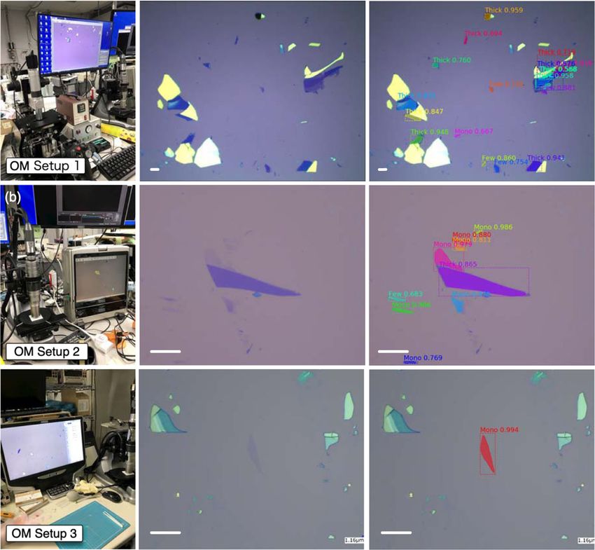
S. Masubuchi et al.
                                                                                                                                                    3
                          (a) Motorized Microscope              Deep-Learning Inference             Database
                                                          CNN Backbone ROI Align
                                                                                                                 Browse
                                                           (ResNet101)      FCN       Class

                                                                                      BBox

                                                                                                                 Design

                                                                                                         Image
                                                                                            Mask

                                                                    RPN Mask Generation

                                      Setup for deep-learning-assisted optical microscope

                                                       Input                                    Inference
                                      (d)                                      (h)
                           Graphene

                                      (e)                                      (i)
                           hBN

                                      (f)                                      (j)
                           WTe2

                                      (g)                                      (k)
                           MoS2

2D crystals, as exfoliated 2D crystals are usually sparsely                   graphene (Supplementary Table 1), both the precision and recall
distributed over SiO2/Si substrates. In this case, false-positive             were high (~0.95 and ~0.97, respectively), which implies excellent
detection is less problematic than missing 2D crystals (false                 performance of the deep-learning algorithm for detecting 2D
negative). The screening of the results can be performed by a                 crystals. We speculate that there is a difference between the
human operator without significant intervention43. In the case of              exfoliation yields of graphene and WTe2 because the mean

Published in partnership with FCT NOVA with the support of E-MRS                                       npj 2D Materials and Applications (2020) 3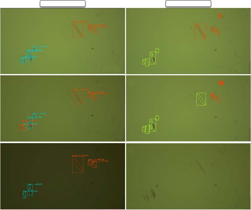
S. Masubuchi et al.
4
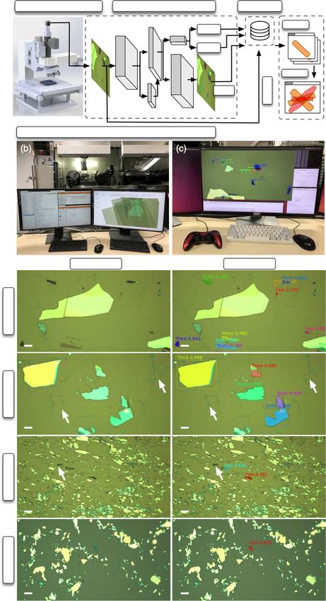
Fig. 1 Deep-learning-assisted automated optical microscope for searching for two-dimensional (2D) crystals. a Schematic of the deep-
learning-assisted optical microscope system. The optical microscope acquires an image of exfoliated 2D crystals on a SiO2/Si substrate. The
images are input into the deep-learning inference algorithm. The Mask-RCNN architecture generates a segmentation mask, bounding boxes,
and class labels. The inference data and images are stored in a cloud database, which forms a searchable database. The customized computer-
assisted-design (CAD) software enables browsing of 2D crystals, and designing of van der Waals heterostructures. b, c Photographs of (b) the
optical microscope and (c) the computer screen for deep-learning-assisted automated searching. d–k Segmentation of 2D crystals. Optical
microscope images of (d) graphene, (e) hBN, (f) WTe2, and (g) MoS2 on SiO2 (290 nm)/Si. h–k Inference results for the optical microscope
images in d–g, respectively. The segmentation masks and bounding boxes are indicated by polygons and dashed squares, respectively. In
addition, the class labels and confidences are displayed. The contaminating objects, such as scotch tape residue, particles, and corrugated 2D
flakes, are indicated by the white arrows in e, f, i, and j. The scale bars correspond to 10 µm.
Deep learning Rule-based
(a) (d)
I = 220 220
(b) (e)
180 210
(c) (f)
90 180
Fig. 2 Comparison between deep-learning and rule-based detection. Input image and inference results under illumination intensities of I =
a 220, b 180, and c 90 (arb. unit) for deep-learning detection, and I = d 220, e 210, and f 180 (arb. unit) for rule-based detection. The scale bars
correspond to 10 µm.
average precision (mAP) at the intersection of union (IOU) over where Lcls, Lbox, and Lmask are the classification, localization, and
50% mAP@IoU50% with respect to the annotated dataset (see segmentation mask losses, respectively; α – γ is the control
preparation methods below) for each material does not differ parameter for tuning the balance between the loss sets as
significantly (0.49 for graphene and 0.52 for WTe2). As demon- (α, β, γ) = (0.6, 1.0, 1.0). The class loss was
strated above, these values are sufficiently high and can be
successfully applied to searches for 2D crystals. These results Lcls ¼ log pu (2)
indicate that the deep-learning inference can be practically where p = (p0, …, pk) is the probability distribution for each region
utilized to search for 2D crystals. of interest in which the result of classification is u. The bounding
box loss Lbox is defined as
Model training X
Lbox ðtu ; v Þ ¼ smoothL1 tiu vi (3)
The Mask-RCNN model was trained on a dataset, where Fig. 3a
i2fx;y;w;hg
shows representative annotated images, and Fig. 3b shows the
annotation metrics. The dataset comprises 353 (hBN), 862 0:5x 2 ; j x j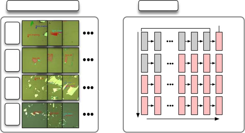
S. Masubuchi et al.
                                                                                                                                                                  5
                             (a)             Annotated Images                           (c) Training
                                                                                                             Fixed          Tuned
                                                                                                                                LR

                                         G
                                                                                                                                10-3

                                                                                            (i)
                                         hBN

                                                                                            (ii)
                                                                                                                                10-3

                                         WTe2

                                                                                            (iii)
                                                                                                                                10-4

                                                                                            (iv)
                                                                                                                                10-5
                                         MoS2

                                                                                                                               Head
                                                                                            Epoch

                                                             SiO2        # of # of Objects # of Objects # of Objects # of Objects
                             (b)              Name
                                                        Thickness (nm) Images    (Total)      (Mono)        (Few)       (Thick)
                                               BN              290           232      274              0           0            274
                                               BN              90            121      182             13          111           58
                                             Graphite          290           862     4805            1858        2081           866
                                              MoS2             290           569      839             239         523           77
                                              WTe2             290           318     1053             148         582           323
                                              Tot al                        2102     7153            2258        3297          1598

                                                   test (w/o aug.)           test (w aug.)
                             (d)                   train (w/o aug.)          train (w aug.)

                                   1.5

                                   1.0
                            Loss

                                   0.5

                                             (i)                     (ii)                    (iii)                   (iv)
                                   0.0
                                         0                20                40         60                   80          100
                                                                                     Epoch
Fig. 3 Overview of training. a Examples of annotated datasets for graphene (G), hBN, WTe2, and MoS2. b Training data metrics. c Schematic of
the training procedure. d Learning curves for training on the dataset. The network weights were initialized by the model weights pretrained
on the MS-COCO dataset. Solid (dotted) curves are test (train) losses. Training was performed either with (red curve) or without (blue curve)
augmentation.

   Instead of training the model from scratch, the model weights,                      operations were applied to the training data with a random
except for the network heads, were initialized using those                             probability online to reduce disk usage (examples of the
obtained by pretraining on a large-scale object segmentation                           augmented data are presented in Supplementary Figs 8 and 9).
dataset in general scenes, i.e., the MS-COCO dataset31. The                            Before being fed to the Mask-RCNN model, each image was
remaining parts of the network weights were initialized using                          resized to 1024 × 1024 px2 while preserving the aspect ratio, with
random values. The optimization was conducted using a                                  any remaining space zero padded.
stochastic gradient decent with a momentum of 0.9 and a weight                            To improve the generalization ability of the network, we
decay of 0.0001. Each training epoch consisted of 500 iterations.                      organized the training of the Mask-RCNN model into two steps.
The training comprised four stages, each lasting for 30 epochs                         First, the model was trained on mixed datasets consisting of
(Fig. 3c). For the first two training stages, the learning rate was set                 multiple 2D materials (graphene, hBN, MoS2, and WTe2). At this
to 10–3. The learning rate was decreased to 10–4 and 10–5 for the
                                                                                       stage, the model was trained to perform segmentation and
last two stages. In the first stage, only the network heads were
                                                                                       classification, both on material identity and layer thickness. Then,
trained (top row, Fig. 3c). Next, the parts of the backbone starting
at layer 4 were optimized (second row, Fig. 3c). In the third and                      we use the trained weights as a source, and performed transfer
fourth stages, the entire model (backbone and heads) was trained                       learning on each material subset to achieve layer thickness
(third and fourth rows, Fig. 3c). The training took 12 h using four                    classification. By employing this strategy, the feature values that
GPUs (NVIDIA Tesla V100 with 32-GB memory). To increase the                            are common to 2D materials behind the network heads were
number of training datasets, we used data augmentation                                 optimized and shared between the different materials. As shown
techniques, including color channel multiplication, rotation,                          below, the sharing of the backbone network contributed to faster
horizontal/vertical flips, and horizontal/vertical shifts. These                        convergence of the network weights and a smaller test loss.

Published in partnership with FCT NOVA with the support of E-MRS                                                     npj 2D Materials and Applications (2020) 3
S. Masubuchi et al.
6
Training curve feature values that are common to 2D materials are learnt in the
Figure 3d shows the value of the loss function as a function of the backbone network. In particular, the trained backbone network
epoch count. The solid (dotted) curves represent the test (training) weights contribute to improving the model performance on each
loss. The training was conducted either with (red curves) or material.
without (blue curves) data augmentation. Without augmentation, To investigate the improvement of the model accuracy, we
the training loss decreased to zero, while the test loss was compared the inference results for the optical microscope images
increased. The difference between the test and training losses was using the network weights from each training set. Figure 4e–h
significantly increased with training, which indicates that the shows the optical microscope images of graphene and WTe2,
generalization error increased, and the model overfits the training respectively, input into the network. We employed the model
data13. When data augmentation was applied, both the training weights where the loss value was minimum (indicated by the red/
and validation losses decreased monotonically with training, and blue arrows). The inference results in the cases of transferring only
the difference between the training and validation losses was from MS-COCO, and from both MS-COCO and 2D materials, are
small. These results indicate that when 2000 optical microscope shown in Fig. 4f, g for graphene, and Fig. 4I, j for WTe2. For
images are prepared, the Mask-RCNN model can be trained on 2D graphene, the model transferred from MS-COCO only failed in
materials without overfitting. detecting some thick graphite flakes, as indicated by the white
arrows in Fig. 4f, whereas the model trained on MS-COCO and 2D
Transfer learning crystals detected the graphene flakes, as indicated by the white
arrows in Fig. 4g. Similarly, for WTe2, when the inference process
After training on multiple material categories, we applied transfer
was performed using the model transferred from MS-COCO only,
learning to the model using each sub-dataset. Figure 4a–d shows
the surface of the SiO2/Si substrate surrounded by thick WTe2
the learning curves for training the networks on the graphene,
crystals was misclassified as WTe2, as indicated by the white arrow
hBN, MoS2, and WTe2 subsets of the annotated data, respectively.
in Fig. 4d. In contrast, when learning was transferred from the
The solid (dotted) curves represent the test (training) loss. The
model pretrained on MS-COCO and 2D materials (red arrow, Fig.
network weights were initialized using those at epoch 120
4b), this region was not recognized as WTe2. These results indicate
obtained by training on multiple material classes (Fig. 3d) (red
that pretraining on multiple material classes contributes to
curves, Fig. 4a–d). For reference, we also trained the dataset by
improving model accuracy because the common properties of
initializing the network weights using those obtained by pretrain-
2D crystals are learnt in the backbone network. The inference
ing only on the MS-COCO dataset (blue curves, Fig. 4a–d). Notably,
results presented in Fig. 1 were obtained by utilizing the model
in all cases, the test loss decreased faster for those pretrained on
weights at epoch 120 for each material.
the 2D crystals and MS-COCO than for those pretrained on MS-
COCO only. The loss value after 30 epochs of training on 2D
crystals and MS-COCO was of almost the same order as that Generalization ability
obtained after 80 epochs of training on MS-COCO only. In Finally, we investigated the generalization ability of the neural
addition, the minimum loss value achieved in the case of network for detecting graphene flakes in images obtained using
pretraining on 2D crystals and MS-COCO was smaller than that different optical microscope setups (Asahikogaku AZ10-T/E, Key-
achieved with MS-COCO only. These results indicate that the ence VHX-900, and Keyence VHX-5000 as shown in Fig. 5a–c,
1.5
(COCO)
(c) (d) Test
1.4
Train
1.0 0.5 (COCO+2D)
Loss
Test
1.2 Train
1.0
1.0
0.5 MoS2 hBN
0.0
0 50 100 0 50 100 0 50 100 0 50 100
Epoch Epoch Epoch Epoch
Graphene
WTe2
Fig. 4 Transfer learning from model weights pretrained on MS-COCO and MS-COCO+2D datasets. a–d Test (solid curves) and training
(dotted curves) losses as a function of epoch count for training on a graphene, b WTe2, c MoS2, and d hBN. Each epoch consists of 500 training
steps. The model weights were initialized using those pretrained on (blue) MS-COCO and (red) MS-COCO and 2D material datasets. The optical
microscope image of graphene (WTe2) and the inference results for these images are shown in e–g (h–j). The scale bars correspond to 10 µm.
npj 2D Materials and Applications (2020) 3 Published in partnership with FCT NOVA with the support of E-MRSS. Masubuchi et al.
7
Input Inference
(a) (d) (g)
(e) (h)
(c) (f) (i)
Fig. 5 Generalization ability of the neural network. a–c Optical microscope setups used for capturing images of exfoliated graphene
(Asahikogaku AZ10-T/E, Keyence VHX-900, and Keyence VHX-5000, respectively). d–f Optical microscope images recorded using instruments
(a–c), respectively. g–i Inference results for the optical microscope images in d–f, respectively. The segmentation masks are shown in color,
and the category and confidences are also indicated. The scale bars correspond to 10 µm.
respectively). Figure 5d–f shows the optical microscope images of sufficient for developing a classification algorithm that works for
exfoliated graphene captured by each instrument. Across these detecting other 2D materials when we use our trained weights as
instruments, there are significant variations in the white balance, a source. Our work can be utilized as a starting point for
magnification, resolution, illumination intensity, and illumination developing neural network models that work for various 2D
inhomogeneity (Fig. 5d–f). The model weights from training epoch materials.
120 on the graphene dataset were employed (red arrow, Fig. 4d). Moreover, the trained neural networks can be utilized for
Even though no optical microscope images recorded by these searching the materials other than those used for training. For
instruments were utilized for training, as shown by the inference demonstration, we exfoliated WSe2 and MoSe2 flakes on SiO2/Si
results in Fig. 5g–i, the deep-learning model successfully detected substrate, and conducted searching with the model trained on
the regions of exfoliated graphene. These results indicate that our WTe2. As shown in Supplementary Figs 10 and 11 in supplemen-
trained neural network captured the latent general features of tary information, thin WSe2 and MoSe2 flakes are correctly
graphene flakes, and thus constitutes a general-purpose graphene detected even without training on these materials. This result
detector that works irrespective of the optical microscope setup. indicates that the difference of the appearances of WSe2 and
These properties cannot be realized by utilizing the conventional
MoSe2 from WTe2 are covered by the generalization ability of
rule-based detection algorithms for 2D crystals, where the
neural networks.
detection parameters must be retuned when the optical condi-
Finally, our deep-learning inference process can run on the
tions were altered.
remote server/client architecture. This architecture is suitable for
researchers with an occasional need for deep learning, as it
DISCUSSION provides a cloud-based setup that does not require a local GPU.
In order to train the neural network for the 2D crystals that have The conventional optical microscope instruments that were not
different appearance, such as ZrSe3, the model weights trained on covered in this study can also be modified to support deep-
both MS-COCO and 2D crystals obtained in this study can be used learning inference by implementing the client software to capture
as source weights to start training. In our experience, the Mask- an image, send an image to the server, receive, and display
RCNN trained on a small dataset of ~80 images from the MS-COCO inference results. The distribution of the deep-learning inference
pretrained model can produce rough segmentation masks on system will benefit the research community by saving the time
graphene. Therefore, providingS. Masubuchi et al.
8
In this work, we developed a deep-learning-assisted automated 9. Long, J., Shelhamer, E. & Darrell, T. Fully convolutional networks for semantic
optical microscope to search for 2D crystals on SiO2/Si substrates. segmentation. Proceedings of the IEEE Conference on Computer Vision and Pattern
A neural network with Mask-RCNN architecture trained on 2D Recognition, 3431–3440 (IEEE, 2015).
materials enabled the efficient detection of various exfoliated 2D 10. Chen, L.-C., Papandreou, G., Kokkinos, I., Murphy, K. & Yuille, A. L. DeepLab:
Semantic image segmentation with deep convolutional nets, atrous convolution,
crystals, including graphene, hBN, and transition metal dichalco-
and fully connected CRFs. IEEE Trans. Pattern Anal. Mach. Intell. 40, 834–848 (2017).
genides (WTe2 and MoS2), while simultaneously generating a 11. He, K., Gkioxari, G., Dollár, P. & Girshick, R. Mask R-CNN. Proceedings of the IEEE
segmentation mask for each object. This work, along with the International Conference on Computer Vision, 2961–2969 (IEEE, 2017).
recent other attempts for utilizing the deep-learning algorithms44–46, 12. Goodfellow, I. et al. Generative adversarial nets. Advances in Neural Information
should free researchers from the repetitive tasks of optical Processing Systems, 2672–2680 (Neural Information Processing Systems Founda-
microscopy, and comprises a fundamental step toward realizing tion, 2014).
fully automated fabrication systems for van der Waals hetero- 13. Goodfellow, I., Bengio, Y. & Courville, A. Deep Learning. (MIT Press, 2016).
structures. To facilitate such research, we make the source codes 14. LeCun, Y., Bengio, Y. & Hinton, G. Deep learning. Nature 521, 436–444 (2015).
for training, the model weights, the training dataset, and the 15. Krizhevsky, A., Sutskever, I. & Hinton, G. E. Imagenet classification with deep
convolutional neural networks. Advances in Neural Information Processing Systems,
optical microscope drivers publicly available.
1097–1105 (Neural Information Processing Systems Foundation, 2012).
16. Litjens, G. et al. A survey on deep learning in medical image analysis. Med. Image
Anal. 42, 60–88 (2017).
METHODS 17. Falk, T. et al. U-Net: deep learning for cell counting, detection, and morphometry.
Optical microscope drivers Nat. Methods 16, 67–70 (2019).
The automated optical microscope drivers were written in C++ and Python. 18. Moen, E. et al. Deep learning for cellular image analysis. Nat. Methods https://doi.
The software stack was developed on the stacks of a robotic operating org/10.1038/s41592-019-0403-1 (2019).
system47 and the HALCON image-processing library (MVTec Software GmbH). 19. Karpathy, A. Software 2.0. https://medium.com/@karpathy/software-2-0-
a64152b37c35 (2017).
20. Novoselov, K. S., Mishchenko, A., Carvalho, A. & Castro Neto, A. H. 2D materials
Preparation of the training dataset and van der Waals heterostructures. Science 353, aac9439 (2016).
To obtain the Mask-RCNN model to segment 2D crystals, we employed a 21. Novoselov, K. S. et al. Two-dimensional atomic crystals. Proc. Natl Acad. Sci. USA
semiautomatic annotation workflow. First, we trained the Mask-RCNN with 102, 10451–10453 (2005).
a small dataset consisting of ~80 images of graphene. Then, we conducted 22. Novoselov, K. S. et al. Electric field effect in atomically thin carbon films. Science
predictions on optical microscope images of graphene. The prediction 306, 666–669 (2004).
labels generated using the Mask-RCNN were stored in LabelBox using API. 23. Masubuchi, S. et al. Autonomous robotic searching and assembly of two-
These labels were manually corrected by a human annotator. This dimensional crystals to build van der Waals superlattices. Nat. Commun. 9, 1413
procedure greatly enhanced the annotation efficiency, allowing each (2018).
image to be labeled in 20–30 s. 24. Masubuchi, S. & Machida, T. Classifying optical microscope images of exfoliated
graphene flakes by data-driven machine learning. npj 2D Mater. Appl. 3, 4 (2019).
25. Nixon, M. S. & Aguado, A. S. Feature Extraction & Image Processing for Computer
DATA AVAILABILITY Vision (Academic Press, 2012).
The data that support the findings of this study are available from the corresponding 26. Szeliski, R. Computer Vision: Algorithms and Applications. (Springer Science &
author upon reasonable request. Business Media, 2010).
27. Yu, Y. et al. High-temperature superconductivity in monolayer Bi2Sr2CaCu2O8+δ.
Nature 575, 156–163 (2019).
CODE AVAILABILITY 28. Ghosh, S., Das, N., Das, I. & Maulik, U. Understanding deep learning techniques for
image segmentation. Preprint at https://arxiv.org/abs/1907.06119 (2019).
The source code, the trained network weights, and the training data are available at
29. Pinheiro, P. O., Lin, T.-Y., Collobert, R. & Dollár, P. Learning to refine object seg-
https://github.com/tdmms/.
ments. European Conference on Computer Vision, 75–91 (Springer, 2016).
30. Zhao, H., Shi, J., Qi, X., Wang, X. & Jia, J. Pyramid scene parsing network. Pro-
Received: 20 October 2019; Accepted: 24 February 2020; ceedings of the IEEE Conference on Computer Vision and Pattern Recognition,
2881–2890 (IEEE, 2017).
31. Lin, T.-Y. et al. Microsoft COCO: common objects in context. European Conference
on Computer Vision, 740–755 (Springer, 2014).
32. He, K., Zhang, X., Ren, S. & Sun, J. Deep residual learning for image recognition.
REFERENCES Proceedings of the IEEE Conference on Computer Vision and Pattern Recognition,
1. Zhao, Z.-Q., Zheng, P., Xu, S.-t. & Wu, X. Object detection with deep learning: a 770–778 (IEEE, 2016).
review. IEEE Transactions on Neural Networks and Learning Systems 30, 3212–3232 33. Abdulla, W. Mask R-CNN for object detection and instance segmentation on Keras
(2019). and TensorFlow https://github.com/matterport/Mask_RCNN (2017).
2. Ren, S., He, K., Girshick, R. & Sun, J. Faster R-CNN: Towards real-time object 34. Chollet, F. Keras: Deep learning for humans https://github.com/keras-team/keras
detection with region proposal networks. Advances in Neural Information Pro- (2015).
cessing Systems, 91–99 (Neural Information Processing Systems Foundation, 35. Abadi, M. et al. Tensorflow: a system for large-scale machine learning. 12th USENIX
2015). Symposium on Operating Systems Design and Implementation, 265–283 (USENIX
3. Girshick, R. Fast R-CNN. Proceedings of the IEEE International Conference on Association, 2016).
Computer Vision, 1440–1448 (IEEE, 2015). 36. Hestness, J. et al. Deep learning scaling is predictable, empirically. Preprint at
4. Girshick, R., Donahue, J., Darrell, T. & Malik, J. Rich feature hierarchies for accurate https://arxiv.org/abs/1712.00409 (2017).
object detection and semantic segmentation. Proceedings of the IEEE Conference 37. Labelbox, “Labelbox,” Online, [Online]. https://labelbox.com (2019).
on Computer Vision and Pattern Recognition, 580–587 (IEEE, 2014). 38. Lin, X. et al. Intelligent identification of two-dimensional nanostructures by
5. Liu, W. et al. SSD: Single shot multibox detector. European Conference on Com- machine-learning optical microscopy. Nano Res. 11, 6316–6324 (2018).
puter Vision, 21–37 (Springer, 2016). 39. Li, H. et al. Rapid and reliable thickness identification of two-dimensional
6. Garcia-Garcia, A., Orts-Escolano, S., Oprea, S. O., Villena-Martinez, V. & Garcia- nanosheets using optical microscopy. ACS Nano 7, 10344–10353 (2013).
Rodriguez, J. A review on deep learning techniques applied to semantic seg- 40. Ni, Z. H. et al. Graphene thickness determination using reflection and contrast
mentation. Preprint at https://arxiv.org/abs/1704.06857 (2017). spectroscopy. Nano Lett. 7, 2758–2763 (2007).
7. Badrinarayanan, V., Kendall, A. & Cipolla, R. SegNet: a deep convolutional 41. Nolen, C. M., Denina, G., Teweldebrhan, D., Bhanu, B. & Balandin, A. A. High-
encoder-decoder architecture for image segmentation. IEEE Trans. Pattern Anal. throughput large-area automated identification and quality control of graphene
Mach. Intell. 39, 2481–2495 (2017). and few-layer graphene films. ACS Nano 5, 914–922 (2011).
8. Ronneberger, O., Fischer, P. & Brox, T. U-Net: convolutional networks for bio- 42. Taghavi, N. S. et al. Thickness determination of MoS2, MoSe2, WS2 and WSe2 on
medical image segmentation. International Conference on Medical Image Com- transparent stamps used for deterministic transfer of 2D materials. Nano Res. 12,
puting and Computer-assisted Intervention, 234–241 (Springer, 2015). 1691–1695 (2019).
npj 2D Materials and Applications (2020) 3 Published in partnership with FCT NOVA with the support of E-MRSS. Masubuchi et al.
9
43. Zhang, P., Zhong, Y., Deng, Y., Tang, X. & Li, X. A survey on deep learning of small ADDITIONAL INFORMATION
sample in biomedical image analysis. Preprint at https://arxiv.org/abs/1908.00473 Supplementary information is available for this paper at https://doi.org/10.1038/
(2019). s41699-020-0137-z.
44. Saito, Y. et al. Deep-learning-based quality filtering of mechanically exfoliated 2D
crystals. npj Computational Materials 5, 1–6 (2019). Correspondence and requests for materials should be addressed to S.M. or T.M.
45. Han, B. et al. Deep learning enabled fast optical characterization of two-
dimensional materials. Preprint at https://arxiv.org/abs/1906.11220 (2019). Reprints and permission information is available at http://www.nature.com/
46. Greplova, E. et al. Fully automated identification of 2D material samples. Preprint reprints
at https://arxiv.org/abs/1911.00066 (2019).
47. Quigley, M. et al. ROS: an open-source Robot Operating System. ICRA Workshop Publisher’s note Springer Nature remains neutral with regard to jurisdictional claims
on Open Source Software (Open Robotics, 2009). in published maps and institutional affiliations.
ACKNOWLEDGEMENTS
This work was supported by CREST, Japan Science and Technology Agency Grant
Numbers JPMJCR15F3 and JPMJCR16F2, and by JSPS KAKENHI under Grant No. Open Access This article is licensed under a Creative Commons
JP19H01820. Attribution 4.0 International License, which permits use, sharing,
adaptation, distribution and reproduction in any medium or format, as long as you give
appropriate credit to the original author(s) and the source, provide a link to the Creative
AUTHOR CONTRIBUTIONS Commons license, and indicate if changes were made. The images or other third party
material in this article are included in the article’s Creative Commons license, unless
S.M. conceived the scheme, implemented the software, trained the neural network,
indicated otherwise in a credit line to the material. If material is not included in the
and wrote the paper. E.W. and Y.S. exfoliated the 2D materials and tested the system.
article’s Creative Commons license and your intended use is not permitted by statutory
S.O. and T.S. synthesized the WTe2 and WSe2 crystals. K.W. and T.T. synthesized the
regulation or exceeds the permitted use, you will need to obtain permission directly
hBN crystals. T.M. supervised the research program.
from the copyright holder. To view a copy of this license, visit http://creativecommons.
org/licenses/by/4.0/.
COMPETING INTERESTS
The authors declare no competing interests. © The Author(s) 2020
Published in partnership with FCT NOVA with the support of E-MRS npj 2D Materials and Applications (2020) 3You can also read