Optical calibration of the E-ELT adaptive mirror M4: testing protocol and assessment of the measurement accuracy
←
→
Page content transcription
If your browser does not render page correctly, please read the page content below
Optical calibration of the E-ELT adaptive mirror M4: testing
   protocol and assessment of the measurement accuracy
  Runa Briguglioa , Giorgio Parianib , Marco Xomperoa , Armando Riccardia , Matteo Tintoric ,
             Daniele Gallienic , Roberto Biasid , Elise Vernete , and Marc Cayrele
              a
              INAF Osservatorio Astrofisico Arcetri L. E. Fermi 5, 50125 Firenze Italy
      b
          INAF Osservatorio Astronomico Brera, via E. Bianchi 46, 23807 Merate (LC) Italy
                   c
                     ADS-International, via Roma 87, 23868 Valmadrera (LC) Italy
                          d
                            Microgate, Via Stradivari 4, 39100 Bolzano, Italy
                e
                  ESO, K. Schwarschild Strasse 1, Garching bei Muenchen, Germany

                                                 ABSTRACT
The M4U is the adaptive mirror of the european Extremely Large Telescope (E-ELT), composed by six thin
shell segments and controlled by 5136 voice coil actuators. During the project phase C we addressed the concept
of the optical calibration and verification of the mirror; the outcome of such study is a testing protocol on the
large facility named Optical Test Tower (OTT). In this work we give an overview of the test facility and of the
calibration concept; then we present the analysis results, with a particular focus on the environmental noise
(e.g. convection and thermal drifts), procedure criticalities and processing errors. In the end we summarize their
impact on the requirements verification of the adaptive mirror. The M4U project is led by the italian consortium
AdOptica under an ESO contract.
Keywords: Adaptive Optics, Wavefront correctors, Deformable mirrors, Optical calibration, Simulation

                  1. INTRODUCTION: THE M4U AND ITS TESTING FACILITY
The M4U is a 2.54 m diameter mirror composed by six petal segments. The optical surface is a 2 mm thick
Zerodur glass shell, actively shaped at 1 kHz by 5136 voice-coil motors, which are in turns controlled in close
loop by capacitive position sensors. The working principle and control strategy, inherited from the LBT and
VLT-UT4 adaptive secondaries, have been extensively assessed during the testing and commissioning of these
systems and are described in.1 The M4U is a flat mirror and therefore a large collimator is required for the
interferometric measurements. The optical setup is based on a 4D Technology Twyman-Green vibration insen-
sitive interferometer producing a F/3.3 beam which is then collimated by a parabolic mirror to illuminate the
M4U. Due to encumbrance requirements, the parabolic collimator (PAR) is smaller that the M4U diameter and
allows the measurement of a single segment at a time; such setup is named LAI (large aperture interferometry).
An additional optical system named SAI (Sub aperture interferometry) is composed by a 100 mm diameter lens
collimator to allow the direct measurement of the high spatial frequencies. A 60 cm diameter flat mirror (RF)
acts as a reference surface to allow the optical alignment of both parabola and M4U. A detailed description of
the optical design and its optimization strategy is given in,2 these proceedings.

                   2. OPTICAL CALIBRATION OF THE ADAPTIVE MIRROR
2.1 Measurement protocol
We developed the test plan starting from the past activities with the LBT3 and VLT4 deformable mirrors (DM).
During these tests, the optical calibration procedure for monolithic mirrors (i.e. single segment) has been refined;
the calibration of a segmented system including segments management, correction of differential alignment and
   Further author information:
   Runa Briguglio: E-mail: runa@arcetri.astro.it, Telephone: +39 055 2752200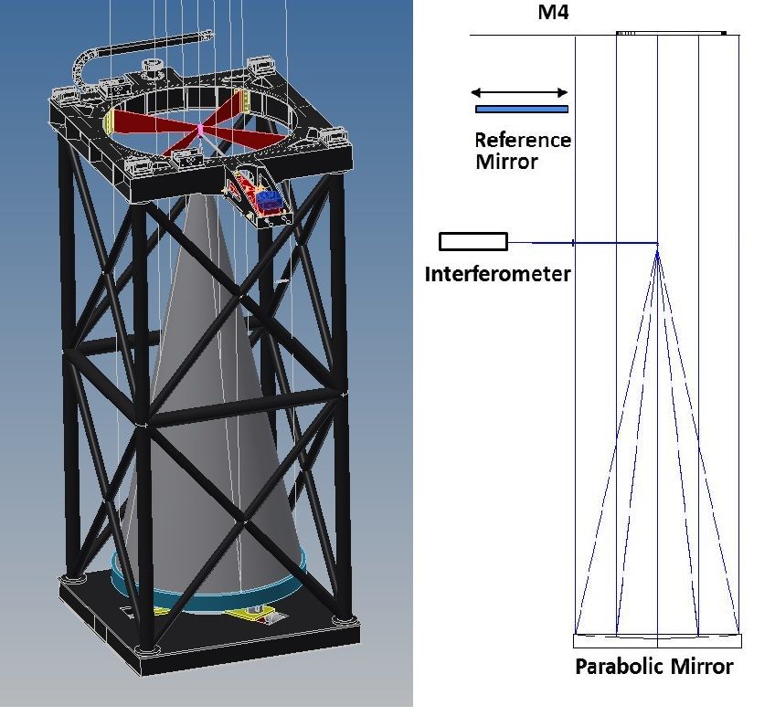
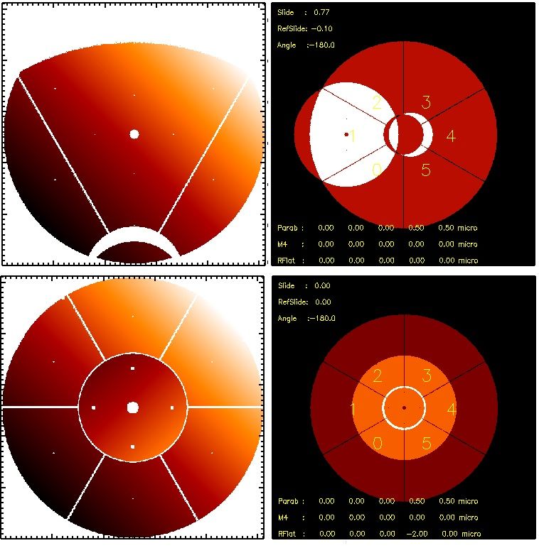
Figure 1. Opto-mechanical drawing of the test tower, with   Figure 2. Mechanical configurations of the OTT with the
the interferometer shining its laser beam toward a relay    parabola looking at (top) a single segment or (bottom) the
system and the parabola. The M4U is not shown here and      central part of all the segments.
is mounted on a larger interface above the OTT.

co-phasing has been extensively addressed during the optical measurements of the M4 prototype M4DP.5 Within
the present scope we will recall the main points of the optical calibration protocol, with the goal to frame the
analysis strategy and the measurement budget.
The preliminary mirror flattening consists in the identification of a set of actuator commands to have the whole
mirror surface within the interferometer capture range. Then, it is possible to collect the mirror modes (modal
and zonal influence functions) required to complete the flattening procedure and the correction of the high order
modes. Alignment aberrations, like piston and tip-tilt, are not corrected at this point. A great attention shall
be paid at this stage to avoid correcting the alignment modes like coma, focus and spherical aberration with the
M4U surface. The calibration of the capacitive sensors, co-located with the actuators, is also performed with a
procedure run separately for each shell. At this step, the presence of neighbour non-active shells may be used
for the correction of vibration noise on the measurement area. At the end of the process, the single shells are
individually flattened. In order to co-phase all the segments, differential tip/tilt and piston is corrected with the
following procedure: the OTT is configured as to image the central part of the M4U (see Fig. 2,bottom panel)
and the local tip/tilt is removed; then, the differential piston is measured with a dedicated Sensor of Phase Lag
(SPL) to remove the lambda ambiguity of the interferometric measurements; in the end the final phasing is
completed with the interferometer, with a goal phasing accuracy of 20 nm RMS wavefront.
The verification of the requirements will be performed after the flattening and phasing of the whole M4 mirror.
The verification measurements include the WFE, both global (full aperture) and local (interactuator pitch),
co-phasing error, slope RMS, local curvature and accuracy of the application of low order Zernike commands.

2.2 Analysis strategy
The strategy for the analysis of the measurement accuracy is described extensively in.6 He we recall that we
considered three main steps:

   • the identification of the measurement types requested for the calibration and performance verification
     routines: more specifically they are differential samplings (for instance to measure with the push-pull
     technique the actuators influence functions) and absolute samplings, to acquire the current mirror WF
     map for the flattening or as a verification measurement;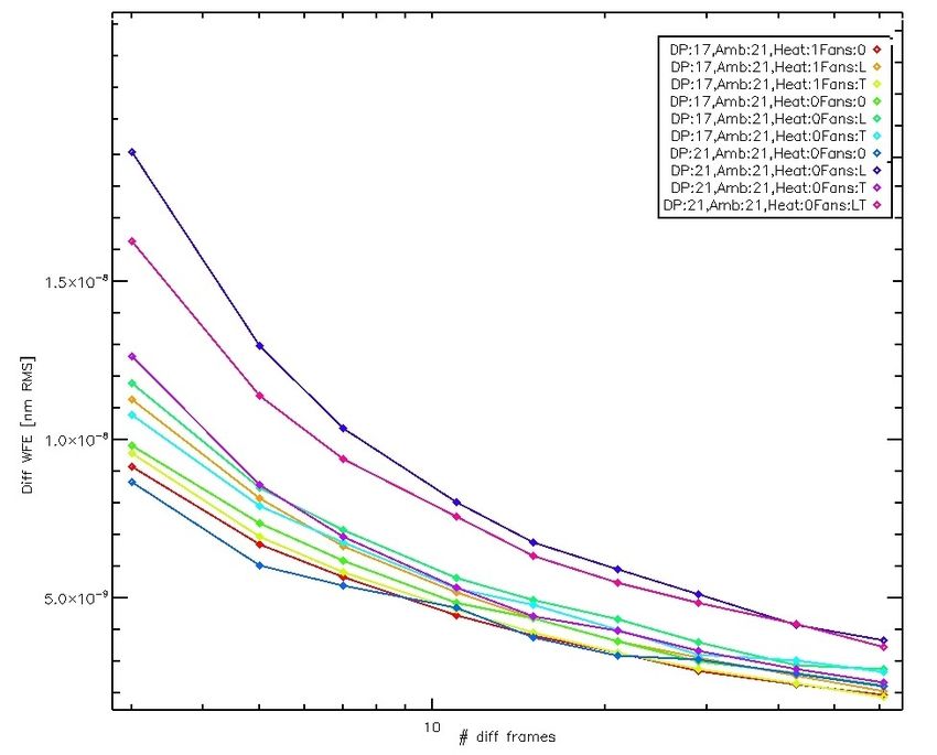
• the identification of the error sources specifically affecting each measurement type, according to the test
     conditions;
   • the noise propagation, including the processing errors, to compute the final measurement budget.

   In the following we describe the error sources and the method to assess their individual contribution. In the
end we take into account the testing protocol and perturb it with the expected noise values, to budget the final
measurement accuracy. Such task, corresponding to an end to end simulation, has been performed with 8s,7 the
simulator of the OTT with M4, specifically designed to assess the calibration protocol.

                      3. EXPECTED MEASUREMENT NOISE SOURCES
3.1 Interferometer CCD noise
We evaluated it by means of a direct measurement on our interferometer on the optical bench: we closed the
cavity with a small flat mirror in front of the exit pupil and collected 2048 frames; then we computed the 1024
differential images to reject the static WF from the cavity; at last we measured for each couple the standard
deviations σW and σs of the WF and of the slope, respectively. √
The frames are statistically uncorrelated, then we can take  = 2 < σ > as an estimator for the measurement
repeatability when collecting a single frame. For the WFE case we obtained  ∼ 2 nm, corresponding to 2 bit
(with a 10 bit resolution the sample the 632 nm phase lag). In terms of slope error, such value corresponds to
0.06 arcsec RMS.
From these value we can calculate the number of frames to average together in order to achieve a target error.
The average of a large number of frames is also requested to reduce the noise input from (e.g.) air convection,
so that we considered the CCD noise already included in the error value from convection.

3.2 Air convection
We considered a procedure for the characterization of the actual convection noise from real data collected in
relevant environments. We took such results, in terms of global WFE (or piston error, slope error, etc) versus
sampling parameters, as the expected OTT convection noise; such values are then scaled according to the
final sampling procedure. The convection noise budget is then converted into a sampling parameters budget.
Operatively, we considered a number of interferometer datasets composed by 1000 frames collected at 25 Hz. They
have been collected during the optical test of the M4DP5 in different environmental conditions, e.g.: ventilation
fans on/off, vertical temperature gradient positive/negative, optical bench open/closed. Such conditions fill the
possible environment parameters space for an optical test environment and are a good representation of a typical
case scenario. We also compared these data with equivalent samplings collected in different laboratories, with
similar conditions, obtaining scalable results.
We will consider in the following two test cases, for absolute or differential acquisition. The allocated convection
budget will be given case by case for each specific requirement.

3.2.1 Absolute measurements
Absolute measurements are collected to sample the current shape of the M4U, for instance during the flattening
process or its verification. The convection noise in absolute measurements is assessed by measuring its coherence
time via the sampling of the noise structure function. The knowledge of the structure function allows the
computation of the number of frames and of the frame rate to obtain a given noise threshold.
The test dataset composed by n frames is analyzed to evaluate the WFE temporal structure function, representing
the convection pattern evolution in time. The goal is to estimate the frame rate and number for a robust
averaging. More details on the computation are given in.6 In Fig. 3 we show a sample of convection structure
functions collected with different environment conditions.
For each plot, the asymptotic value v represents the noise  √ expected after averaging two statistically uncorrelated
realizations. Then the single frame expected noise is v √2. In order to obtain a residual noise v0 , the number
of frames to be average together is computed as n = (v 2/v0 )2 . Such computation is valid if the samples are
statistically uncorrelated, i.e. if convection has fully evolved during the time gap between them. The coherence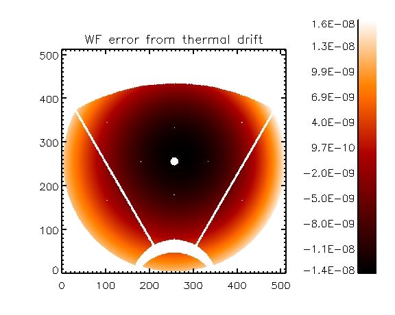
time τ is evaluated by finding the knee of the dataset. Two frames are statistically uncorrelated if they are
collected after a time 2τ .
Once the sampling parameters have been found, we computed the average of n uncorrelated frames and measured
on the averaged image the slope error and the local curvature. From the associated plots, we may estimate the
requested number of frames and the total sampling time to achieve the allocated error budget. The same
procedure may be run to estimated the optimal sampling parameter for differential piston measurements.

3.2.2 Convection noise in differential measurements
Differential sampling is requested to measure the DM response to a given command of amplitude a: for instance
it is used to calibrate e.g. the actuators IF, mirror modes IF, capsens calibration. We refer to these cases
as differential samplings because data are collected with the push-pull technique, i.e. opposite commands are
applied and recorded as WF map difference. The noise from air convection shall be evaluated to estimate the
amplitude a or the integration time to achieve a given SNR. The analysis procedure consists in running the
differential algorithm on a dataset containing a static WF map, i.e. no commands are applied to the DM. We
can then plot the expected differential WFE versus the number of n differences averaged together.
The result for the M4DP case is shown in the picture below. Each plot represents a different environment
condition (as presented above). As expected, the best SNR is achieved with a thermalized optical bench and no
air ventilation. As a comparison, the worst case scenario (i.e. with non-thermalized bench and forced air flux)
leads to a doubled noise level; in this case we need a 4x larger integration to preserve the SNR.
These results are achieved with a frame rate of 25 Hz; faster frame rates yield a better subtraction of correlated
feature and a larger SNR.

Figure 3. Convection structure function on DP test bench   Figure 4. Effect of averaging on differential frames WFE
                                                           (M4DP case)

3.3 Thermal drift
The analysis is based on the opto-mechanical simulation of the OTT. First, we computed (by means of ray
tracing software) the sensitivity matrix for each optical components, in terms of the Zernike aberrations after
perturbing each degree of freedom.
Then we considered the FE model of the OTT and evaluated the thermo-mechanical deformation when subjected
to an unitary temperature variation. We considered both the case of a vertical (and horizontal) thermal gradient
and the case of a unitary thermal step. For each case, the OTT deformation has been re-mapped in terms of
the displacements of the optical components from the interferometer (5 degrees of freedom). The rate of the
temperature variation has been estimated experimentally: we measured the temperature variation of a massive
crane structure placed in a testing facility and exposed to daily thermal cycle. The maximum measurement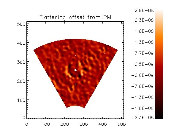
Figure 5. Expected slope error given by air convection ver-   Figure 6. Expected local curvature error given by air con-
sus number of frames averaged.                                vection versus number of frames averaged.

slope (0.65C/hour) may be considered as an upper bound for the temperature variation rate; please note that
the value is however smaller than the rate expected inside the E-ELT dome.
We also evaluated from the FEM the thermal deformation of the parabolic collimator support, which is responsible
for a three-foil shape changing with temperature at a rate of +0.4 nm/C.
At last we computed the total WF map from thermal drift, as the thermal deformation of the parabola plus
the Zernike aberration from mis-alignment induced by the optics displacement. As we know the temperature
variation rate, such result may be indicated both as WFE vs temperature variation and WFE vs measurement
duration. The resulting map is analyzed in terms of global WFE and slope, local curvature and piston error.
For the latter, we considered the piston value as the average phase of the OTT map computed within the optical
mask of one of the M4U segment (see Fig.2), and evaluated its behaviour at changing the relative orientation
segment vs OTT.
Thermal drifts affect absolute measurements only, because of the relatively long time scale of thermal variations
(tens of seconds), compared to the typical frame rate for differential samplings (25 Hz).

Figure 7. Expected WFE due to thermal drift, for a tem-       Figure 8. Mean value over the M4 segment mask of the
perature step of 1C.                                          WFE due to thermal drifts.
3.4 Mechanical vibrations
Mechanical vibrations are responsible for misalignment of the optical components at a relatively high frequency,
thus producing low order aberrations of the WF map (tip-tilt, focus and coma). We considered the FE model
of the OTT and perturbed it with a vibration spectrum acquired in the test facility in daytime (corresponding
to worst case testing conditions) and low-pass filtered according to the dampers transfer function. The dataset
has been analitically applied to the FE model to compute the displacement of the optical components and to
evaluate the corresponding WFE.
The resulting data have been analyzed according to two pipelines: in one case, we computed the WF map after
averaging n frames (simulating absolute samplings); in the other case, we measured the differential WF map at
the interferometer frame rate, to evaluate the differential sampling error. For both cases we measured on the
final maps the total WFE, slope error, local curvature and local piston within the M4U segment mask.

3.5 Processing error
We evaluated the numerical error associated with the data processing algorithms, for two particular cases. The
tilt-detrend function identifies the segment masks within an image and compute their individual tilt values. The
result is used to remove the vibration tilt, measured on the un-active shell, from the active shell, for instance
during push-pull measurements of the mirror influence functions. Alternatively it may be used to evaluate the
differential tilt amongst the segments for the final co-phasing.
The phase-unwrap algorithm is used to correct the interferometer phase ambiguity from the islands in the WF
map, also with the aid of the SPL (see above). A detailed description and validation for both of them is given
in.5
For both cases, the processing error has been evaluated by testing the algorithms on WF maps affected by
thermal drift and vibration noise.

3.6 Optics manufacturing error
A detailed description of the optics manufacturing error is given in.2 The baseline for the testing protocol is
to subtract from the M4U WF map the current OTT cavity, which is given mostly by the shape error of the
PAR. The subtraction error for such static offset is given by two elements: the pixel-to-pixel alignment between
the PAR map and the M4U one and the PAR manufacturing offset. The latter represents the print-through of
the null optics (namely a CGH) used in the optical worskshop to polish the PAR and accounts for the accuracy
error in the calibration shape. The polishing residuals represent on the contrary a precision error. For both
contributions we produced a Montecarlo simulation of polishing/null optics errors (representing the parabola)
and computed the residual after a rigid shift of 2x2 pixel. The residual map was then corrected with the actuator
influence functions to simulate the flattening error. The pupil image relaying optics (RS), which are smaller than
2 inches in diameter, may be calibrated to better than 1 nm WFE RMS and are not considered within this scope.
The calibration of the 100 mm SAI optics will be performed with the same technique and it is budgeted to 3 nm
RMS.

3.7 Retrace error
The retrace error is produced when the interferometer measures the M4U with a large aberration (tilt, power).
Such case applies only during the Zernike test, when large amplitude low order Zernike commands are produced
by the actuators. During the other verification measurements, the optical figuring of the M4U is very low. Under
this assumption, the retrace error is always negligible except for the case of the Zernike test. Within this context,
we modeled with an optical design software the M4 mirror as a Zernike Fringe phase surface, centered on the
M4U axis; we analyzed the difference between the surface applied and the one measured. The computed retrace
error is always lower than 0.3% of the applied Zernike amplitude. It can be therefore neglected also for the case
of the Zernike test.
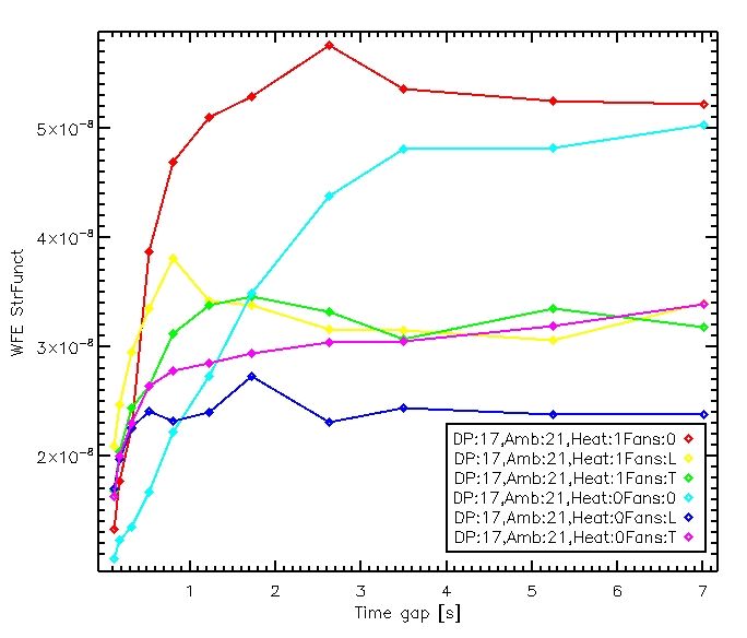
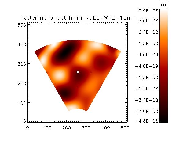
Figure 9. Offset in the actuators flattening command given   Figure 10. Flattening offset from the CGH print-through,
by the parabola polishing precision.                         representing the parabola manufacturing accuracy.

3.8 Zernike fitting error
The measurement of the Zernike alignment modes (focus and coma) in the OTT is performed using the Reference
Flat mirror (RF) as a reference surface. The RF is smaller than the optical surface (0.6 m vs 1.5 m diameter) and
this affects the accuracy of the Zernike modes fitting, in particular in presence of a large tilt offset. We computed
by simulation the relative accuracy of the fitting to evaluate the maximum error expected during alignment.
The test has been performed twice: in a first step, without vibration noise in order to identify the pure fitting
accuracy; in a second step, the test was performed considering also the effects of vibrations noise: in this case
the initial offset includes the Zernike mode to be measured, as it is injected by the optics displacement because
of vibrations. The test took into account different positions of the reference flat. We measured a fit accuracy
better than 3, without correlation with the static offset added. This observation may be explained considering
that the aperture of the RF, although smaller that the optical area, is large enough to allow a correct spatial
sampling of the alignment modes (coma and power), so that the modes fitting is well conditioned. The fitting
accuracy term will be therefore neglected from the budgeting.

3.9 Accuracy of the absolute piston sensor
The OTT is fitted with an absolute piston sensor (SPL) to help solving the interferometer phase ambiguity. Here
we recall that is composed by an illumination system, a camera and a narrow-band, liquid crystal tunable filter;
the working principle has been investigated since many years and a description may be found in.8 The SPL
is requested to verify that the convergence condition is satisfied for the phase ambiguity correction algorithm
(see sec.3.5). The final measurement of the differential piston amongst segments is indeed allocated to the
interferometer. Therefore, the specification for the SPL is to provide a measurement accuracy within just λ/4
across a broad capture range; accordingly, the error budget allocated has the same order of magnitude.
Its measurement error is given by two terms: first, the intrinsic accuracy of the system as-designed can be
evaluated analytically, for instance, the piston accuracy depends on the filter bandwidth (which is known),
leading to a piston uncertainty of 120 nm. The second term is the local differential piston on the sensed area
given by the differential tilt amongst the segments. We budgeted such contribution considering the datasets
collected with the M4DP unit. In that case, the differential tip/tilt between the segments was negligible with
respect to the global WFE (20 nm RMS) so that this term may be neglected for the SPL error budget.

 4. ERRORS PROPAGATION AND VERIFICATION MEASUREMENTS BUDGET
So far we concluded the exercise of the identification of the noise sources within the optical test bench, together
with suitable strategies to assess their contribution. In many cases we converted the error budget into a sampling
parameters budget, such as number of frames, frame rate, total measurement time. We are now able to sum up
the individual error sources into the final measurement accuracy budget. For each of the verification measurement
cases we will consider the applicable noise contributions, scaled according to the proposed procedure and sampling
parameters. Such strategy is presented more in detail in.6

4.1 Mirror flattening accuracy
The flattening process consists in the application of the mirror modes to correct the optical surface. The process
is in close loop with the interferometer, providing at each step the current surface map S to be flattened. The
applicable command is computed by projection of S on to the mirror modes shapes, piled up in the interaction
matrix M . The flattening accuracy is therefore affected by the errors in both S and M ; we will however discard
the last term, because the individual errors in each vector of the M can be negligible (lower than 1 nm RMS).
The errors in the sampling of S comes from measurement noise (precision) and static offset from the optics.
For both cases, the individual contributions may be divided according to their spatial scale: signals within the
actuator spacing (31 mm) are command offset as they may be produced with the actuators and will be observed
regardless the optical system; signals at lower spatial scale affect the verification measurement and will be seen
with the current optical configuration only. We will treat both cases together.
We budget the following contributions:

Convection Air convection affects the flattening command with a random offset in the surface map S. Its
    contribution may be evaluated as discussed in sec.3.2.1, by computing the expected WFE after averaging
    n uncorrelated frames. In the present scope, we fixed the acceptable convection WFE to 5 nm RMS and
    calculated the sampling parameters requested. According to a worst case condition as in Fig.3, the goal
    WFE is obtained by averaging 225 frames collected at a frame rate of 0.5 Hz. Such computation yields
    also the total sampling duration t.
Thermal drifts We computed the thermal deformation occurred during a time step t and considered half of its
    amplitude as the thermal offset for the surface map S. The contribution includes both the misalignment
    induced by thermal bending of the OTT and the surface deformation of the parabola sitting on its 3 pads.
Vibrations We considered the non-averaged misalignment given by vibrations during the time gap t, tip/tilt
    filtered.
Optics manufacturing We computed the optics manufactuing error to flattening as indicated in sec.3.6, as
    the sum of polishing and offset errors. For both cases we considered the print-through on the actuators (as
    the flattening command offset) and the higher orders residual as the verification measurement error.
Processing error We considered the numerical error of the processing algorithms when applied to the expected
    tilt from non averaged vibrations during the time step t.

4.2 Co-phasing accuracy
The co-phasing process is the actuator correction of the rigid modes within the visible area; it consists in the
application of piston, tip and tilt commands produced by the actuators on each segment, in order to make them
laying on the same plane. For the budgeting of the measurement accuracy, we consider a test area of 50 cm
diameter (corresponding to the reference flat mirror aperture) and compute its mean value from the various
error sources. We take such measurement as an estimator of the local piston affecting the M4U measurement of
phasing. The test accuracy error is given by the following contributors:

Convection In Sec.3.2.1 we evaluated the effect of non-averaged convection patterns in terms of mean value
    over a given subaperture depending on number of frames and frame rate. We consider a target noise value
    and identify the sampling parameters to achieve that value.
Thermal drifts We considered the OTT thermal drift during the measurement time and the associated Zernike
    modes, namely power and coma; we then computed the mean value of the alignment aberrations over the
    test area.
Vibrations It affects the piston measurement as the tip-tilt mode measured out of center has a non zero mean
value. We evaluated such contributions from the residual misalignment induced by vibration, as it has
been described in sec.3.4.
Optics manufacturing We computed its contribution as the mean value over the test aperture of the Monte-
carlo realizations of the manufacturing offset as discussed in sec.3.6.
Processing error We considered the mean value over the test aperture of the numerical residues of the pro-
cessing algorithms. We tested them with a WF map given by the non averaged vibration after a time gap
t.
4.3 Surface slope error
The measurement of the surface slope error is performed on the flattened M4U, segment by segment, after
correcting for the OTT alignment. Then the surface map is acquired with the proper sampling parameters and
is re-binned by a factor of 2 in order to reject the pixel-to-pixel noise. The slope error is then measured. We
considered for the verification measurements the following error sources.
Convection From Sec.3.2.1, we have that two un-correlated frames after 2 s. considering a 20 frame averaging
process, we can achieve a slope RMS ¡0.05 arcsec after 40s. So we can set the measurement time to 40s
Thermal drifts, vibrations The contribution is negligible (set to 0.01 arcsec) as the associated signal is mostly
tilt.
Optics manufacturing This is largest contributor, even considering the correction of the interferometric cavity
with parabola WF map. The high spatial scale residues of the subtraction, in facts, are responsible for a
large print-through on the slope signal.
Processing error As for vibration, processing errors are negligible within this context as they are responsible
for tip-tilt only.
4.4 Surface curvature error
The local curvature of the M4U optical surface after the flattening processing is requested to be larger than
80 km−1 , in order to prevent the scalloping effect of the primary mirror segments. The spatial scale of the
requirement is 80 mm, corresponding indeed to the projected size of the M1 segments on the M4U. We computed
the minimum local curvature (maximum error) for each noise sources and the analysis is presented below.
Convection We can consider a time for a single un-correlated frame of 2s. After that, according to 12.1.3.2,
considering a 30 frame averaging process, we can achieve curvature radius ¡1/1000 Km-1 after 60s. So we
can set the measurement time to 60s.
Thermal drifts For the measurement time considered, the contribution is negligible.
Vibrations For the measurement time considered, the contribution is negligible.
Optics manufacturing The simulated manufacturing residue maps have been analyzed to compute the local
curvature, showing up that the optics offset is the major contribution to this term, in particular, the
print-through of the CGH.
Processing error The analysis showed that the contribution in terms of local curvature is negligible.4.5 Surface error at the high spatial scales
After flattening and co-phasing the M4U segments, the measurement of the high spatial frequency is performed
with a secondary interferometer with a 100 mm measuring beam. The goal of such additional measurement is
to certify the WFE at the inter actuator scale, affected by the polishing of the shells. The measured area moves
across the M4U to sample a statistically relevant number of subapertures. We recall here that the flattening
procedure is performed with the LAI setup, while the verification measurement is done in SAI mode. The
advantage of such a strategy is to reject (at least in part) from the verification measurements the high spatial
frequency of the parabola, which is in double pass in the OTT. When switching from LAI to SAI, the PAR print-
through is impressed on the M4U after the flattening procedure and will therefore give a WF signal measured
on SAI. As a second point, the SAI system is insensitive to local tip-tilt at the spatial scale of 100 mm, as it
is realigned at any measurement position. As a consequence, the SAI cannot measure M4U flattening offsets
in the form of local tip-tilt on 100 mm patches and such contribution from LAI shall be therefore budgeted as
well. We considered therefore the high frequency errors for both optical systems, namely: flattening offset at the
interactuator scale from the LAI manufacturing; WF offset in the measurement from the SAI manufacturing;
thermal drifts, vibrations and convections. Additionally, we needed to budget also the tip-tilt errors at the
measurement scale (100 mm) as this contribution is removed with the SAI alignment.
Convection We set a 160 s of measurement time (80 measurements sampled at 0.5 Hz) and evaluated the
residual convection noise on the 100 mm measurement patch, both in terms of tip-tilt offset and WFE at
the interactuator scale.
Thermal drifts, vibrations We considered the higher orders beyond tip-tilt due to alignment of M4U and
SAI cavity during the measurement time. The computed value is lower than 1 nm WFE so it is set to be
conservative to 1 nm.
Optics manufacturing The flattening print-through at the inter-actuator scale has been evaluated on the
simulated manufacturing residuals. The contribution is negligible for the manufacturing accuracy (CGH
term) and approximately 5 nm RMS for the plishing precision. The local tip-tilt at the measurement spatial
scale is on the opposite dominated by the CGH term, accounting for 4 nm RMS. Finally, the contribution
of the SAI optics (which can be calibrated at high accuracy on the test bed) have been budgeted to 3 nm
RMS.
Processing error Has been considered negligible as they account for tip-tilt residuals only.
4.6 Low order Zernike command error
The test procedure consists in the fitting of the desired Zernike shape onto each individual segment, then the
command is applied and measured in push-pull. The main errors sources are described in the following:
Convection The measurement is done with a differential sampling, so that the considerations in sec.3.2.2 may
be applied. The convection noise affects primarily the IF sampling, requested to fit the Zernike modes. It
has been therefore considered as a noise input for the processing, described below. The sampling parameters
are set as 25 frames in 1 s.
Thermal drifts, vibrations We simulated the time evolution of both thermal drifts and vibrations, sampled
with differential acquisition at 25 Hz frame rate. We computed the residual noise as the average WFE of
the differential frames.
Optics manufacturing This error source is not applicable as the differential sampling rejects the static offset.
Processing error the computation of the Zernike command is performed by projecting the wanted shape onto
the actuators IF. The noise of the IF measurement is propagated to the final command, thus adding to
the shape achieved a random error. The SNR for the low order modes is tipically very good (SNR > 50),
however in order to achieve a fitting error matching the REQ, the command should include the high ordermodes as well. We considered three reference convection noise values for the IF measurements: 5 nm, 10
nm, 25 nm. Such values represents typical results obtained with the differential sampling (see 12.2.3). We
computed the wanted Zernike commands and took the resulting shapes as fitting error references. The
we re-computed the Zernike commands after injecting in the IF dataset a random noise with the given
amplitudes. We then computed the difference of the shapes obtained wrt the reference ones. Thanks to this
procedure, the noise of the IF is propagated throughout the command computation procedure, including
the inversion of the interaction matrix.
Retrace error The discussion on this error source is fully described in Sec. 3.7.
4.7 Total error budget
The final error budget table is given below, where we report the individual contributions for all the cases dis-
cussed. The values are given (when applicable) as WFE For the curvature error, the total value has been
computed by summing up the individual curvature map and the measuring the resulting shape.
Flattening Phasing Slope err. Curv. err. High sp. freq. Zernike test
nm nm arcsec km nm nm
Convection 5 10 0.07 1/1000 5 10
Thermal drifts 2 2 0.01 negl. 1 1
Vibrations 1 1 0.01 n.a. 1 1
Opt. accuracy 7 5 0.28 1/106 7 n.a.
Opt. precision 15 n.a. (tot) (tot) (tot) n.a.
Processing err. 1 3 0.01 n.a. negl. < 1% comm.
Total 18 12 0.29 1/96 9 11 nm, 1.1% comm.
5. LESSON LEARNED AND REMARKS
At the end of the analysis process, we find that the error budget is within the requirements for all the measure-
ment cases considered. We notices however some critical points that shall be carefully addressed to reduce the
associated risks.
The OTT optics foot-print is a remarkable offset for the budget, in particular the nulling system used during the
manufacturing of the parabola. The measurement of its low-mid spatial scales could be in principle performed
on the OTT itself without a null optics, illuminating the mirror from its focus and reflecting back the collimated
output with the M4 surface. The foot-print of the latter may be removed with a robust spatial averaging, i.e.
by sliding and rotating the OTT structure and imaging many patches of M4. The reference flat may be used to
cross-check the results, at least over patches of 60 cm diameter.
The thermal drifts have been computed starting from a temperature variation of 0.65C/hour; we considered, as
a risk mitigation strategy, to wrap the OTT with insulation sheets to keep the internal temperature stable and
moreover to suppress air convection during high frequency, differential samplings. Also, the location of the OTT
during the calibration procedure shall be selected considering the diurnal and seasonal temperature variation of
the building. Ventilation fans will be installed inside the tower to break the static air bubbles and improve the
accuracy of absolute interferometric measurements (see also Sec.3.2.1).
The SPL measurement of the initial piston between adjacent segments is affected by the residual differential tilt,
so that the phasing procedure will be performed in two steps: adjustment on the differential alignment and then
phasing. Care shall be taken in the management of the SPL small sensing areas, so as to avoid spurious signals
from local bumpiness or imperfect bavels.
As a last remark, the alignment focus from the parabola shall be accurately nulled to avoid its print-though
in the actuator flattening command. This would inject a higher order spatial scale waviness on the shells as a
consequence of the stress release of the glass, with a significant loss in terms of residual WFE.
We prepared a laboratory set-up to further assess some measurement cases. We named it microOTT and its final
goal is to re-create a representative version of some equipment in the OTT and perform validation measurements
to identify and possibly solve the related issues.6. CONCLUSION
We presented a bottom-up approach for the measurement error budgeting of the optical calibration of M4,
the E-ELT adaptive mirror. We considered the system requirements and the breakdown of the interferometric
measurements requested for the verification. We identified the error sources associated with each measurement
and computed their contribution. For the cases of environmental noise (.e.g. air convection or thermal drifts) we
converted the error budget into a sampling parameters budget, such as frame rate, number of averaged frames,
in order to meet the desired accuracy.
The error budget is within specifications for all the test cases: the largest contributor to WFE is the collimation
optics so that an accurate measurement of its shape shall be requested. We identified the most challenging issues
and set up a laboratory experimentation to validate the solutions proposed. The optical verification of the OTT
will start at the beginning of 2019 and the calibration of the M4 is scheduled for 2023.
REFERENCES
[1] R. Biasi, M. Manetti, M. Andrighettoni, G. Angerer, D. Pescoller, C. Patauner, D. Gallieni, M. Tintori,
M. Mantegazza, P. Fumi, P. Lazzarini, R. Briguglio, M. Xompero, G. Pariani, A. Riccardi, E. Vernet,
L. Pettazzi, P. Lilley, and M. Cayrel, “E-ELT M4 adaptive unit final design and construction: a progress
report,” in Adaptive Optics Systems V, Proc. of SPIE 9909, p. 99097Y, July 2016.
[2] G. Pariani, R. Briguglio, M. Xompero, and al., “Optical calibration of the ELT: design, alignment and
verification of the interferometric test tower,” in Proceedings of the Fifth AO4ELT Conference, July 2017.
[3] A. Riccardi, M. Xompero, R. Briguglio, F. Quirós-Pacheco, L. Busoni, L. Fini, A. Puglisi, S. Esposito,
C. Arcidiacono, E. Pinna, P. Ranfagni, P. Salinari, G. Brusa, R. Demers, R. Biasi, and D. Gallieni, “The
adaptive secondary mirror for the Large Binocular Telescope: optical acceptance test and preliminary on-sky
commissioning results,” in Adaptive Optics Systems II, Proc. of SPIE 7736, p. 77362C, July 2010.
[4] R. Briguglio, M. Xompero, A. Riccardi, M. Andrighettoni, D. Pescoller, R. Biasi, D. Gallieni, E. Vernet,
J. Kolb, R. Arsenault, and P.-Y. Madec, “Optical calibration and test of the VLT Deformable Secondary
Mirror,” in Proceedings of the Third AO4ELT Conference, S. Esposito and L. Fini, eds., p. 105, Dec. 2013.
[5] R. Briguglio, M. Xompero, A. Riccardi, and al., “Optical calibration of the M4 prototype toward the final
unit,” in Proceedings of the Fourth AO4ELT Conference, Nov. 2015.
[6] M. Xompero, R. Briguglio, G. Pariani, and al., “Optical calibration of the ELT: strategy for the optical
measurement error estimation,” in Proceedings of the Fifth AO4ELT Conference, July 2017.
[7] R. Briguglio, G. Pariani, M. Xompero, A. Riccardi, M. Tintori, P. Lazzarini, and P. Spanò, “8s, a numerical
simulator of the challenging optical calibration of the E-ELT adaptive mirror M4,” in Adaptive Optics Systems
V, Proc. of SPIE 9909, p. 99097A, July 2016.
[8] M. Bonaglia, E. Pinna, F. Quiros-Pacheco, A. Puglisi, and S. Esposito, “Large capture range cophasing
with the Liquid Crystal Tunable Filter,” in Ground-based and Airborne Telescopes II, Proc. of SPIE 7012,
p. 70123C, July 2008.You can also read