Chemistry at the Nanoscale - When Every Reaction is a Discrete Event
←
→
Page content transcription
If your browser does not render page correctly, please read the page content below
GENERAL ARTICLE

                       Chemistry at the Nanoscale
                      When Every Reaction is a Discrete Event

                           Ashwin B R Kumar and Ram Ramaswamy

Traditionally the kinetics of a chemical reaction has been stud-
ied as a set of coupled ordinary differential equations. The
law of mass action, a tried and tested principle for reactions
involving macroscopic quantities of reactants, gives rise to de-
terministic equations in which the variables are species con-
centrations. In recent years, though, as smaller and smaller
systems – such as an individual biological cell, say – can be           Ashwin B R Kumar is a
studied quantitatively, the importance of molecular discrete-           graduate student in the
                                                                       Biophysics, Structural and
ness in chemical reactions has increasingly been realized. This          Computational Biology
is particularly true when the system is far from the ‘thermo-         Program, School of Medicine
dynamic limit’ when the numbers of all reacting molecular              and Dentistry, University of
species involved are several orders of magnitude smaller than           Rochester, New York. His
                                                                         research interests are in
Avogadro’s number. In such situations, each reaction has to               studying the structure,
be treated as a probabilistic ‘event’ that occurs by chance           function, interaction and the
when the appropriate reactants collide. Explicitly account-           chemistry of biomolecules as
ing for such processes has led to the development of sophisti-         well as their assemblies and
                                                                                networks.
cated statistical methods for simulation of chemical reactions,
particularly those occurring at the cellular and sub-cellular
level. In this article, we describe this approach, the so-called
stochastic simulation algorithm, and discuss applications to
study the dynamics of model regulatory networks.
                                                                      Ram Ramaswamy teaches in
                                                                        the Schools of Physical
                                                                          Sciences (SPS) and
1. Introduction
                                                                           Computational and
                                                                      Integrative Sciences (SCIS) at
The subject of chemical kinetics essentially relates to the study
                                                                      Jawaharlal Nehru University,
of the progression of chemical reactions and the rates of transfor-     New Delhi. His research
mation of chemical species from reactants to products [1, 2]. The     focuses on nonlinear science
discipline traces its origins to 1850 when the rate of inversion        as well as computational
                                                                            systems biology.
of sucrose into glucose and fructose was modelled by the Ger-
man chemist Ludwig Wilhelmy who used an ordinary differential

RESONANCE | January 2018                                                                              23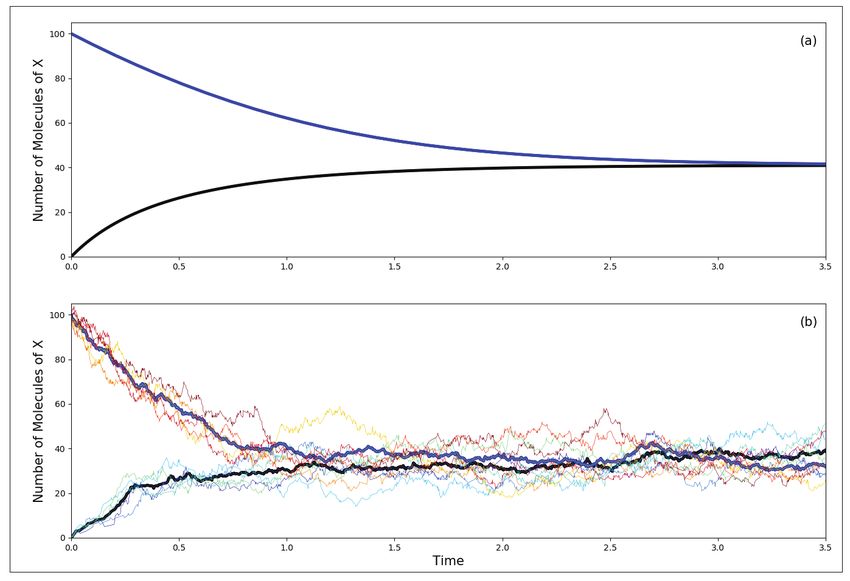
GENERAL ARTICLE

Keywords                              equation (ODE) to describe the process mathematically. Shortly
Chemical    kinetics,   stochastic    thereafter, Guldberg and Waage proposed the law of mass action,
chemical    kinetics,   Gillespie’s
                                      after which the subject developed rapidly, with important contri-
stochastic simulation algorithm,
synthetic gene oscillators.           butions coming from van’t Hoff, Arrhenius and Ostwald among
                                      others. The importance of understanding how chemical reactions
                                      occurred, and what factors affected their rates or efficiency has
                                      always been a matter of great practical importance. The major
                                      advances of the late 1800s were quickly recognised with Nobel
                                      Prizes, the very first in 1901 going to van’t Hoff for his work on
                                      the development of chemical kinetics, chemical dynamics, and
                                      on the concept of osmotic pressure. Arrhenius’ derivation of the
                                      eponymous rate equation led to his Prize in 1903, and in 1909 to
                                      Ostwald, for several contributions to physical chemistry that in-
                                      cluded the principle of independence of chemical reactions, and
                                      the study of catalysis and chemical kinetics.
                                      The classical approach to study the kinetics of a chemical reac-
                                      tion is to use one or more ODEs to analyse the time evolution
                                      of concentrations of the various chemical species involved. This
                                      approach, although recognising that chemical reactions are binary
                                      events on the molecular scale, encapsulates the details of all inter-
                                      actions into effective rates that apply when the chemical species
   The classical approach             are abundant. The concept of the order of a reaction and the de-
 to study the kinetics of a           pendence of the rate on the stoichiometry of the reaction implies
    chemical reaction is to
                                      that the method for modelling chemical reactions is in terms of
use one or more ODEs to
           analyse the time           continuous variables that obey deterministic equations of motion.
               evolution of           However, this approach is inadequate when the populations of
     concentrations of the
various chemical species              the chemical species are very low. For instance, in a typical bi-
involved. This approach,              ological cell, the total number of molecules ranges from 109 (for
     although recognising             bacteria) to 1013 (for a eukaryotic cell) or so. The number of
   that chemical reactions
                                      molecules of biological interest is much smaller than this, rang-
  are binary events on the
           molecular scale,           ing from one (for DNA) to a few hundred RNA to a few thousand
  encapsulates the details            proteins. Although the effective concentrations are in the nano-
    of all interactions into          or sub-nanomolar range, advances in experimental techniques to
 effective rates that apply
                                      study single molecules have made it possible to investigate the
        when the chemical
     species are abundant.            dynamics (and hence also the kinetics) at this scale. In such sys-
                                      tems, a classical kinetics approach cannot accurately predict the

24                                                                                RESONANCE | January 2018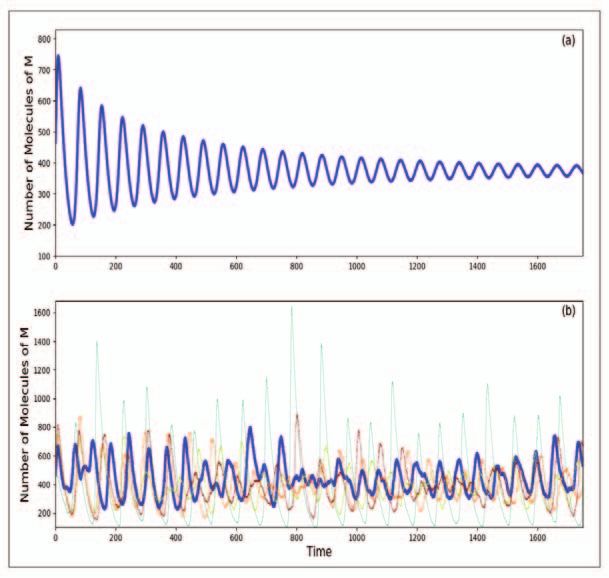
GENERAL ARTICLE

behaviour; most of the assumptions underlying the law of mass         At the microscopic level,
action and kinetic theory are not valid.                              chemical reactions occur
                                                                      when two molecules
At the microscopic level, chemical reactions occur when two           come close enough, in
molecules come close enough, in the proper relative orientations,     the proper relative
                                                                      orientations, and with
and with the appropriate relative energies and angular momen-
                                                                      the appropriate relative
tum to interact, namely, either to make new chemical bonds or         energies and angular
to break existing ones and sometimes both. The reaction mech-         momentum to interact.
anism for any given reaction is a way of interpreting this state-
ment on a microscopic basis, while the macroscopic rate laws are
a means of rationalising experimental results. Clearly, both these
descriptions mask a wealth of detail since at the microscopic level
molecules scatter off each other with specific energy and angular
momentum, and the probability of reaction is related to the scat-
tering cross section. Such quantities cannot be computed with
quantitative accuracy for any but the most elementary reactions:
the calculations are straightforward but tedious, and essential in-
puts such as interaction potentials are not known to sufficient ac-
curacy.
An intermediate – mesoscopic – approach recognises the fact that
when the number of molecules is not very large, a probabilistic
approach can be used. Thus, the collision of two reactant species
can be thought of as a random event that depends on the number
of each of them and the volume of the container. Each such colli-
sion leads to a reaction with some probability, and each reaction
changes the number of each species in a discrete fashion. When
there are several possible reactions, depending on the number and
types of species, these are taken to be concurrent random pro-
cesses; the randomness and discreteness become very significant
when the numbers are small and far from the so-called thermody-
namic limit. The stochastic nature of chemical reactions in such
situations becomes significant since noise plays a major role in
the evolution and response of such systems.
Stochastic approaches to the study of chemical reactions can be
traced back to the early work of Kramers [3] and Delbrück [4],
who modelled the stochastic dynamics of an autocatalytic reac-
tion, followed by numerous other studies that have been summa-

RESONANCE | January 2018                                                                     25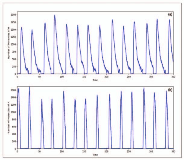
GENERAL ARTICLE

           The stochastic   rized in the very influential review article by McQuarrie in 1967
     simulation algorithm   [5]. The practical implementation of this methodology was enun-
       (SSA) proposed by
                            ciated in a very lucid article by Gillespie [6] a decade later. To-
 Gillespie is widely used
to simulate the dynamics    day, his formulation of the stochastic simulation algorithm (SSA)
          of chemical and   is widely used to simulate the dynamics of chemical and bio-
 biochemical reactions in   chemical reactions in nanoscale environments. In addition to the
nanoscale environments.     already noted applications to cellular and subcellular processes,
                            similar considerations will also apply to chemical reactions oc-
                            curring on (say) dust grains in interstellar space where tempera-
                            tures and densities are very low, and the probability of molecular
                            encounters are consequently very small.

                            2. Stochastic Simulation Algorithm

                            The law of mass action that is taught early in all chemical kinetics
                            courses states that the rate of a chemical reaction is proportional
                            to the product of the concentrations of the reacting substances,
                            with each concentration raised a power that is the stoichiomet-
                            ric coefficient in the corresponding chemical equation. The fact
                            that this is only true in limited cases becomes clear in even sim-
                            ple examples such as the reaction between hydrogen and iodine
                            chloride, with the formation of iodine and hydrogen chloride [2],

                                                 H2 + 2ICl → I2 + 2HCl

                            for which one would write (incorrectly, as it turns out) the rate as
                            proportional to:
                                                      [H2 ][ICl]2
                            (where [X] represents the concentration of X), which is a third-
                            order reaction. Experimentally though, the reaction is seen to
                            be of second-order, consistent with the microscopic description
                            comprising two consecutive reactions,

                                  H2 + ICl → HI + HCl      and HI + ICl → I2 + 2HCl

                            The first reaction is slow while the second is much more rapid.
                            Thus, the rate is actually proportional to [H2 ][ICl], making it ef-
                            fectively a reaction of second-order.

26                                                                     RESONANCE | January 2018
GENERAL ARTICLE
The Gillespie approach is to treat such consecutive or concurrent
reactions within a general framework. Say there are N chemical
species, X1 , X2 , X3 , . . . , XN that can participate in M distinct
reactions, each of which has the form:
Reactants → Products
The ‘Products’ on the right-hand side can be one or more of the
molecules being considered here, namely from within the set of
the Xi ’s, in which case these can subsequently participate in one
or the other of the M reactions that are possible. The products
can also be other molecules that do not participate in the reactions
being considered, in which case these are denoted by ∅. Similarly,
the reactants can be from the set of the Xi ’s or can include other
molecules, as will be made clear in the examples discussed below.
The configuration at any instant of time, namely the numbers of
the different molecules that are present is denoted by the inte-
gers n1 , n2 , . . . , nN . Each of the reactions is treated as a Poisson
random process that occurs at a specific rate that depends on the
propensity of the reaction. The propensity for each of the reac-
tions depends on the configuration (see Box 1 for details of how
these are computed). The essential component of the Gillespie
algorithm is a recipe for determining which of the M different
reactions will actually occur, and more importantly, when it will
occur. At each step, therefore, one determines the time of the next
reaction by generating an exponentially distributed random num-
ber which is based on the overall rate of any reaction occurring,
given the specific configuration and the resulting propensities.
Therefore, given a configuration at a point in time, one can find
out when the next reaction will occur as well as which reaction
it will be. One simultaneously advances the internal time and The essential component
changes the configuration, depending on the stoichiometry of the of the Gillespie
algorithm is a recipe for
reaction that occurs. It is important to note that the direct ver-
determining which of the
sion of the SSA is statistically exact. Being simple to understand, M different reactions will
it is also easy to implement although it can become computa- actually occur, and more
tionally slow and expensive when the complexity of the system importantly, when it will
under consideration increases. At present, there are a number of occur.
RESONANCE | January 2018 27GENERAL ARTICLE
For a proper ‘systems improvements to the basic algorithm and alternative approaches
level’ understanding of that have made stochastic simulation methods considerably faster
biological processes, a
[7].
computational approach
is useful owing to the
inherent complexity of 3. Modelling Stochastic Dynamics
the various interacting
processes that are
involved in even the
Current experimental techniques allow for the measurement of
simplest cases. the rates of many elementary reactions. For a proper ‘systems
level’ understanding of biological processes, however, a compu-
tational approach is useful owing to the inherent complexity of
the various interacting processes that are involved in even the
simplest cases. In conjunction with experiments, computational
modelling can, therefore, provide some insight into the system
dynamics.
Implementation of SSA is best discussed in the context of sim-
ple model systems for which the dynamics can be analysed in
detail. One such set of coupled autocatalytic reactions that was
proposed by Schlögl [8] consists of four reactions R1−4 involving
three species denoted as A, B, and X:
c1
R1 : A + 2X −→ 3X
c2
R2 : 3X −→ A + 2X
c3
R3 : B −→ X
c4
R4 : X −→ B
where the rates of the equations are indicated by the ci ’s. The pop-
ulations of A and B are taken to remain constant and much larger
than that of the species of interest, namely X. For this dynamics,
it is straightforward to obtain the kinetic equation:
dx
= c1 ax2 − c2 x3 + c3 b − c4 x,
dt
where a, b, and x are the concentrations of A, B, and X respec-
tively. Although nonlinear, the above equation can be easily solved
for specific values of the rate constants ci ’s and a and b; typical
results are shown in Figure 1.
28 RESONANCE | January 2018GENERAL ARTICLE
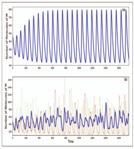
Figure 1. Panel (a) shows
the temporal behaviour of X
obtained by solving the ki-
netic equation for parameter
values: a = b = 105 , and
c1 = 3·10−7 , c2 = 10−4 , c3
= 10−3 , and c4 = 3.5 for two
different values of the initial
concentration of X which in
steady-state reaches a value
of 40. Panel (b) shows
the results from a stochastic
simulation. The bold lines
in (b) are averages of several
independent runs carried out
with similar initial condi-
tions as in (a). As can be
seen, there is clearly a simi-
larity in the average stochas-
tic behaviour and the results
of the deterministic simula-
tion, the agreement getting
better as the system size is
increased.
The key contrast between stochastic and deterministic modelling
of a reaction system can be seen in this example. As we can
see from the simulation of the Schlögl reactions shown in Fig-
ure 1(b), each stochastic run gives a different trajectory for the
time evolution of the reaction (each thin line represents a spe-
cific run), whereas in the deterministic modelling approach every
simulation will give the same trajectory for the specified initial
conditions. One, therefore, takes an average of several stochas-
tic simulations (the bold lines in Figure 1(b)) in order to make a
proper comparison with the kinetic simulations in Figure 1(a).
RESONANCE | January 2018 29GENERAL ARTICLE
3.1 Dynamics of Biological Systems
Periodic variations in the This approach to chemical kinetics is particularly suited to the
concentrations of study of biological systems since, as pointed out earlier, many of
specific biomolecules
the reactant species occur in small numbers within cells. Indeed,
play an extremely
important role in one of the earliest applications was to the kinetics of the genetic
regulation of the switch in the λ-phage system [9]. By now, there are numerous ex-
biological processes they periments that have directly shown the influence of stochasticity
are invloved in, a feature in biochemical reactions in both prokaryotic and eukaryotic cells.
that has been studied
extensively in naturally Here we focus on oscillatory behaviour. The maintenance of
occurring systems as rhythms is extremely important in biology – many biological
well as in synthetic
oscillators. ‘clocks’ play a crucial role in the functioning of organisms. Os-
cillations in biology are known to range from timescales of mil-
liseconds as in neuronal processes, to seconds as in calcium os-
cillations or cardiac rhythms, to circadian clocks that have a pe-
riodicity of about one day or 24 hours. Longer periodicities are
also known, such as ovarian cycles that last a month, and ecolog-
ical cycles that have timescales of years. All such rhythms are
dominated by fluctuations. In fact, to recognise and celebrate the
importance of the research on biological clocks, the Nobel Prize
in Physiology or Medicine for the year 2017 was awarded to Hall,
Rosbash and Young for their research on molecular mechanisms
1 For interesting information on of the circadian rhythm1 .
‘circadian rhythms’, see Series
Article by K M Vaze, V K The area of systems biology, which aims to study the dynamics
Sharma and K L Nikhil, Reso- and behaviour of a network of biological reactions is currently
nance, Vol.18, No.7, 9 and 11, of great interest. In most biological systems, there are several
2013; Vol.19, No.2, 2014.
reacting biochemical species, and an interesting aspect of the dy-
namics in such networks is sustained oscillation in the concentra-
tion of key molecules. Such periodic variations play an extremely
important role in regulation, a feature that has been studied ex-
tensively in naturally occurring systems as well as in synthetic
oscillators.
An early example of a synthetic gene oscillator model with oscil-
lations was proposed by Goodwin [10] in which a gene produces
a protein that represses its own expression as shown in Figure 2.
30 RESONANCE | January 2018GENERAL ARTICLE
This model consists of the following six reactions:
c1
R1 : D −→ D + M
c2
R2 : M −→ M + P1
c3
R3 : P1 −→ P2
c4
R4 : M −→ ∅
c5
R5 : P1 −→ ∅
c6
R6 : P2 −→ ∅
that involve four molecular species. D and M correspond re-
spectively to the promoter region on the DNA and the messenger
RNA. P1 is the protein product from M and P2 is its transcrip-
tional repressor form. The model has been used extensively for
studying the dynamics of enzyme catalysis, transcriptional gene
regulation, and multi-site protein phosphorylation processes.
The kinetic equations derived by Goodwin [10, 11] are:
dM 1
= − αM ,
dt 1 + Pn2
dP1
= M − βP1 ,
dt
dP2
= P1 − γP2 ,
dt
where M, P1 , and P2 are the concentrations of M, P1 , and P2 re-
spectively. The negative feedback due to the inhibition caused by
P2 on the production of M is described by a Hill function, with
Figure 2. Biochemical
network for the Goodwin
model. D denotes the pro-
moter region on the DNA, M
denotes the mRNA, P1 is the
protein product, while P2 is
the transcriptional repressor
form of P1 .
RESONANCE | January 2018 31GENERAL ARTICLE
Figure 3. Dynamics of M
in the Goodwin model for
n=10. The other parame-
ters have the values c2 = c3
= 0.075 min, c4 = c5 =
c6 = 0.0375 min−1 and s
= 300. The deterministic
dynamics is shown in (a)
above and the correspond-
ing stochastic dynamics is
shown in (b) below. While
the deterministic dynamics
at these values of the param-
eters clearly leads to damped
oscillations in the stochastic
version, the motion is not as
clearly damped. Such a dif-
ference between determin-
istic and stochastic simula-
tions highlights the need for
stochastic simulations when
the systems are small.
the coefficient n being treated as a parameter. It is known [11] that
below n = 8 the dynamics is damped, while for larger n there can
be limit cycle oscillations for suitable values of other parameters.
Setting up the SSA for this system can be done in a straightfor-
ward manner, treating the negative inhibition as a modification of
the basic rate c1 . When the system size s is included in the for-
malism it can be shown that this changes the effective values of
the propensity as c1 = 3sK n /4(K n + Pn2 ) molecules min−1 , where
K ≡ s molecules.
As can be seen in Figures 3 and 4, there are significant similarities
as well as differences between the deterministic dynamics and
the stochastic dynamics even when describing the same system,
emphasising the need to use the appropriate formalism depending
on the situation being modelled.
32 RESONANCE | January 2018GENERAL ARTICLE
Figure 4. Dynamics of
M in the Goodwin model
for n=15; other parameters
as in Figure 3. The deter-
ministic dynamics is shown
in (a) above and the corre-
sponding stochastic dynam-
ics is shown in (b) below.
The deterministic dynamics
at these values of the param-
eters clearly leads to a limit
cycle with sustained oscilla-
tions. In the stochastic ver-
sion, however, the dynam-
ics while oscillatory, is not
strictly periodic. This differ-
ence reduces as the volume
increases.
Another simple model of biological oscillations was proposed by
Vilar, Kueh, Barkai, and Leibler [12] (VKBL). The genetic net-
work of this model, shown diagrammatically in Figure 5 is some-
what more complex than the simple feedback loop proposed by
Goodwin and consists of two genes, an activator A and a repressor
R in a negative feedback loop. The activator A promotes its own
transcription as well as that of R by binding to the correspond-
ing promoters. The repressor R acts negatively by sequestering
A through the formation of an activator-repressor complex. This
combination of positive and negative feedbacks yield sustained
oscillations.
There are sixteen different processes that need to be considered
in the VKBL network, and these give the following ‘chemical’
RESONANCE | January 2018 33GENERAL ARTICLE
Figure 5. Biochemical net-
work of the VKBL model
[12]. DA and DR denotes
the promoter regions on the
DNA without the activator
A bound for gene A or R;
DA and DR denotes the pro-
moter regions on the DNA
with the activator A bound
for gene A or R; MA and
MR denotes the mRNA for
A and R, while C represents
the complex formed by A
and R.
reactions:
c1 c9
R1 : DA + A −→ DA R9 : A + R −→ C
c2 c10
R2 : DA −→ DA + A R10 : A −→ ∅
c3 c11
R3 : DR + A −→ DR R11 : DR −→ DR + MR
c4 c12
R4 : DR −→ DR + A R12 : DR −→ DR + MR
c5 c13
R5 : DA −→ DA + MA R13 : MR −→ ∅
c6 c14
R6 : DA −→ DA + MA R14 : MR −→ MR + R
c7 c15
R7 : MA −→ ∅ R15 : C −→ R
c8 c16
R8 : MA −→ MA + A R16 : R −→ ∅
Application of the stochastic simulation algorithm is fairly straight-
forward, given the above equations. The temporal variations in R
and A obtained through stochastic simulations are shown in Fig-
ure 6. The reaction rates (see the caption of Figure 6 for their
values) have been measured or estimated and putting all these to-
gether, one can clearly see that the concentrations of R and A vary
in an oscillatory manner, with a period of about 24 hours.
34 RESONANCE | January 2018GENERAL ARTICLE
Figure 6. Results from the
stochastic simulations of the
VKBL model showing the
variation of repressor in (a)
and protein A in (b) as a
function of time (in hours).
The circadian nature of the
oscillations is evident. In
these simulations we have
used the parameter values c1
= 1 mol−1 h−1 ; c2 = 50 h−1 ;
c3 = 1 mol−1 h−1 ; c4 = 100
h−1 ; c5 = 500 h−1 ; c6 = 50
h−1 ; c7 = 10 h−1 ; c8 = 50
h−1 ; c9 = 2 mol−1 h−1 ; c10
= 1 h−1 ; c11 = 50 h−1 ; c12 =
0.01 h−1 ; c13 = 0.5 h−1 ; c14
= 5 h−1 ; c15 = 1 h−1 ; c16 =
0.2 h−1 . Some of these reac-
tion constants have been ad-
justed so as to give the near
4. Summary 24 hour periodicity. The ini-
tial conditions are DA = DR
Realistic simulations of biological systems have become possi-
= 1 mol, DA = DR = MA
ble since many of the basic rates – the cμ ’s for many elemen- =MR = A=R=C=0.
tary processes – can now be measured, making the overall system
amenable to modelling. This methodology has greatly enhanced
our understanding of the existing genetic networks in biological
cells and also helped in the design of new ‘synthetic’ regulatory
modules that can be used to engineer novel biological and dy-
namical behaviour. Such modelling is an essential component of
the systems approach that can be used to address complex bio-
logical issues. Some problems that have been explored through
this technique include a study of the effect of miRNA on existing
gene oscillators, the coupling of ensembles of genetic oscillators,
the dynamics of regulatory modules, quorum sensing, natural and
designed biological switches, and so on [13].
RESONANCE | January 2018 35GENERAL ARTICLE
When dealing with nanoscale systems, a mesoscopic approach
is often essential, in addition to being practical. The number
of molecules of interest is much smaller than Avogadro’s num-
ber but still too large to be treated accurately through atomistic
simulations. Modelling processes at this scale require stochastic
methods. This has also helped to clarify the effects of noise and
fluctuations on the dynamics, both at the level of isolated systems
as well as at that of populations. In addition, as can be appre-
ciated, other effects that are crucial in realistic modelling can be
incorporated fairly easily [14]. Diffusion can, for instance, be ac-
counted for by the introduction of spatial degrees of freedom, and
increasing the number of ‘reactions’ to allow for species to move
and to diffuse, while spatial heterogeneity can be included by hav-
ing differential site-dependent diffusion rates. In order to account
for time delay, the algorithms are somewhat more complex but
a variety of procedures, both exact and approximate, have been
worked out [14].
Although we have mainly discussed biological examples, it should
be noted that stochastic simulations have been also used to study
the dynamics of other systems wherein the numbers of partici-
pating entities is not very large and/or when the natural spatial
dimensions are nano-scalar. Both these limits are realized in a
variety of situations that range from say the case of modelling
epidemics and similar processes in population dynamics to the
simulation and study of reactions in confined media or on sur-
faces.
36 RESONANCE | January 2018GENERAL ARTICLE
Box 1. Outline of the Stochastic Simulation Algorithm
Gillespie [6] developed the SSA as follows. For each reaction Rμ it is necessary to determine the probability
that it can occur in the time interval (t, t + dt), given the configuration at time t. This probability, denoted
aμ dt, is computed from the stoichiometry of the reaction as well as the reaction constant cμ :
aμ dt = hμ cμ dt ,
where hμ depends on the stoichiometry and the configuration. Thus, if the reaction is of the type Xi →
products, then hμ = ni , namely the number of molecules of Xi available. If the reaction is of the form
Xi +X j → products, then clearly hμ = ni n j , and if it is of the type 2Xi → products, then hμ = ni (ni − 1)/2,
and so on. All kinetic and thermodynamic factors are subsumed in cμ .
Given the instantaneous configuration and the reaction constants (which must be determined either via
experiments or from other calculations), the relative probability of each of the reaction can be computed as
a1 , a2 , . . . , a M . Denote by P0 (τ) the probability that no reaction occurs at time τ. Clearly, the probability
that there is no reaction up to time τ + dτ is given by:
M
P0 (τ + dτ) = P0 (τ) 1 − aμ dτ ,
μ=1
that is the probability that there was no reaction at time τ and further that no event occurs in the time interval
dτ. This is easily solved to give:
P0 (τ) = exp[−a0 τ] ,
where a0 is the total propensity for the reactions to occur,
M
a0 = aμ .
μ=1
Figure A. Given the configuration at time t=0, one computes a0 and generates an exponentially
distributed random number to get the time τ1 , namely the time for the first reaction. The first
reaction is determined to be Rα (see Figure B). Carrying this out will change the configuration,
and with this changed configuration, one recomputes a0 to give the next time, τ2 when reaction
Rβ occurs, and so on.
Continued
RESONANCE | January 2018 37GENERAL ARTICLE
Box 1. Continued
The probability that reaction ν occurs after time τ is therefore:
P(τ, ν) = aν P0 (τ).
In other words, no reaction occurs for time τ, and then reaction ν occurs. It is clear, therefore, that the
random variable τ, namely the time between reactions follows an exponential distribution with rate a0 and
this leads to the following straightforward algorithm
• Step 1: Given a configuration, compute the propensity for each chemical reaction, namely
the factors aμ , μ = 1, . . . , M and therefore also a0 .
• Step 2: Generate the uniform random number r1 in the interval [0,1].
• Step 3: The next reaction will take place at τ = (− ln r1 )/a0 (τ thus has the required
exponential distribution). A cartoon of this procedure is shown in Figure A (see caption).
• Step 4: Generate another uniform random number r2 , also in the interval [0,1].
• Step 5: Use r2 to determine which reaction will take place as follows. Find ν such that
ν−1
ν
aμ < r2 a0 ≤ aμ .
μ=1 μ=1
(See Figure B for an illustration of how this is done.) Then reaction Rν will take place
after time τ, and this means that the configuration should be changed accordingly. Us-
ing the stoichiometry of the reaction Rν , it is required that the numbers of the reactant
species should be decreased, and correspondingly, the numbers of the product species be
increased.
• Step 6: Return to Step 1 with the changed configuration, having advanced the time by τ.
Continued
38 RESONANCE | January 2018GENERAL ARTICLE
Box 1. Continued
Figure B. Since one of the M reactions must occur, and the total propensity is a0 , one simply
lines up the different reactions R1 , R2 , . . ., R M and randomly selects one of these with probability
proportional to its relative propensity.
Suggested Reading
[1] E L King, How Chemical Reactions Occur. An Introduction to Chemical Kinetics
and Reaction Mechanisms, Benjamin, New York, 1963.
[2] K J Laidler, Chemical Kinetics, (3/e), Pearson, 2003.
[3] H A Kramers, Brownian Motion in a Field of Force and the Diffusion Model of
Chemical Reactions, Physica, Vol.7, 284, 1940.
[4] M Delbrück, Statistical Fluctuations in Autocatalytic Kinetics, J. Chem. Phys.,
Vol.8, pp.120–124, 1940.
[5] D A McQuarrie, Stochastic Approach to Chemical Kinetics, J. Appl. Probab.,
Vol.4, p.413, 1967.
[6] D T Gillespie, Exact Stochastic Simulation of Coupled Chemical Reactions, J.
Phys. Chem., Vol.81, pp.2340–2361, 1977.
[7] Y Cao and D C Samuels, Discrete Stochastic Simulation Methods for Chem-
ically Reacting Systems, Methods Enzymol., Vol.454, pp.115–140, 2009; T
Székely and K Burrage, Stochastic Simulation in Systems Biology, Comp. and
Struct. Biotech. J., Vol.12, pp.14–25, 2014.
[8] F Schögl, Chemical Reaction Models for Non-equilibrium Phase Transition, Z.
Physik., Vol.253, pp.147–161, 1972.
[9] H McAdams and A Arkin, Stochastic Mechanisms in Gene Expression, Proc.
Natl. Acad. Sci., USA, Vol.94, pp.814–819, 1997.
[10] B C Goodwin, Oscillatory Behaviour in Enzymatic Control Processes, Adv. En-
zyme Regul., Vol.3, pp.425–438, 1965.
[11] J S Griffith, Mathematics of Cellular Control Processes: Negative Feedback to
One Gene, J. Theor. Biol., Vol.20, 202, 1968.
[12] J M Vilar, H Y Kueh, N Barkai and S Leibler, Mechanisms of Noise-resistance
in Genetic Oscillators, Proc. Natl. Acad. Sci., USA, Vol.99, pp.5988–5992, 2002.
[13] G Balázsi, A van Oudenaarden and J J Collins, Cellular Decision-making and
Biological Noise: From Microbes to Mammals, Cell, Vol.144, pp.910–925, 2011.
RESONANCE | January 2018 39GENERAL ARTICLE
[14] D Bernstein, Simulating Mesoscopic Reaction-diffusion Systems Using the
Gillespie Algorithm, Phys. Rev. E., Vol.71, p.041103, 2005; X Cai, Exact
Address for Correspondence Stochastic Simulation of Coupled Chemical Reactions with Delays, J. Chem.
Ashwin B R Kumar Phys., Vol.126, p.124108, 2007.
Department of Biochemistry
and Biophysics
University of Rochester
Medical Center
Rochester, NY 14642, USA.
Email: ashwin kumar@urmc.
rochester.edu
Ram Ramaswamy
School of Physical Sciences
Jawaharlal Nehru University
New Delhi 110 067, India.
Email: ramaswamy@jnu.ac.in
40 RESONANCE | January 2018You can also read