Nonlinear patterns shaping the domain on which they live
←
→
Page content transcription
If your browser does not render page correctly, please read the page content below
FAST TRACK COMMUNICATION • OPEN ACCESS

Nonlinear patterns shaping the domain on which they live
To cite this article: Mirko Ruppert et al 2020 New J. Phys. 22 052001

View the article online for updates and enhancements.

                             This content was downloaded from IP address 188.193.174.177 on 07/05/2020 at 08:31
New J. Phys. 22 (2020) 052001                                                                https://doi.org/10.1088/1367-2630/ab7f92

                                 FAST TRACK COMMUNICATION

                                 Nonlinear patterns shaping the domain on which they live
O P E N AC C E S S

R E C E IVE D
                                 Mirko Ruppert1 , Falko Ziebert2 , 3         and Walter Zimmermann1
10 December 2019                 1
                                     Theoretische Physik I, Universität Bayreuth, 95440 Bayreuth, Germany
                                 2
R E VISE D                           Institute for Theoretical Physics, Heidelberg University, 69120 Heidelberg, Germany
5 March 2020                     3
                                     Max Planck Institute for Dynamics and Self-Organization (MPIDS), 37077 Göttingen, Germany
AC C E PTE D FOR PUBL IC ATION
12 March 2020                    E-mail: walter.zimmmermann@uni-bayreuth.de
PUBL ISHE D
5 May 2020
                                 Keywords: pattern formation, pattern selection, phase field

Original content from
this work may be used            Abstract
under the terms of the
Creative Commons                 Nonlinear stripe patterns in two spatial dimensions break the rotational symmetry and generically
Attribution 4.0 licence.         show a preferred orientation near domain boundaries, as described by the famous
Any further distribution
of this work must
                                 Newell–Whitehead–Segel (NWS) equation. We first demonstrate that, as a consequence, stripes
maintain attribution to          favour rectangular over quadratic domains. We then investigate the effects of patterns ‘living’ in
the author(s) and the
title of the work, journal       deformable domains by introducing a model coupling a generalized Swift–Hohenberg model to a
citation and DOI.                generic phase field model describing the domain boundaries. If either the control parameter inside
                                 the domain (and therefore the pattern amplitude) or the coupling strength (‘anchoring energy’ at
                                 the boundary) are increased, the stripe pattern self-organizes the domain on which it ‘lives’ into
                                 anisotropic shapes. For smooth phase field variations at the domain boundaries, we
                                 simultaneously find a selection of the domain shape and the wave number of the stripe pattern.
                                 This selection shows further interesting dynamical behavior for rather steep variations of the phase
                                 field across the domain boundaries. The here-discovered feedback between the anisotropy of a
                                 pattern and its orientation at boundaries is relevant e.g. for shaken drops or biological pattern
                                 formation during development.

                                 1. Introduction

                                 Fascinating pattern formation phenomena are ubiquitous in nature [1–4]. Examples include spatially
                                 periodic patterns in convection systems from small to geological scales [4–7], surface waves [8] or patterns
                                 in biological systems [9–11] down to the scales of single cells, including for instance cell polarization that
                                 resembles phase separation [12–14]. Often patterns emerge in finite areas or volumes. While most
                                 patterns occur in systems of fixed domain shapes, the action of nonlinear patterns on deformable domains
                                 they ‘live on’ has attracted increasing attention only recently [15–17]. Here, we hence address the following
                                 fundamental question: how do nonlinear stripe patterns affect in a generic manner the shape of a domain
                                 with deformable boundaries on which they form?
                                     In finite domains, the effects of boundaries become important. They influence, for instance, the
                                 orientation and the wavelength of spatially periodic patterns [5, 18–23]. For the well-studied case of
                                 thermal convection, an isotropic system, the convection rolls orient perpendicular to the vertical container
                                 walls due to the (no-slip) boundary condition for the flow field [21–23]. In general, for intrinsic isotropic
                                 systems a vanishing pattern amplitude, imposed by boundary conditions, leads to an orientation of stripes
                                 perpendicular to the boundaries [5, 19]. They may additionally restrict the range of the pattern’s wave
                                 numbers that are stable and hence observable [20].
                                     Importantly, apart from real boundaries, the emergence of patterns can be restricted to finite domains
                                 also via restricting the forces driving the pattern formation process to be sufficiently strong (i.e.
                                 supercritical) only in a subdomain of a larger system. Examples are pattern forming light-sensitive chemical
                                 reactions [24], in vitro protein reactions on membranes [25] or again fluid systems [26–28]. In these cases,
                                 no specific boundary conditions act on the concentration or flow fields that will become patterned but

                                 © 2020 The Author(s). Published by IOP Publishing Ltd on behalf of the Institute of Physics and Deutsche Physikalische Gesellschaft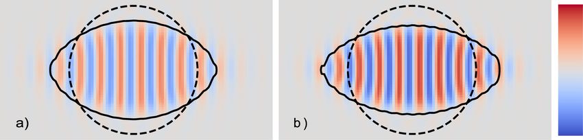
New J. Phys. 22 (2020) 052001

rather the control parameter drops from super- to subcritical values outside of a certain domain. Such
spatial restrictions have been so far mostly studied in quasi one-dimensional systems. There, smooth
control parameter drops may strongly narrow the wavenumber band of stable periodic patterns or may even
select a specific wave number out of it [26, 28, 29], while rapid drops can cause pinning effects [30]. There
are recent indications that in two-dimensional systems, control parameter drops can have orientational
effects on stripe patterns, similar to ‘real’ boundary conditions [31].
    Orientation effects for patterns at boundaries are closely related to the important fact that the
emergence of a stripe pattern in two spatial dimensions breaks the rotational symmetry of the respective
system. Here we ask the important question: if we consider domains with flexible boundaries, will the
spontaneous symmetry breaking effect of pattern formation lead to a preference of anisotropic shapes of
domains in which a stripe pattern forms? On general grounds, it is a completely unexplored question
whether, and if so how, finite amplitude patterns can act—via their universal properties—as a means to
shape the domains on which they ‘live’. There exist, however, experimental example systems. If—naturally
very deformable—liquid drops are placed on a surface and are shaken vertically, the so-called Faraday
instability causes oscillating, spatially periodic stripe patterns at the drop’s free surface [8]. Experiments [15,
16] and simulations [32] show that with increasing amplitude of the Faraday waves, the liquid drops of
originally circular cross-section (their three-dimensional shape being a spherical cap) deform to elliptical
and finally even worm-like shapes. Is this a general effect for patterns in deformable domains? If so, it would
be highly relevant for biology, where both single cells and whole organisms have to become both internally
structured and elongated (‘polarized’) by the intricately regulated interplay of, typically biochemical,
patterning and elastic deformations, the most important examples being cell division and symmetry
breaking in development [33]. Finally, understanding the generic properties of the ‘self-shaping’ of ‘active
domains’ may also give insights for the development of biomimetic approaches along the lines
of, e.g. [25].

2. Stripe patterns favour rectangular domains

Let us first recall the orientation of nonlinear stripe patterns with respect to boundary conditions in fixed
domains and demonstrate why stripes prefer rectangular, i.e. anisotropic domains. We choose the
Swift–Hohenberg (SH) model, known to capture the generic features of stationary stripe patterns
[5, 19, 34],

                                 ∂t u = β − (q20 + ∇2 )2 u − au3 − bu(∇u)2 .

                                                                                                               (1)

This equation for u(x, y, t) is isotropic in the x–y-plane and ±u symmetric. q0 is the preferred dimensionless
wave number of stripe solutions. These evolve for positive values of the control parameter, β > 0. Their
amplitude is limited by the cubic nonlinearities for a > 0, b > 0 (supercritical bifurcation).
    For b = 0 equation (1) is the common SH-model and follows a gradient dynamics, ∂t u = − δF     δu
                                                                                                     u
                                                                                                       , with
the functional
                                      1
                                        Z         h        a               2 i
                               Fu =        dx dy −βu2 + u4 − q20 + ∇2 u .                                     (2)
                                      2                    2

For b 6= 0 equation (1) is a generalization of the original SH model and includes non-potential effects [19].
The model was studied in reference [19] in rectangular domains R with u = ∂ n u = 0 along the boundaries
∂R, where ∂ n denotes the derivative normal to the boundaries. In this case, stripe patterns prefer to orient
perpendicularly to the boundary. Moreover, if the control parameter β in equation (1) varies from a
supercritical value inside a certain domain (β > 0) to a subcritical value outside (β < 0), e.g. as specified
below in equation (7), the stripes also preferably orient perpendicular to this ‘effective boundary’. This is in
agreement with results obtained for convection rolls in temperature-field ramps [35] and with studies of
turing patterns [31] near non-resonant control parameter ramps.
    The—completely generic—orientation of stripe patterns near boundaries can be understood as follows.
A supercritically bifurcating spatially periodic pattern (with equation (1) just being a representative) with
wave vector q0 = (q0 , 0) can be decomposed into a rapidly varying part exp(iq0 x) and a complex envelope
A(x, y, t), which is slowly varying on the length scale λ = 2π/q0 [2, 5, 36]. The envelope A follows the
Newell–Whitehead–Segel equation (NWSE) that covers the major properties of stripe patterns close to
threshold (including also the non-gradient case of equation (1) with b 6= 0). Importantly, the NWSE also
follows a gradient dynamics [2, 5]

                                              2
New J. Phys. 22 (2020) 052001
δF
τ0 ∂t A = − , with
δA∗
Z " 2#
1 2 g 4 i 2
FA = dx dy −ǫ|A| + |A| + ξ0 ∂x − ∂ A . (3)
2 2 2q0 y
We note that if the NWSE is derived from the dimensionless equation (1), one has τ 0 = 1, ε = β,
g = 3a + q20 b and ξ 0 = 2q0 .
Since its
pdynamics is relaxational, on sufficiently large domains R the NWSE has constant solutions
Ahom = ± ε/g in the bulk. What about the boundaries? According to the different orders of the
derivatives along the x and y-axis, the NWSE is anisotropic. By replacing x → x/lp and y → y/ln with
1/4
ξ02
ξ0
ln = √ , and lp = , (4)
ε 4q20 ε
and rescaling time and amplitude in the NWSE the coefficients in this equation have all the value ‘1’. Hence,
for a stripe pattern with wave vector q oriented normally (respectively parallely) to the domain boundary
∂R, its amplitude A decays to zero on a length scale ∝ ln (respectively ∝ lp ), see also appendix B. Since the
NWSE evolves towards the minimum of the functional FA , a stripe pattern prefers to stay at its bulk value
Ahom for a maximum possible area. Hence, due to the relation lp < ln for the decay along the boundaries,
the wave vector q preferentially aligns parallel to the interface and consequently the stripe pattern
perpendicular to it. p
Let us assume a fixed, rectangular area R = p Lx Ly with aspect ratio Γ = Lx /Ly and hence Ly = R/Γ. In
the bulk, the stripe pattern has amplitude A ∝ ε/g and FA ∝ ε2 R. In the case of the boundary condition
A = 0 along ∂R, or a control parameter ramp [31], the pattern decays across ∂R on the length scale ln or lp ,
depending on the orientation. With these lengths, and the approximation that at the interfaces the
functional is on average halved, the functional for the domain is proportional to
FA ∝ −ε2 R − ln Ly − lp Lx
(5)
1/4
with a minimum at a finite aspect ratio Γmin = 4q20 ξ02 /ε . The minimum as a function of Γ occurs, since
large aspect ratios are again unfavorable for the following reason: for narrow rectangles with a width
becoming of the order of a few lp , the stripes amplitude is suppressed, i.e. cannot reach the bulk value
anymore.
Therefore, a stripe pattern near threshold has a lower value of the functional FA on rectangular domains
Ly > Lx than on a square domain, at fixed area of the domain. This scaling result for supercritically
bifurcating stripe patterns in finite domains is universal and holds besides many systems described by the
NWSE [5] also for equation (1) and b 6= 0. We confirmed this result by simulating equation (1) in the case
of gradient dynamics (b = 0) and a control parameter defined as
β(x, y) = ε(2ρ(x, y) − 1) (6)
with
" ! !#
1 x + L2x x − L2x
ρ(x, y) = tanh p − tanh p
4 ξβ ξβ
" L
! L
!#
y + 2y y − 2y
× tanh p − tanh p (7)
ξβ ξβ
to implement a supercritical control parameter in the range [−Lx /2, Lx /2] × [−Ly /2, Ly /2] with the
domain area R = Lx Ly .
Keeping the size R of the domain fixed we determined the stationary solutions of equation (1) for
different values of Γ = Lx /Ly and the respective values of the functional Fu . The result for the functional is
shown in figure 1 as a function of Γ for different values of ε. These numerical results confirm the scaling
estimate from above, i.e. that for stripe patterns the functional in equation (2) has a minimum for finite
aspect ratios Γ > 1 of the domain. This line of arguments strongly suggests that stripe patterns will favor
anisotropic domains if the boundaries of their domain are movable or deformable by the pattern. We will
investigate this feedback of a pattern on its domain in the following sections in more detail.
3New J. Phys. 22 (2020) 052001
Figure 1. The (scaled) functional Fu in equation (2) as a function of the aspect ratio Γ = Lx /Ly at fixed area R = Lx Ly . Fu has
been evaluated for stationary stripe solutions of equation (1) for b = 0, using the control parameter ramps as given by
equation (7) and for three values of ε: ε = 0.1 (solid blue line), 0.2 (dashed orange line) and 0.4 (dashed-dotted green line).
Crosses mark the minimum of Fu . Other parameters: ξ β = 8, a = 1, q0 = 1 and b = 0.
3. Coupling of stripe patterns to deformable domain boundaries
A deformable finite domain R with a positive control parameter inside and a negative one outside can be
elegantly implemented by the so-called phase field method. This approach, originally developed for
solidification processes [37] has been applied in recent years to many soft matter [38] and biological
problems [39], for instance droplets and vesicles in flows [40] or cell motility [41]. It is a well-adapted
approach to self-consistently describe deformable and/or moving boundaries.
The idea is to render the function ρ(x, y), that occurs via equation (6) in the control parameter,
dynamic. The phase field ρ(x, y, t) has values ρ = 1 inside the given domain R, ρ = 0 outside and a diffuse
interface in between, the ρ = 1/2-isoline being identified with the domain boundary ∂R. The phase field
dynamics is over damped,
Z
δFρ Dρ 2
∂t ρ = − , with Fρ = f (ρ) + (∇ρ) dx dy. (8)
δρ 2
Rρ
Herein f (ρ) = 0 (1 − ρ′ )(δ − ρ′ )ρ′ dρ′ is the homogeneous energy density, having a double well structure
with minima at the ‘phases’ ρ = 1, 0. The gradient term in Fρ corresponds p to a wall energy penalizing
domain walls. Dp ρ determines the interface width (which in 1D is given by 2 2Dρ ) and the effective surface
tension (also ∝ Dρ ). More complex interfacial properties and feedbacks can be implemented [42], but we
here consider R only the simplest wall energy. The parameter δ occurring in the energy density is chosen as
δ = 12 − µ ρ dx dy − R0 . δ = 1/2 is the stationary point, where ρ = 0, 1 have equal energy and hence
flat interfaces are stationary. In fact, in 1D this choice leads to hyperbolic tangent solutions as assumed in
equation (7). The second term is a simple implementation of area conservation to a fixed value R0 with the
stiffness of the constraint given by µ (we here use µ = 0.1 throughout). We refer to appendix A for an
alternative implementation of an intrinsically conserved phase field, yielding qualitatively the same results
as equation (8).
Stripe patterns have a certain stiffness that tries to keep stripes straight and, as described above, they
prefer to orient themselves perpendicular to a domain boarder suppressing the patterns amplitude.
Accordingly, the intrinsic elasticity of stripe-pattern may cause deformations of a flexible domain boundary,
as they are described by the phase field. The preferred perpendicular orientation between domain
boundaries and stripe patterns has similarities with the homeotropic (perpendicular) orientation of
nematic liquid crystals at container boundaries for which there is a generic mean field description of the
coupling between the orientation of nematic liquid crystals and the container boundaries [43]. Translating
to our case, the orientation of the stripe pattern can be described by the direction of the patterns wave
vector, which is parallel to ∇u(r, t), and the orientation of the deformable domain boundary by its normal
∇ρ. Accordingly we add to the phase-field potential such a generic orientational contribution
α
Z
Fρcoupled = Fρ + (∇ρ · ∇u)2 dx dy, (9)
2
which leads to a feedback of the pattern on the domain shape and favours (vanishes for) the stripe’s wave
vector perpendicular to the boundary normal. Any other relative orientation costs energy with the stripe
orientation parallel to the domain boundary the most costly. The parameter α describes the coupling
strength. We note that the phase field acts back on the pattern field u only via the spatial variation of the
control parameter given by equation (6).
4New J. Phys. 22 (2020) 052001
Figure 2. Shown are two stationary solutions of equations (10) that have been obtained starting with a circular initial domain R
(marked dashed) and for a supercritical control parameter ε = 0.2. The coupling strength α = 6 in (a) leads to a final domain
shape with aspect ratio Γ = 1.4; the value α = 100 in (b) to Γ = 2.8. Other parameters: Dρ = 1, R0 = πr02 with r0 = 43; q0 = 1,
a = 1, b = 0.
The final generic model equations for a stripe pattern forming inside a deformable domain then read
∂t ρ = Dρ ∇2 ρ − (1 − ρ)(δ − ρ)ρ + α∇ · ([∇ρ · ∇u]∇u) ,
∂t u = ε(2ρ − 1) − (q20 + ∇2 )2 u − au3 − bu(∇u)2 ,
(10)
supplemented by the volume constraint δ as given above.
4. Stripe patterns within deformable domains
Starting simulations of the coupled model equation (10) with circularly shaped domains and with small
√
initial amplitudes for the stripes, we observe a rapid saturation of the stripe amplitude ∝ ε in the bulk of
the domain. After this initial phase of fast dynamics, the finite amplitude stripe pattern starts to deform the
flexible domain on a much slower time scale, according to the coupling parameterized by α. An initially
circularly shaped domain gets increasingly elongated to an elliptical shape by increasing the coupling
parameter α, as indicated in figure 2. In fact, due to this deformation of the domain, stripes can meet the
domain boundaries perpendicularly in a larger region. The elongation to elliptical shapes saturates at an
aspect ratio Γ > 1, as we already anticipated from the minimum of Fu at Γ > 1 for fixed rectangular
domains in figure 1. As indicated in figure 2, the final value of Γ increases with coupling strength α from
Γ = 1.4 at α = 6 in part (a) to Γ = 2.8 for α = 100 in part (b). It should also be noted that the deformed
domains allow the pattern forming system to fit in additional stripe units, i.e. wavelengths: for the example
shown in figure 2(b) from 14 within the circular domain to 24 stripe units.
As indicated in the introduction and in reference [31], rapid and smooth control parameter variations
have different effects on patterns and its orientations. In the generic model presented here, the control
parameter is directly slaved to the phase field interface. We now study both cases in more depth. We start
with the smooth interface case, for which Dρ = 1 as chosen for figure 2 is a good representative.
4.1. Smooth diffuse interfaces
How do pattern forming systems with deformable domains reach their stationary state in this case? We
started simulations (with b = 0) for different initial aspect ratios, namely with Γ = 1 below and with Γ = 3
beyond the final stationary value of Γ. We determined Fu (t) and Γ(t) as a function of time and show
Fu versus Γ in figure 3(a) for three different values of the control parameter ε and for α = 6. The bullets
(•) in each part of the figure mark the final stationary state. Note that this state does not correspond to the
minimum of Fu (Γ) (marked by ×), since Fu is not a potential for the full coupled dynamics, only for the
pattern formation part. In other words, Fu (Γ) does not reach its minimum, because the system reaches a
stationary state as soon as the surface tension-like forces induced by the deformation of the domain and
inherent to the phase field description balance the elongational forces induced by the energy gain of
orienting the stripes perpendicularly to the domain boundary.
Since the driving force for the deformation of the domain increases with increasing stripe amplitude
√
∝ ε, also the aspect ratio Γ at the stationary state (marked by •) increases with ε. On the other hand the
minimum of Fu (marked by ×) decreases with increasing ε and the mismatch between both decreases. Note
that, for particular parameters, here for ε = 0.4, the stationary state and the minimum can coincide as
indicated in figure 3(a). We find an analogous behavior in figure 3(b), where the control parameter was
5New J. Phys. 22 (2020) 052001
Figure 3. Shown is the rescaled functional F̃ u = Fu 100/ε2 per unit area for a stripe pattern as a function of the aspect ratio Γ of
the domain. The simulation was either started with a circular domain of aspect ratio Γ = 1 or an elliptical domain with Γ = 3.
In (a) F̃ and Γ where calculated as a function time for α = 6 and for different values of ε: ε = 0.1 (solid blue line), ε = 0.2
(dashed orange line), ε = 0.4 (dashed-dotted green line). The bullets (•) mark the final stationary solution, the crosses (×) the
minimum of F̃ u . Note that the bullet for the dashed line corresponds to the final solution shown in figure 2(b). Part (b) shows a
similar plot for a fixed control parameter ε = 0.1 and three values of the coupling strength: α = 6 (solid blue line), α = 30
(dotted red line) and α = 100 (dashed purple line). Further parameters: Dρ = 1, a = 1, b = 0, A = r02 π, r0 = 43.
Figure 4. Part (a) shows the aspect ratio Γ as a function of the coupling strength α for three different values of the control
parameter: ε = 0.1 (solid blue line), ε = 0.2 (dashed orange line) ε = 0.4 (dashed dotted green line) (a = 1, b = 0). Part (b)
shows Γ as a function of the control parameter for coupling strength α = 60 and three combinations of the nonlinear
coefficients: a = 1, b = 0 (solid blue line; corresponding to gradient dynamics), a = 1, b = 1 (dashed orange line), a = 13 , b = 1
(dashed dotted green line). Further parameters are: Dρ = 1, A = r02 π, r0 = 43.
fixed and the coupling strength α was varied: again a stronger effect of the pattern on the boundary by
increasing the coupling strength reduces the difference between the steady state value of Γ (at •) and the
corresponding minimum of Fu (Γ) (marked by ×).
In figure 4 we further quantify how a stripe pattern deforms its domain as function of the parameters.
Figure 4(a) shows the final aspect ratio Γ as a function of the coupling strength α for different values of the
control parameter ε and at fixed domain area R. The slope of the curves Γ(α) increases with ε, but the three
curves tend to saturate as a function of α at an upper limit of about Γmax ∼ 3. This saturation depends
essentially on the ratio between the short axis of the ellipse and the decay length lp . Accordingly, the
maximum stationary value of the aspect ratio Γmax will increase with the area R of the domain.
Figure 4(b) shows the final aspect ratio as a function of the control parameter ε for a fixed coupling
strength α = 60. Here, the solid curve corresponds to the case b = 0, exclusively studied so far,
corresponding to the case where equation (1) follows a gradient dynamics governed by equation (2). Both
the dashed and the dash-dotted curves have been obtained for the non-potential case (b 6= 0).
According to figure 4 the effect of the pattern on the boundary, as reflected by the aspect ratio Γ,
increases with both the coupling strength α and the pattern amplitude (respectively ε), before it reaches a
saturation level. Moreover, these parameter trends are quite similar for the case of gradient and
non-gradient dynamics. The pattern deforming its boundary to reduce the functional Fu is equivalent to its
6New J. Phys. 22 (2020) 052001
Figure 5. Shown is the time evolution of the wave number qs (t) of stripe patterns and the aspect ratio Γ(t) of the domain in the
plane qs vs Γ. Simulations of equation (10) with a = 1, b = 0 were started either with a circularly shaped domain, Γ = 1 (solid
lines), or with a strongly elliptically shaped domain, Γ = 4 (dashed lines). In both cases, stripe patterns of three different initial
wave numbers qinit = 0.96 (blue), qinit = 1.0 (orange) and qinit = 1.04 (green) were studied. In part (a) a smooth, diffuse
interface was implemented via Dρ = 1. In (b) Dρ = 0.4 was used, implying a steeper decay of the control parameter.
attempt to reach maximum amplitude in an as large as possible subdomain of R. This trend still holds in
the case of a non-gradient dynamics, where it again is achieved best with the stripe pattern staying
perpendicularly to the domain boundary.
4.2. Dynamical selection of aspect ratio and wave number
Both the aspect ratio Γ of the domain and the wave number q of the periodic pattern are dynamically
selected, as shown in figure 5(a) for the case of a smooth, diffuse control parameter variation across the
boundary, using Dρ = 1. In order to demonstrate this statement, we started two sets of simulations of
equation (10): on the one hand, we started with a circularly shaped initial domain and a finite amplitude
pattern with three different initial wave numbers (solid curves in figure 5(a)). In this case, Γ increases with
time until the differently started simulations meet at the same wave number: in fact, the system selects a
specific aspect ratio and a specific wave number. On the other hand, we started with periodic patterns of
three different wave numbers but now on a domain with a large aspect ratio Γ ∼ 4. Now, Γ decayed with
time and again the aspect ratio and the wave numbers evolved to the same value as before. One can hence
conclude that the selection process is robust with respect to the initial conditions.
From systems with fixed domain shapes in quasi one-dimension (1D) having smooth spatial parameter
variations, the phenomenon of a strong wave-number restriction or selection is well known [26–28].
However, that this behavior also generalizes for deformable two-dimensional systems to a simultaneous
selection of the aspect ratio and the wave number, independent of the initial conditions, is rather surprising.
In addition, there are two further aspects of wave number selection that are different to previous quasi
one-dimensional studies: first, in the quasi 1D case with gradient dynamics the preferred wave number, here
q0 = 1, is selected. This corresponds to the wave number where the pattern amplitude takes its
maximum as a function of q and the respective functional its minimum (also called the Eckhaus band
middle). In contrast, in the 2D deformable domain situation, even in the case of gradient dynamics, the
selected wave number q = 1.005 > q0 = 1 does not correspond to the wave number of maximum
amplitude or minimum functional.
Second, we note that in the non-gradient case with b 6= 0, the amplitude A of a periodic stripe pattern in
an extended system (cf u = Aeiqx + c c) is given by
ε − (q20 − q2 )2
A2 = . (11)
3a + bq2
For a > 0, b > 0, |A(q)| hence should take its maximum at a q < q0 = 1. Nevertheless, in our simulations of
equations (10) for b 6= 0, we again obtained (not shown) a selected wave number qs that is larger than q0
and even larger than the selected wave number in the case of gradient dynamics.
For more rapid and steep control parameter variations across the domain boundary (modeled by
smaller values of Dρ ), one still obtains a rather strict wave number selection, as shown in figure 5(b) for
Dρ < 0.4. However, the selected stationary aspect ratio depends now on the initial shape, as indicated by the
gap in figure 5(b), and on the steepness of the control parameter variation via Dρ . For smaller values of Dρ
the gap increases. In fact, from quasi-1D systems it is known that more rapid and steep parameter
variations may lead via pinning effects to an imperfect wave number selection [30]. We investigate the
dynamics in this regime in the next section.
7New J. Phys. 22 (2020) 052001
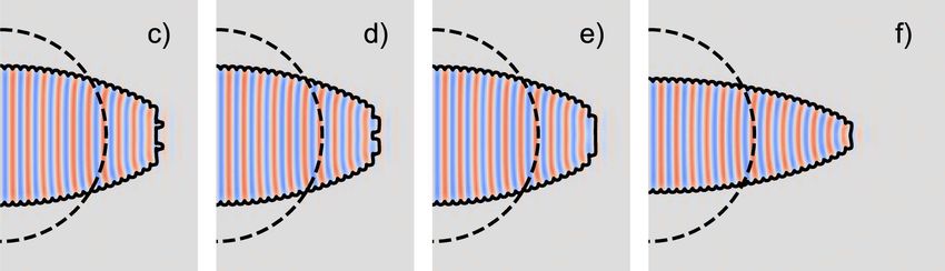
Figure 6. Simulation results for a steep phase field interface (Dρ = 0.1), resulting in a rapid decay of the control parameter
across the domain boundary. Panel (a) shows that periodic patterns are pinned for small values of the control parameter ε and
the initially circular domain remains essentially undeformed, i.e. the aspect ratio Γ stays close to one. Beyond a critical value of ε,
the pattern becomes depinned and Γ increases as indicated by (•) for a = 1, b = 0, i.e. gradient dynamics, by (×) for
a = 1/3, b = 1 and by (+) for a = 1, b = 1. The coupling strength was chosen to be α = 60. Panel (b) shows Γ(t) for ε = 0.2,
α = 60 and a = 1/3, b = 1. The slight modulations in the curve are a signature of weak pinning effects at the boundary. The
snapshots in (c)–(e) illustrate the complex evolution of the pattern during the propagation of the domain boundary at
intermediate times, cf crosses in the inset of part (b). Panel (f) displays the stationary final state for the same simulation.
4.3. Steep interfaces and pinning effects
During the evolution from the initially circularly shaped domain to an elliptical domain as exemplified in
figure 2(b), new periodic units appear rather smoothly due to the smooth diffuse control parameter
variations across the domain boundaries for Dρ = 1.0. When, in contrast, a rather steep phase field
variation across the boundary is chosen, as exemplified here by Dρ = 0.1, the periodic pattern may get
pinned at the resulting steep control parameter variations. Moreover, the pinning of the stripe pattern may
persist over a wide range of control parameters ε, as shown in figure 6(a): for small ε, no further periodic
units (wave lengths) can emerge and the aspect ratio Γ stays fixed close to its initial Γ ≃ 1. Beyond this
pinning regime, the pattern rapidly evolves to much larger values of Γ, as shown in figure 6(a) for three
different combinations of the nonlinear parameters a, b in equation (10), corresponding to both gradient
and non-gradient dynamics.
During this evolution, Γ increases with time as shown exemplarily in figure 6(b). Since the additional
periodic units emerge step by step, also the aspect ratio increases in a stepwise fashion, as highlighted by the
inset of the same panel. The respective snapshots given in figures 6(c)–(f) illustrate the complex
two-dimensional dynamics during the emergence of further periodic units—corresponding to the time
t = 1500–1700 shown in the inset of figure 6(b)—and, lastly, the finally obtained stationary state.
Note that, while we still found a unique wave-number selection for Dρ = 0.4 in figure 5, this unique
selection mechanism does in general not hold anymore for Dρ = 0.1 or smaller.
5. Discussion and conclusion
With the onset of nonlinear stripe patterns in two-dimensional domains, the rotational symmetry is broken.
In the often occurring case where the pattern forming field has to vanish outside the domain, this results in
an orientational preference for the stripes with respect to domain boundaries. We have shown here that this
fundamental property implies that stripe pattern prefer to ‘live in’ anisotropic domains. This insight then
motivated us to study deformable domains. We here applied a generic approach by coupling the
Swift–Hohenberg (SH) model to a phase field, describing the deformable domain, and implementing the
generic orientational preference of the stripes with respect to the domain boundaries by an energy inspired
from surface anchoring of liquid crystals. For both the gradient and a generalized non-gradient version of
the SH model we found that increasing either the pattern amplitude or the coupling strength deforms the
domain towards elliptical shapes of increasing aspect ratio. The deformation of the domain finally saturates
due to two effects: one is related to the fact that with increasing aspect ratio, the short elliptical axis reaches
8New J. Phys. 22 (2020) 052001
the range of the coherence length of the pattern along the stripe axis. In this regime the supercritical pattern
is prevented to reach its bulk amplitude, which is disfavored. The other effect is the surface or wall energy,
inherent to the phase field approach, which resists strong deformations. It should be noted that the latter
effect may not be present in some systems, but can also be removed from the phase field dynamics, cf
[42, 44].
From the generic modeling point of view, the phase field approach used here has another advantage: the
width of its diffuse interface can be tuned via the parameter Dρ . This allows us to make a connection to
previous works on the effects of control parameter ramps in pattern forming systems [26–28]. It is well
known that spatially periodic patterns in extended systems are stable for many different wave numbers out
of a stable, so-called Eckhaus band [5, 45–47]. In our present study we found the surprising result that the
wave number of the pattern and the domain shape described by the aspect ratio are selected simultaneously.
Furthermore, the selected wave number is larger than the one at the maximum of the amplitude (at the
minimum of the potential, in case it exists), irrespective whether the pattern follows gradient dynamics or
not. This is different from quasi one-dimensional pattern forming systems, where the wave number at the
minimum of the related potential is selected in case of gradient dynamics. Finally, in the case of steep
control parameter variations, slightly different domain shapes may be selected depending on initial
conditions, and an interesting step-wise dynamics of the domain deformation was observed.
The study of the generic effects of nonlinear stripe patterns in deformable domains undertaken here
shares many similarities with the specific example of Faraday waves emerging on top of shaken liquid
droplets [15, 16, 32]. However, Faraday waves on droplet surfaces are a three-dimensional situation. As long
as the contact area occupied by the drop does not change considerably, our findings should directly apply.
For larger drop deformations, the contact area increases and experimentally one finds worm-like droplets
and even drop splitting. Such situations could be taken into account within our generic model by
considering either three dimensional domains or a slow temporal dynamics for the area.
In conclusion, we studied a generic coupling of stripe patterns to the boundary of the deformable
domain wherein they form. Similarly interesting effects may also apply for traveling wave patterns [25, 48].
In addition, in the case of an externally forced boundary motion interesting reorientation effects may occur
at a sufficiently high boundary speed [49]. The fact that patterns are generically and inherently coupled to
the boundaries/surfaces of the ‘domains they live in’ should be further investigated, especially in view of
biological systems like the growing cells described in references [50, 51] or for the coupling of patterns on
interfaces and the domain shape, see e.g. reference [17].
Appendix A. Conserved phase field equation
In the main manuscript, we used an Allen–Cahn approach for the phase field, cf equation (8). The field
ρ(x, y) was hence not conserved a priori, but area conservation was implemented via the nonlocal term in
the definition of the parameter δ.
Another approach is the so-called Cahn–Hilliard model. Here the dynamics of the phase field is
explicitly conserved by writing
δFρ
∂t ρ = −∇2 . (A.1)
δρ
Due to the additional spatial derivatives, the model is numerically more involved, but we nevertheless
checked here whether the details of the phase field implementation matter for the overall dynamics of
patterns in deformable domains.
coupled
Using the same potential Fρ as before, but with constant δ = 21 , one arrives at the model equations:
2 2 1
∂t ρ = −∇ Dρ ∇ ρ − (1 − ρ) − ρ ρ + α∇ · ([∇ρ · ∇u]∇u) ,
2
∂t u = ε(2ρ − 1) − (q20 + ∇2 )2 u − au3 − bu(∇u)2 .
(A.2)
For finite values of the coupling strength α and positive control parameter ε, this model again prefers an
orientation of the stripe pattern perpendicular to the control parameter drop across the interface and
elongates the domain as shown in figure A1. The aspect ratio Γ of the stationary elongation increases with
both the coupling strength and the control parameter, as shown in figure A2.
Qualitatively, the behavior is identical to the one obtained using the model equation (10). The ‘global’
domain conservation in model equation (A.2) seems to lead to a stricter compliance with the form of the
interface. However, compared to model equation (10), the higher order derivatives in equation (A.2)
restricted our study to smaller control parameter values and system sizes.
9New J. Phys. 22 (2020) 052001
Figure A1. Shown are two stationary solutions of equation (A.2), both with the circular initial domain marked as dashed. The
control parameter was chosen to be ε = 0.2 and the coupling strength α = 6 in (a) vs α = 100 in (b), leading to increasingly
deformed domains (solid curves mark the ρ = 1/2-isocurves). Other parameters: Dρ = 1, R0 = πr02 with r0 = 20, q0 = 1, a = 1,
b = 0.
Figure A2. Panel (a) shows the aspect ratio Γ of stationary solutions of equation (A.2) for a = 1, b = 0 as a function of the
coupling strength α for ε = 0.05 (blue), ε = 0.1 (orange) and ε = 0.15 (green). In (b) Γ is given for a fixed coupling strength
α = 10 as a function of the control parameter ε for a = 1, b = 0 (blue), a = 1, b = 1 (orange) and a = 31 , b = 1 (green). Other
parameters as in figure A1.
Figure B1. Shown is a stripe pattern as obtained from simulations of equation (10) with q perpendicular to the boundary in
part (a) and parallel in part (b). The vertical lines mark the domain boundary at ρ = 0.5. The red dotted line in (a) describes the
x-dependence of the envelope A(X) and the blue line in (b) the envelope A(Y). Parameters: a = 1, b = 0, ε = 0.1, Dρ = 1.
Appendix B. Decay lengths of the amplitude
The explicit form of the NWSE (3) is given by
2
i 2
τ0 ∂t A = εA − ξ02 ∂x − ∂ A − g|A|2 A. (B.1)
2q0 y
By rescaling the spatial coordinate x resp. y by the lengths ln resp. lp given by equation (B.1) as well as time
and amplitude, the coefficients in equation (B.1) become all ‘1’. For the parameters q0 = 1 and ε = 0.1 the
length scale lp ≃ 1.78 for stripes perpendicular to the boundary (i.e. q parallel to the boundary) is smaller
10New J. Phys. 22 (2020) 052001
than parallel to it with ln ≃ 6.32. This results in different decay lengths of a stripe pattern parallel or
perpendicular to a boundary with a control parameter drop as illustrated by a simulation of equation (10)
for the parameter set in figure B1.
ORCID iDs
Falko Ziebert https://orcid.org/0000-0001-6332-7287
Walter Zimmermann https://orcid.org/0000-0001-7826-4629
References
[1] Ball P 1998 The Self-Made Tapestry: Pattern Formation in Nature (Oxford: Oxford University Press)
[2] Cross M C and Greenside H 2009 Pattern Formation and Dynamics in Nonequilibrium Systems (Cambridge: Cambridge University
Press)
[3] Meron E 2015 Nonlinear Physics of Ecosystems (Boca Raton, FL: CRC Press)
Meron E 2019 Phys. Today 72 30
[4] Lappa M 2009 Thermal Convection: Patterns, Evolution and Stability (New York: Wiley)
[5] Cross M C and Hohenberg P C 1993 Rev. Mod. Phys. 65 851
[6] Bodenschatz E, Zimmermann W and Kramer L 1988 J. Phys. 49 1875
[7] Kramer L and Pesch W 1995 Annu. Rev. Fluid Mech. 27 515
[8] Kudrolli A and Gollub J P 1996 Physica D 97 133
[9] St Johnston D and Nüsslein-Volhard C 1992 Cell 68 201
[10] Kondo S and Miura T 2010 Science 329 1616
[11] Loose M, Fischer-Friedrich E, Ries J, Kruse K and Schwille P 2008 Science 320 789
[12] Edelstein-Keshet L, Holmes W R, Zajak M and Dutot M 2013 Philos. Trans. R. Soc., B 368 20130003
[13] Bergmann F, Rapp L and Zimmermann W 2018 Phys. Rev. E 98 072001(R)
[14] Bergmann F and Zimmermann W 2019 PLOS ONE 14 e0218328
[15] Pucci G, Fort E, Amar M B and Couder Y 2011 Phys. Rev. Lett. 106 024503
[16] Hemmerle A, Froehlicher G, Bergeron V, Charitat T and Farago J 2015 Europhys. Lett. 111 24003
[17] Mietke A, Jülicher F and Sbalzarini I F 2019 Proc. Natl Acad. Sci. USA 116 29
[18] Kramer L and Hohenberg P C 1984 Physica D 13 352
[19] Greenside H and Coughran W M 1984 Phys. Rev. A 30 398
[20] Cross M C, Daniels P G, Hohenberg P C and Siggia E D 1983 J. Fluid Mech. 55 155
[21] Cross M C 1982 Phys. Fluids 25 936
[22] Bajaj K M, Mukolobwiez N, Currier N and Ahlers G 1999 Phys. Rev. Lett. 83 5282
[23] Chiam K H, Paul M R, Cross M C and Greenside H 2003 Phys. Rev. E 67 056206
[24] Munuzuri A P, Dolnik M, Zhabotinsky A M and Epstein I R 1999 J. Am. Chem. Soc. 121 8065
[25] Schweizer J, Loose M, Bonny M, Kruse K, Mönch I and Schwille P 2012 Proc. Natl Acad. Sci. USA 109 15283
[26] Kramer L, Ben-Jacob E, Brand H and Cross M C 1982 Phys. Rev. Lett. 49 1891
[27] Cannell D S, Dominguez-Lerma M A and Ahlers G 1983 Phys. Rev. Lett. 50 1365
[28] Riecke H and Paap H G 1987 Phys. Rev. Lett. 59 2570
[29] Cross M C 1984 Phys. Rev. A 29 391
[30] Riecke H and Paap H G 1986 Phys. Rev. A 33 547
[31] Rapp L, Bergmann F and Zimmermann W 2016 Europhys. Lett. 113 28006
[32] Pototsky A and Bestehorn M 2018 Europhys. Lett. 121 46001
[33] Gross P, Kumar K V and Grill S W 2017 Annu. Rev. Biophys. 46 337
[34] Swift J B and Hohenberg P C 1977 Phys. Rev. A 15 319
[35] Bodenschatz E, Pesch W and Ahlers G 2000 Annu. Rev. Fluid Mech. 32 709
[36] Newell A C and Whitehead J A 1969 J. Fluid Mech. 38 279
[37] Karma A and Rappel W J 1998 Phys. Rev. E 57 4323
[38] Emmerich H 2008 Adv. Phys. 57 1
[39] Ziebert F and Aranson I S 2016 npj Comput. Mater. 2 16019
[40] Biben T and Misbah C 2003 Phys. Rev. E 67 031908
[41] Ziebert F, Swaminathan S and Aranson I S 2012 J. R. Soc. Interface 9 1084
[42] Winkler B, Aranson I S and Ziebert F 2016 Physica D 318 26
[43] de Gennes P G and Prost J 1993 The Physics of Liquid Crystals (Oxford: Clarendon)
[44] Folch R, Casademunt J, Hernandez-Machado A and Ramirez-Piscina L 1999 Phys. Rev. E 60 1724
[45] Lowe M and Gollub J P 1985 Phys. Rev. A 31 3893
[46] Kramer L and Zimmermann W 1985 Physica D 16 221
[47] Dominguez-Lerma M A, Cannell D S and Ahlers G 1986 Phys. Rev. A 34 4956
[48] Bergmann F, Rapp L and Zimmermann W 2018 New J. Phys. 20 072001
[49] Avery M, Goh R, Goodloe O, Milewski A and Scheel A 2019 SIAM J. Appl. Dyn. Syst. 18 1078
[50] Raskin D M and de Boer P A J 1999 Proc. Natl Acad. Sci. USA 96 4971
[51] Murray S M and Sourjik V 2017 Nat. Phys. 13 1006
11You can also read