The non Newtonian maxwell nanofluid flow between two parallel rotating disks under the effects of magnetic field - Nature
←
→
Page content transcription
If your browser does not render page correctly, please read the page content below

www.nature.com/scientificreports

                OPEN              The non‑Newtonian maxwell
                                  nanofluid flow between two
                                  parallel rotating disks
                                  under the effects of magnetic field
                                  Ali Ahmadian1, Muhammad Bilal2, Muhammad Altaf Khan3,4* & Muhammad Imran Asjad5
                                  The main feature of the present numerical model is to explore the behavior of Maxwell nanoliquid
                                  moving within two horizontal rotating disks. The disks are stretchable and subjected to a magnetic
                                  field in axial direction. The time dependent characteristics of thermal conductivity have been
                                  considered to scrutinize the heat transfer phenomena. The thermophoresis and Brownian motion
                                  features of nanoliquid are studied with Buongiorno model. The lower and upper disk’s rotation for
                                  both the cases, same direction as well as opposite direction of rotation is investigated. The subsequent
                                  arrangement of the three dimensional Navier Stoke’s equations along with energy, mass and Maxwell
                                  equations are diminished to a dimensionless system of equations through the Von Karman’s similarity
                                  framework. The comparative numerical arrangement of modeled equations is further set up by built-in
                                  numerical scheme “boundary value solver” (Bvp4c) and Runge Kutta fourth order method (RK4). The
                                  various physical constraints, such as Prandtl number, thermal conductivity, magnetic field, thermal
                                  radiation, time relaxation, Brownian motion and thermophoresis parameters and their impact are
                                  presented and discussed briefly for velocity, temperature, concentration and magnetic strength
                                  profiles. In the present analysis, some vital characteristics such as Nusselt and Sherwood numbers are
                                  considered for physical and numerical investigation. The outcomes concluded that the disk stretching
                                  action opposing the flow behavior. With the increases of magnetic field parameter M the fluid velocity
                                  decreases, while improving its temperature. We show a good agreement of the present work by
                                  comparing with those published in literature.

                                  List of symbols
                                  ε	Thermal conductivity
                                  Λ	Pressure gradient parameter
                                  g	Transform azimuthal velocity
                                  q	Heat flux
                                  σ	Fluid electric conductivity
                                  η	Dimensionless variable
                                  Rd	Radiation parameter
                                  Ω1	Rotation rate of lower disk
                                  DB	Brownian diffusion coefficient
                                  K(T)	Variable thermal conductivity
                                  ρ	Fluid density
                                  λ1	Relaxation time parameter
                                  Nb	Brownian motion parameter
                                  DB	Brownian diffusion coefficient
                                  V	Kinematic viscosity
                                  T	Temperature

                                  1
                                   Institute of Industry Revolution 4.0, The National University of Malaysia, 43600 UKM Bangi, Selangor,
                                  Malaysia. 2Department of Mathematics, City University of Science and Information Technology, Peshawar,
                                  Pakistan. 3Informetrics Research Group, Ton Duc Thang University, Ho Chi Minh City, Vietnam. 4Faculty of
                                  Mathematics and Statistics, Ton Duc Thang University, Ho Chi Minh City, Vietnam. 5Department of Mathematics,
                                  University of Management and Technology, Lahore, Pakistan. *email: muhammad.altaf.khan@tdtu.edu.vn

Scientific Reports |   (2020) 10:17088              | https://doi.org/10.1038/s41598-020-74096-8                                            1

                                                                                                                                        Vol.:(0123456789)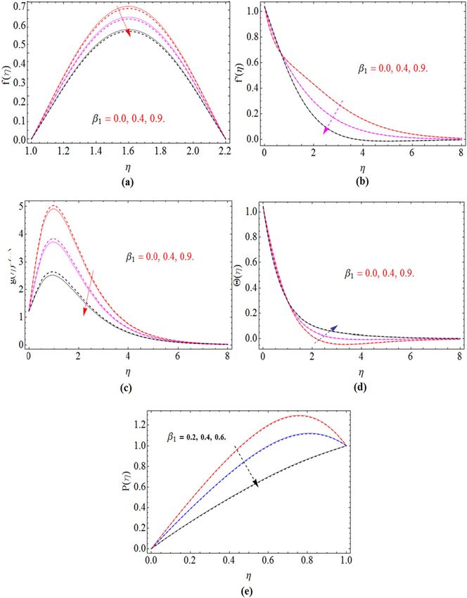
www.nature.com/scientificreports/
DT Coefficient of thermophoretic diffusion
Sc Schmidt number
T1 Temperature of Lower disk
Bt Batclor number
Φ,Θ Transform concentration & temperature
r, Θ, z Cylindrical coordinate system
Cp Specific heat
M Magnetic parameter
P Pressure
Ω Rotation parameter
d Vertical distance between disks
J Current density
B0 Strength of magnetic field
Ω2 Rotation rate of upper disk
Nabla Nabla
Pr Prandtl number
C Concentration
β1 Deborah number
Nt Thermophoresis parameter
DT Thermophoretic diffusion coefficient.
μ Dynamic viscosity
V Velocity vector
k Thermal conductivity
Re Reynolds number
T2 Temperature of upper disk
Rem Magnetic Reynolds number
f, f′ Transform axial and radial velocity
u, v, w Velocity components
The study of the fluid flow on the surface of rotating disk has got great attentions around the globe from the
researcher’s due to its many applications in practical problems. Electric power generating system, rotating
machinery, co rotating turbines, chemical process and computer storage, in the field of aerodynamics engineering,
geothermal industry, for lubrication purposes, over the surface of rotating disk the fluid flow is widely applicable.
Von Karman’s1 examined the solution of Navier stoke’s equations by considering an appropriate transformation.
Further, he used the fluid flow over the rotating frame for the first time. The Von Karman’s problem and its solu-
tion numerically have been discussed by Cochran2. Also, he used two series expansion by solving the limitation
in the Von Karman’s work. Sheikholeslami et al.3 used numerical technique for the solution of nanofluid flow
over an inclined rotating disk. During the rotation of the disk, Millsaps and Pahlhausen4 studied the heat trans-
port characteristic. The electric field in radial direction has been considered by T urkyilmazoglu5, where the heat
transfer phenomena in magnetohydro-dynamic (MHD) fluid flow has been investigated. Under the transverse
magnetic field influence, Khan et al.6 considered the non-Newtonian Powell-Eyring fluid over the rotating disk
surface. The entropy generation due to porosity of rotating disk in MHD flow has been investigated by Rashidi et
al7. Hayat et al.8 scrutinized the transfer of heat with viscous nanoliquid among two stretchable rotating sheets.
The thermal conductivity that depends on temperature in Maxwell fluid over a rotating disk has been studied by
Khan et al.9. Batchelor10 was the first researcher, who discussed the fluid flow between the gaps of the rotating
frame. The influence of blowing with wall transpiration, suction and mixed convection has investigated by Yan
and Soong11. Recently Shuaib et al12. studied the fractional behavior of fluid flow through a flexible rotating disk
with mass and heat characteristics.
The attention of researcher’s is increasing towards nanofluid studies day by day due to its many applications in
technology that binging facilities in many industrial process of heat transfer. The applications of nanofluid are in
drugs delivery, power generation, micromanufactoring process, metallurgical sectors, and thermal therapy, etc.
Choi13 is a researcher who worked for the first time on nanofluid, where he considered it for cooling and coolant
purpose in technologies. He found from his work that in a base fluid (water, oil and blood, etc.) by adding the
nanoparticles, the heat transfer of thermal conductivity becomes more effective. Using the idea of Choi’s idea,
many researchers investigated and obtained results using the n anofluids14,15. A concentric circular pipe with
slip flow has been discussed in T urkyilmazoglu . By using finite element method (FEM), Hatami et al.17 finds
16
the solution for the heat transfer in nanofluid with free natural convective in a circular cavity. The Cattaner-
Christov heat flux and thermal radiation for an unsteady squeezing MHD flow has been considered by Ganji
and Dogonchi18. They considered the heat of transfer of the nanofluid among two plates. Dilan et al.19 studied
nanofluids effective viscosity based on suspended nanoparticles. A carbon nanotubes based multifunctional
hybrid nanoliquid has been considered by Rossella20. The influence of SWCNTs on human epithelial tissues is
studied by Kaiser et al21. Hussanan et al.22 examined the Oxide nanoparticles for the enhancement of energy in
engine nanofluids, kerosene oil and water. Saeed et al.23 examined nanofluid to improve the heat transfer rate and
reduce time for food processing in the industry. Some recent studies related to heat and mass transfer through
nanofluids are examined by many r esearchers24–28.
To study the behavior, impact and properties of magnetic field over viscous fluids is known as MHD. Salt water,
plasmas and electrolytes are the examples of magnetofluids. . In the present era, the researchers and investigators
are taking very keen interest in this field. A lot of work has been done in this area. The tectonic applications of
Scientific Reports | (2020) 10:17088 | https://doi.org/10.1038/s41598-020-74096-8 2
Vol:.(1234567890)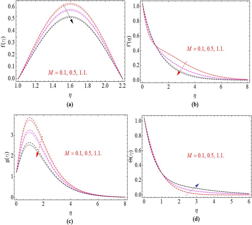
www.nature.com/scientificreports/
MHD in engineering, chemistry, physics, industrial tackle and in many other fields, for instance, pumps, bearings,
MHD generators and boundary layer control are contrived by the intercourse of conducting fluid and magnetic
field. In affiliation with these applications, the work of numerous explores has been deliberated. The most essential
and consequential challenge is the hydro magnetic behavior of boundary layers with the magnetic field transversely
along the moving surfaces or fixed surfaces.Hannes Alfén29 was the first one to innovate the MHD field. In 1970
he received the Nobel Prize in physics because of his innovation in MHD field. In Medical Sciences the applica-
tions of MHD fluid flow in distinguishable configuration pertinent to human body parts are very fascinating and
tectonic in the scientific area. The important applications of MHD in peristaltic flow, pulsatile flow, simple flow
and drug delivery are explored by Rashidi et al30. The numerical solution has been presented by Nadeem et al.31 for
the nanoparticles with different base fluids with slip and MHD effect. Khatsayuk et al.32 has explored the numeri-
cal simulation of MHD vortex technology and its verification is also ensured. The main of letters portrays casting
principle into the electromagnetic mold to invoke small diameter ingots33. Deng and W. M. Liu et al.34–37 have
presented the numerical and theoretical analysis in a rotating Bose–Einstein of the quantized vortices condensate
with modulated interaction in anharmonic and harmonic potentials. They further scrutinized the nonlinear matter
of the quasi-2D Bose–Einstein condensates with nonlinearity in the harmonic potential. They concluded that all
of the Bose–Einstein condensates have discrete energies with an arbitrary number of localized non-linear matter
waves, which are the exact solutions of the mathematical Gross-Pitaevskii equation.
Our inspiration of the present work is to analyze and model the Maxwell nano liquid flow within two stretch-
able coaxially rotating disks. The second priority is to initiate three dimensional Maxwell equation along with the
Navier stokes equation for such type of flow and set up an arrangement for temperature, concentration, velocity
and magnetic strength profile. For comparative results the built-in numerical scheme bvp4c and RK4 are opt-
ing. We have extended the idea of Ahmed ET al.38 and portrayed this mathematical model. The commitments
flow factors on velocity, temperature, concentration, pressure and magnetic strength profile are studied and via
graphical and in tabulated form. In the next section, the problem will be formulated and discussed.
Mathematical formulation of the problem. We assumed the nanoliquid steady motion within, the two
horizontal parallel rotating disks. The disks are stretchable and subjected to magnetic field B0 in axial direction.
The upper disk is considered at a constant position z = d, while the lower disk is at z = 0. The stretching rate and
velocity during rotation are (S1 , �1 ), while stretching rate and rotation velocity of upper disk are (S2 , �2 ). The
concentration and temperature of the lower and upper disk are respectively given by (C1 , C2 ) hand (T1 , T2 ). The
geometry of the considered problem is shown in Fig. 1. The governing equation of nanofluid flows a re9,39
∂u u ∂w
+ + = 0, (1)
∂r r ∂z
∂u ∂u u2 1 ∂P ∂ 2u ∂ 2u ∂ ∂w 2 ∂u 2u
u +w − =− + ν(2 2 + 2 + ( )+ − 2)
∂r ∂z r ρ ∂r ∂r ∂z ∂r ∂z r ∂r r
2
∂ u ∂ 2 u ∂ ∂u 2uv ∂v 2vw ∂v uv 2 v 2 ∂u
− 1 (u2 2 + w 2 2 + 2uw ( ) − − + 2 + ) (2)
∂r ∂z ∂r ∂z r ∂r r ∂z r r ∂r
σ2
− ρ(u + w 1 u2 ),
B0
∂v ∂v uv ∂ 2v v ∂ 2 u 1 ∂v ∂ 2v ∂ 2v
u +w − = ν(2 2 + 2 + 2 + ) − 1 (u2 2 + w 2 2
∂r ∂z r ∂r r ∂z r ∂r ∂r ∂z
(3)
∂ ∂v 2uv ∂v 2vw ∂u u2 v v 2 ∂v σ2
+2uw ( ) − − −2 2 + )− ρ(v + w 1 v2 ),
∂r ∂z r ∂r r ∂z r r ∂r B0
∂w ∂w 1 ∂P ∂ ∂u ∂ 2w 1 ∂u 1 ∂w ∂ 2w
u +w =− + ν( ( ) + 2 + + +2 2 )
∂r ∂z ρ ∂z ∂r ∂z ∂r r ∂z r ∂r ∂z
2 2 2
(4)
∂ w ∂ v ∂ ∂w v ∂w
− 1 (u2 2 + 2 + 2uw ( )+ ),
∂r ∂z ∂r ∂z r ∂r
∂T ∂T k(T) ∂T ∂ ∂T ∂ ∂T
(ρcp )f (u +w )= + (k(T) ) + (k(T) )
∂r ∂z r ∂r ∂r ∂r ∂r ∂z
∂T ∂C ∂T ∂C DT ∂T 2 ∂T 2 (5)
+(ρcp )p [DB ( + )+ {( ) + ( ) }],
∂z ∂z ∂r ∂r T2 ∂z ∂r
∂C ∂C ∂ 2C 1 ∂C ∂ 2C DB ∂ 2 T 1 ∂T ∂ 2T
u +w = DB ( 2 + + 2 )+ ( 2 + + 2 ), (6)
∂r ∂z ∂r r ∂r ∂z T2 ∂r r ∂r ∂z
∂Br ∂w ∂Bz ∂u 1 ∂ 2 Br ∂ 2 Br 1 ∂Br Br
−w − Br +u + Bz + ( 2 + 2
+ − 2 ) = 0, (7)
∂z ∂z ∂z ∂z σ µ2 ∂r ∂z r ∂r r
Scientific Reports | (2020) 10:17088 | https://doi.org/10.1038/s41598-020-74096-8 3
Vol.:(0123456789)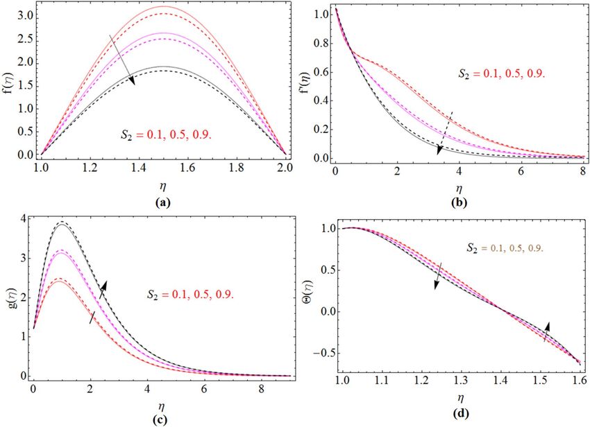
www.nature.com/scientificreports/
Figure 1. Geometry of the problem.
∂Bθ ∂u ∂Br ∂v ∂Bz ∂v ∂Bθ ∂w
−u − Bθ +v + Br +v + Bz −w − Bθ
∂r ∂r ∂r ∂r ∂z ∂z ∂z ∂z
(8)
1 ∂ 2 Bθ ∂ 2 Bθ 1 ∂Bθ Bθ
+ ( + + − 2 ) = 0,
σ µ 2 ∂r 2 ∂z 2 r ∂r r
∂Br ∂w 1 ∂Bz ∂u 1 1 ∂ 2 Bz ∂ 2 Bz 1 ∂Bz
w + Br + wBr − u + Bz − uBz + ( 2 + + ) = 0, (9)
∂r ∂r r ∂r ∂r r σ µ2 ∂r ∂z 2 r ∂r
where T represent the fluid temperature. The nanofluid heat capacity and base fluid specific heat are ρCp nf and
ρCp f respectively. The heat flux q is defined as
q = −∇Tk(T), (10)
In which variable thermal conductivity k(T) can be written as9
T − T2
k(T) = k∞ (1 + ε ). (11)
T1 − T2
ε Is the parameter of variable thermal conductivity and k∞ is the fluid thermal conductivity.
The boundary conditions are:
u = s1 r, v = ω1 r, w = 0, T = T1 , C = C1 , Br = 0, Bz = 0 at z = 0
dM0 (12)
u = s2 r, v = ω2 r, w = 0, T = T2 , C = C2 , Br = , Bz = −αM0 , at z = d.
2R
Scientific Reports | (2020) 10:17088 | https://doi.org/10.1038/s41598-020-74096-8 4
Vol:.(1234567890)
www.nature.com/scientificreports/
Transformation. The transformation, which are adopted to make the system of PDE dimensionless are as
follow38:
z
u = r� 1 f ′ (η), v = r� 1 g(η), w = −2d� 1 f (η), η =
d
1r 2 T − T1 C − C1
p = ρ� 1 v(P(η) + ), �(η) = , φ(η) = (13)
2 d2 T1 − T2 C1 − C2
�
′
Br = r�M0 M (η), Bθ = r�M0 N(η), Bz = M0 (2νf �)M(η).
The required dimensionless form of the system of differential equations given in Eqs. (1–9) are:
Re((f ′ )2 − g 2 − 2ff ′′ ) − Re(4ff ′ f ′′ − 4fgg ′ ) + MRe(f ′ − 2β1 ff ′′ ) − �
f ′′′ = (14)
1 − 4Reβ1 f 2
−2Re(fg ′ − f ′ g) − Reβ1 (4ff ′ g ′ + 4ff ′′ g) + MRe(g − 2β1 fg ′ )
g ′′ = (15)
1 − 4Reβ1 f 2
P ′ = −2f ′′ − Re(4ff ′ − 8β1 f 2 f ′′ ), (16)
−2Re Pr f �′ − ε�′2 − Pr Nb�′ �′ + Pr Nt�′2
�′′ = (17)
1 + ε�
Nt ′′
′′ = −2ReScf ′ −
, (18)
Nb
M ′′′′ = −2ReBt(Mf ′′′ + f ′′ M ′ − fM ′′′ − M ′′ f ′ ), (19)
N ′′ = 2ReBt(Mg ′ − fN ′ ), (20)
with condition
f (0) = 0, f ′ (0) = S1 , g(0) = 1, P(0) = 1, �(0) = 1, �(0) = 1, M ′ (0) = 0, N(0) = 0,
at η = 0
′ ′ (21)
f (1) = 0, f (1) = S2 , g(1) = �, �(1) = 0, �(1) = 0, M (1) = 1, N(1) = 1,
at η = d
The magnetic field M , Deborah number β1, lower and upper disks stretching parameters S1 and S2, param-
eter of Brownian motion Nb, Reynolds number Re, thermophoresis parameter Nt and Schmidth number Sc are
defined as:
σ B02 s1 s2 DB (C1 − C2 ) ρcp p
M= , β1 = 1 �1 , S1 = , S2 = , Nb =
,
ρ�1 �1 �2 ν ρcp f
(22)
DB (T1 − T2 ) ρcp p �1 d 2 ν
Nt =
, Re = , Sc = .
νT2 ρcp f ν DB
Sherwood and Nusselt numbers. The mass and rate of heat transfer for both disks can be illustrated a s38:
h ∂C h ∂T
Shr1 =− , Nur1 = − , atz = 0,
k(C1 − C2 ) ∂z k(T1 − T2 ) ∂z
(23)
h ∂C h ∂T
Shr2 =− , Nur2 = − , atz = d.
k(C1 − C2 ) ∂z k(T1 − T2 ) ∂z
The dimensionless form of Sherwood and Nusselt numbers can be written as
Shr1 = −�′ (0), Nur1 = −�′ (0),
(24)
Shr2 = −�′ (1), Nur2 = −�′ (1).
Scientific Reports | (2020) 10:17088 | https://doi.org/10.1038/s41598-020-74096-8 5
Vol.:(0123456789)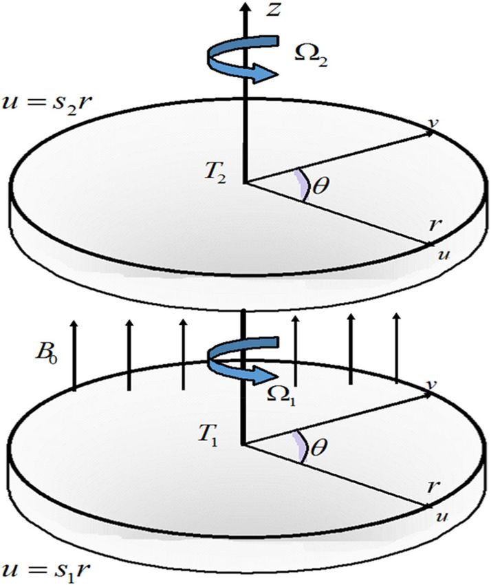
www.nature.com/scientificreports/

                                            Figure 2.  β1 impact on axial f (η), radial f ′ (η) and azimuthal velocity g(η), temperature �(η) and pressure
                                            profile P(η), for S2, when S1 = 0.0. dashed lines for  = 0.5 and lines for  =  − 0.5.

                                            Graphical interpretation
                                            Results and discussions. The governing equations of Non-Newtonian Maxwell nanofluid flow problem
                                            has been solved numerically using bvp4c scheme after using Karman’s scaling approach. In this section the
                                            results are illustrated through tables and Figures to visualize the impact of different physical constraints on
                                            velocity, pressure, concentration, temperature and magnetic strength profile. Both cases of disks rotation, same
                                            (� = 0.5) and in opposite direction (� = −0.5) of rotation has been sketched in Figs. 2, 3, 4, 5, 6, 7, 8. The entire
                                            calculation has been performed by keeping the values of constraints as Re = 4.0, M = 0.3, Nb = Nt = 0.3, β1 = 0.2,
                                            S1 = S2 = 0.4, ε = 0.1 and Sc = 3.0.

          Scientific Reports |   (2020) 10:17088 |               https://doi.org/10.1038/s41598-020-74096-8                                                    6

Vol:.(1234567890)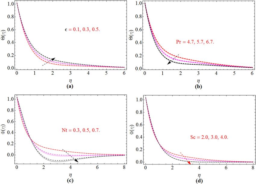
www.nature.com/scientificreports/

                                  Figure 3.  M impact on an axial f (η), radial f ′ (η) and azimuthal velocity g(η) and temperature profile �(η), for
                                  S2, when S1 = 0.0. dashed lines for  = 0.5 and lines for  =  − 0.5.

                                       Figure 2a–e are plotted, in order to illustrate the influence of Deborah number β1 on axial velocity profile
                                   f (η), radial f ′ (η) and azimuthal velocity g(η), temperature �(η) and pressure profile P(η) respectively. The
                                  fluid behaves as a solid substance with high Deborah number β1 shown in Fig. 2a. That’s why axial velocity
                                  reduces with the increases of β1. The fluid with low Deborah number possess less elastic property and vice versa
                                  illustrated in Fig. 2b,c. So the radial velocity and azimuthal velocity reduces with the improvement of β1. The
                                  fluid temperature is rises with β1 shown in Fig. 2d. The pressure profile of fluid decline with the rising values of
                                  Deborah number β1 Fig. 2e.
                                       Figure 3a–d demonstrate the behavior of axial velocity profile f (η), radial f ′ (η), azimuthal velocity g(η) and
                                  the temperature �(η) versus magnetic parameter M. The axial velocity and radial velocity decline with the effects
                                  of magnetic parameter M see Fig. 3a,b. Because the magnetic field creates some resistive forces, which oppose
                                  the fluid velocity and as a result axial and radial velocity reduces. The same trend has been received of azimuthal
                                  velocity via M Fig. 3c. By the enhancement of magnetic strength on the fluid flow generate friction, which pro-
                                  duces some amount of heat and as a result the average temperature of the fluid increases which is given in Fig. 3d.
                                       The dominance of Reynolds number against axial velocity, radial and azimuthal velocity is elaborated in
                                  Fig. 4a–c. Figure 4d elaborated to observe that the temperature field decline with the rising credit of Reynolds
                                  number (Re). The pressure profile of fluid also decline with the rising values of Reynolds number Fig. 4e.
                                       The two different cases for S2, when the lower disk stretching rate is (S1 = 0) and when it is (S1 = 0.5) have
                                  been sketched in Figs. 5a,b and 6a,b. In both cases the axial and radial velocity of fluid decreases with the improv-
                                  ing values of S2. While in azimuthal velocity an opposite seen has been observed, because by increasing stretching
                                  rate S2 the kinematics energy of fluid increases which enhanced the azimuthal velocity g(η) illustrated in Figs. 5c
                                  and 6c. Figures 5d and 6d are sketched to observe the upper disk stretching impact versus temperature profile,
                                  while keeping the lower disk stretching rate (S1 = 0) and (S1 = 0.5) respectively. When the disk stretch the fluid
                                  particle above the disk surface get some space and become relaxed for a while, as a result their temperature
                                  reduce, which causes the average temperature of fluid to reduce.

Scientific Reports |   (2020) 10:17088 |               https://doi.org/10.1038/s41598-020-74096-8                                                     7

                                                                                                                                                 Vol.:(0123456789)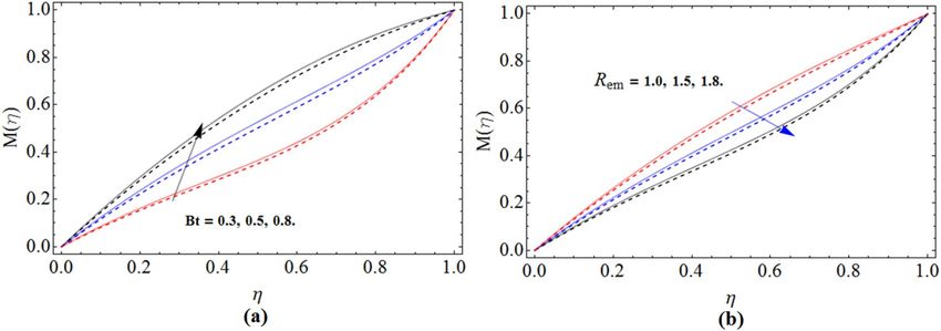
www.nature.com/scientificreports/

                                            Figure 4.  Re impact on axial f (η), radial f ′ (η) and azimuthal velocity g(η), temperature profile �(η) and
                                            pressure profile P(η), for S2, when S1 = 0.0. dashed lines for  = 0.5 and lines for  =  − 0.5.

                                                Figure 7a,b is drawn in order to reveal the impact of the parameters ε and Pr which represent respectively
                                            thermal conductivity and Brandt number on temperature field �(η). From Fig. 7a, it is obvious that by increas-
                                            ing the thermal conductivity parameter ε, the temperature field will improve. Figure 7b demonstrate the inverse
                                            relation of Prandtl number Pr versus temperature profile, physically large Prandtl fluid have less thermal diffu-
                                            sivity while less Prandtl fluid have always high thermal diffusivity, that’s why the temperature field and Prandtl
                                            number has inverse relation. Figure 7c,d are plotted to examine the influence of thermophoresis parameter Nt
                                            and Schmidth number Sc on �(η). The mass transfer rate reduces with the improvement of both thermophoresis
                                            parameter Nt and Schmidth number Sc.
                                                The dominant behavior of Batchlor number Bt versus magnetic field has been illustrated in Fig. 8a. When
                                            Batchlor number is large, a less current will generates high induced magnetic field M(η), while the opposite
                                            trend has been observed with the magnetic Reynolds number on magnetic field in Fig. 8b. The enhancement of
                                            Reynolds number reduces the magnetic fields M(η).

          Scientific Reports |   (2020) 10:17088 |               https://doi.org/10.1038/s41598-020-74096-8                                                 8

Vol:.(1234567890)
www.nature.com/scientificreports/
Figure 5. S2 impact on axial f (η), radial f ′ (η) and azimuthal velocity g(η) and temperature profile �(η), for S2,
when S1 = 0.0. dashed lines for = 0.5 and lines for = − 0.5.
Table 1 shows the comparison of our work with that in T urkyilmazoglu12, Ahmed et al.38 and Rogers and L
ance40
for different values of rotation parameter , in case when S1 = S2 = 0. Table 2 is displayed for numerical outcomes
of Reynolds number and rotation parameter , while keeping the upper plate stretching rate S2 = 0 and lower plate
S1 = 0.5. The results in Table 2 are also compared with published work12. For the validity of the results two well-
known best numerical approaching techniques Runge Kutta order four method and boundary value solver are com-
pared in Table 3. The numerical outputs for Sherwood number Shr1 and Nusselt number Nur1 at lower disk are plotted
in Table 3. By varying Prandtl number, thermal conductivity, magnetic field, Reynolds number, thermophoresis and
upper disk stretching parameters, the Nusselt number for lower Nur1 and upper disks Nur2 are also calculated. In
Table 4. the Nusselt number for lower Nur1 and upper disks Nur2 are calculated by varying Prandtl number, thermal
conductivity, magnetic field, Reynolds number, thermophoresis and upper disk stretching parameters.
Conclusion
The present numerical model is intended to explore the behavior of Non-Newtonian (Maxwell) nanoliquid
moving within two stretchable rotating disks subjected to axial magnetic field. The disks are separated from
each other by fixed distance. The time dependent characteristics of thermal conductivity have been considered
to scrutinize the heat transfer phenomena. The thermophoresis and Brownian motion features of nanoliquid
are studied with Buongiorno model. The system of equations is solved numerically through Runge Kutta order
four method and bvp4c. The concluded outputs are listed as:
• The rising credit of thermophoresis and Brownian motion positively affects the temperature field.
• It is examined that by varying the upper disk stretching, the axial flow changes its behavior to upper form
lower disk.
• A significant change in tangential velocity and slight enhancement in temperature profile are observed with
the rising values of upper disk stretching rate.
• The temperature field is enhanced with the variation in thermal conductivity and magnetic field parameters.
• The transfer of mass and heat rate is inclined at the lower disk surface with the Schmidth number.
• When the upper disk stretching rate become zero, the heat transport rate decline at lower disk surface, while
incline at upper disk with the parameter ε (thermal conductivity).
• The radial, axial and azimuthal velocity decreases while temperature field increases with varying of β1 (Debo-
rah number).
Scientific Reports | (2020) 10:17088 | https://doi.org/10.1038/s41598-020-74096-8 9
Vol.:(0123456789)www.nature.com/scientificreports/
Figure 6. S2 impact on axial f (η), radial f ′ (η) and azimuthal velocity g(η) and temperature profile �(η), for S2,
when S1 = 0.5. dashed lines for = 0.5 and lines for = − 0.5.
Appendix
Solution methodology. For the solution of the model numerically, we convert the high order system into
a system of first order system of differential equations which can be easily solved by the method of Runge–Kutta
order four schemes. In order to convert the system the following scales are consid-
χ1 = f , χ2 = f ′ , χ3 = f ′′ , χ4 = g, χ5 = g ′ , χ6 = P, χ7 = θ, χ8 = θ ′ , χ9 = φ, χ10 = φ ′ ,
ered:
M = χ11 , M ′ = χ12 , M ′′ = χ13 , M ′′′ = χ14 , N = χ15 , N ′ = χ16 .
χ1 ′ = χ2 , χ2 ′ = χ3 ,
Re(χ22 − χ42 − 2χ1 χ3 ) − Re(4χ1 χ2 χ3 − 4χ1 χ4 χ5 ) + M1 Re(χ2 − 2β1 χ1 χ3 ) − �
χ3 ′ = ,
1 − 4Reβ1 χ12
χ4 ′ = χ5 ,
−2Re(χ1 χ5 − χ2 χ4 ) − Reβ1 (4χ1 χ2 χ5 − 4χ1 χ4 χ3 ) + M1 Re(χ4 − 2β1 χ1 χ5 ) − �
χ5 ′ = ,
1 − 4Reβ1 χ12
χ6 ′ = −2χ3 − Re(4χ1 χ2 − 8β1 χ12 χ3 ), χ7 ′ = χ8
−2RePrχ1 χ8 − εχ82 − PrNbχ8 χ10 + PrNtχ82 (25)
χ8 ′ = ,
1 + εχ7
χ9 ′ = χ10 ,
Nt ′
χ10 ′ = −2ReScχ1 χ10 − χ8 ,
Nb
′ ′ ′
χ11 = χ12 , χ12 = χ13 , χ13 = χ14 ,
χ14 ′ = −2ReBt(χ11 χ3 ′ + χ3 χ12 − χ1 χ14 − χ13 χ2 ),
χ15 ′ = χ16 , χ16 ′ = −2ReBt(χ11 χ5 − χ1 χ16 ).
Scientific Reports | (2020) 10:17088 | https://doi.org/10.1038/s41598-020-74096-8 10
Vol:.(1234567890)www.nature.com/scientificreports/
Figure 7. ε and Pr impact on temperature profile �(η), while Nt and Sc on concentration profile, for S2, when
S1 = 0.0. dashed lines for = 0.5 and lines for = − 0.5.
Figure 8. Bt and Rem impact on magnetic strength profile M(η) for S2, when S1 = 0.0. dashed lines for = 0.5
and lines for = − 0.5.
Scientific Reports | (2020) 10:17088 | https://doi.org/10.1038/s41598-020-74096-8 11
Vol.:(0123456789)www.nature.com/scientificreports/
− 1.0 − 0.8 − 0.3 0.0 0.50
F ′′ (0)
Ref.40 0.06667000 0.08384000 0.10385000 0.09987000 0.06653000
Ref.12 0.06667313 0.08384206 0.10385088 0.09987221 0.06653419
Ref.38 0.06667358 0.08384164 0.10385000 0.09987146 0.06653400
Present 0.06667723 0.08384354 0.10386000 0.09988248 0.06653500
−G′ (0)
Ref.40 2.00094000 1.80258000 1.30432000 1.00438000 0.50251000
Ref.12 2.00094215 1.80257847 1.30432355 1.00437756 0.50251351
Ref.38 2.00094200 1.80257800 1.30432300 1.00437700 0.50251350
Present 2.00095250 1.80259000 1.30433300 1.00438600 0.50251750
Ref.40 0.19993000 0.17184000 0.20636000 0.29924000 0.57458000
Ref.12 0.19992538 0.17185642 0.20635721 0.29923645 0.57457342
Ref.38 0.19992651 0.17185728 0.20635898 0.29923784 0.57457377
Present 0.19997752 0.17186723 0.20635981 0.29923843 0.57457499
Table 1. For various valued of rotation parameter the comparison of −G′ (0), −F ′′ (0) and has been shown
for the case when S2 = S1 = 0.
F ′′ (0) −G′ (0)
Re Ref. 12
Present Ref.12 Present
0 − 0.5 − 2.00000007 − 2.00000000 1.50000000 1.50000000
10 − 0.5 − 1.60562889 − 1.60563754 3.40116128 3.40117328
0 0.0 − 2.00000007 − 2.00000000 1.00000000 1.00000000
10 0.0 − 1.44561724 − 1.44561896 2.56217438 2.56218932
0 0.5 − 2.00000007 − 2.0000000 0.50000000 0.50000000
10 0.5 − 1.89459839 − 1.89459945 1.50020105 1.50022800
Table 2. The comparison of −G′ (0), −F ′′ (0) and for different values of Re and in case, when
S1 = 0.5, S2 = 0.0.
Shr1 Nur1
Pr Bvp4c RK 4 Sc Bvp4c RK 4
2.0 0.8718294 0.8718295 2.0 1.557996 1.557995
3.0 0.7999895 0.7999895 2.5 1.631221 1.631220
4.0 0.7290099 0.7290098 3.0 1.696949 1.696949
5.0 0.6632382 0.6632380 3.5 1.785639 1.785639
Table 3. The comparison of RK4 and Bvp4c for Sherwood Shr1 and Nusselt number Nur1 at the lower disk,
when M = 1.2, Sc = 3.0, Pr = 3.0, Nt = Nb = 0.3, Re = 4.0, β1 = 0.2, S1 = S2 = 0.5.
The transform conditions are:
χ1 (0) = 0, χ2 (0) = S1 , χ4 (0) = 1, χ6 (0) = 1, χ7 (0) = 1, χ9 (0) = 1, χ12 (0) = 0, χ15 (0) = 0,
at η = 0
χ1 (1) = 0, χ2 (1) = S2 , χ4 (1) = �, χ7 (1) = 0, χ9 (1) = 0, χ12 (1) = 1, χ15 (1) = 1,
at η = d
(26)
Scientific Reports | (2020) 10:17088 | https://doi.org/10.1038/s41598-020-74096-8 12
Vol:.(1234567890)www.nature.com/scientificreports/
S2 M Re Pr ε Nt Nur1 Nur2
0.0 2.0 6.0 2.5 0.5 0.2 0.969396 1.444753
0.3 0.829980 1.906798
0.6 0.715537 2.419063
0.0 1.0 0.996962 1.393135
1.5 0.982571 1.422293
2.0 0.969396 1.444753
2.0 0.0 0.722765 1.828593
3.0 0.867816 1.586953
6.0 0.922574 1.379949
6.0 1.0 0.957529 1.3392912
3.0 0.982961 1.486556
5.0 0.997661 1.569729
2.0 0.0 1.149913 1.069889
0.3 0.926457 1.335418
0.6 0.947561 1.498999
0.5 0.2 0.969396 1.444753
0.4 0.848575 1.682722
0.6 0.739949 0.938282
Table 4. The Nusselt numbers at lower Nur1 and upper Nur2 disks respectively, when
S1 = 0.5, � = 0.5, β1 = 0.2, Sc = 1.0, Nb = 0.3.
Received: 27 April 2020; Accepted: 25 September 2020
References
1. Von Kármán, T. Uber laminar und turbulent Reibung. Z. Angew. Math. Mech. 1, 233–252 (1921).
2. Cochran, W. G. The flow due to a rotating disc. In Mathematical Proceedings of the Cambridge Philosophical Society, Vol. 30, No.
3. 365–375 (Cambridge University Press, 1934)
3. Sheikholeslami, M., Hatami, M. & Ganji, D. D. Numerical investigation of nanofluid spraying on an inclined rotating disk for
cooling process. J. Mol. Liq. 211, 577–583 (2015).
4. Millsaps, K. & Pohlhausen, K. Heat transfer by laminar flow from a rotating plate. J. Aeronaut. Sci. 19(2), 120–126 (1952).
5. Turkyilmazoglu, M. Effects of uniform radial electric field on the MHD heat and fluid flow due to a rotating disk. Int. J. Eng. Sci.
51, 233–240 (2012).
6. Khan, N. A., Aziz, S. & Khan, N. A. MHD flow of Powell-Eyring fluid over a rotating disk. J. Taiwan Inst. Chem. Eng. 45(6),
2859–2867 (2014).
7. Rashidi, M. M., Kavyani, N. & Abelman, S. Investigation of entropy generation in MHD and slip flow over a rotating porous disk
with variable properties. Int. J. Heat Mass Transf. 70, 892–917 (2014).
8. Hayat, T., Nazar, H., Imtiaz, M. & Alsaedi, A. Darcy-Forchheimer flows of copper and silver water nanofluids between two rotating
stretchable disks. Appl. Math. Mech. 38(12), 1663–1678 (2017).
9. Khan, M., Ahmed, J. & Ahmad, L. Application of modified Fourier law in von Kármán swirling flow of Maxwell fluid with chemi-
cally reactive species. J. Braz. Soc. Mech. Sci. Eng. 40(12), 573 (2018).
10. Batchelor, G. K. Note on a class of solutions of the Navier-Stokes equations representing steady rotationally-symmetric flow. Q. J.
Mech. Appl. Math. 4(1), 29–41 (1951).
11. Yan, W. M. & Soong, C. Y. Mixed convection flow and heat transfer between two co-rotating porous disks with wall transpiration.
Int. J. Heat Mass Transf. 40(4), 773–784 (1997).
12. Shuaib, M., Bilal, M., Khan, M. A. & Malebary, S. J. Fractional analysis of viscous fluid flow with heat and mass transfer over a
flexible rotating disk. Comput. Model. Eng. Sci. 123(1), 377–400 (2020).
13. Choi, S. U. & Eastman, J. A. Enhancing thermal conductivity of fluids with nanoparticles (No. ANL/MSD/CP-84938; CONF-
951135–29). Argonne National Lab., IL (United States) (1995).
14. Buongiorno, J. Convective transport in nanofluids (2006).
15. Kuznetsov, A. & Nield, D. A. Double-diffusive natural convective boundary-layer flow of a nanofluid past a vertical plate. Int. J.
Therm. Sci. 50(5), 712–717 (2011).
16. Turkyilmazoglu, M. Anomalous heat transfer enhancement by slip due to nanofluids in circular concentric pipes. Int. J. Heat Mass
Transf. 85, 609–614 (2015).
17. Hatami, M., Song, D. & Jing, D. Optimization of a circular-wavy cavity filled by nanofluid under the natural convection heat transfer
condition. Int. J. Heat Mass Transf. 98, 758–767 (2016).
18. Dogonchi, A. S. & Ganji, D. D. Investigation of MHDnanofluid flow and heat transfer in a stretching/shrinking convergent/
divergent channel considering thermal radiation. J. Mol. Liq. 220, 592–603 (2016).
19. Udawattha, D. S., Narayana, M. & Wijayarathne, U. P. Predicting the effective viscosity of nanofluids based on the rheology of
suspensions of solid particles. J. King Saud Univ. Sci. 31(3), 412–426 (2019).
20. Arrigo, R., Bellavia, S., Gambarotti, C., Dintcheva, N. T. & Carroccio, S. Carbon nanotubes-based nanohybrids for multifunctional
nanocomposites. J. King Saud Univ. Sci. 29(4), 502–509 (2017).
21. Kaiser, J. P., Buerki-Thurnherr, T. & Wick, P. Influence of single walled carbon nanotubes at subtoxical concentrations on cell
adhesion and other cell parameters of human epithelial cells. J. King Saud Univ. Sci. 25(1), 15–27 (2013).
22. Hussanan, A., Salleh, M. Z., Khan, I. & Shafie, S. Convection heat transfer in micropolarnanofluids with oxide nanoparticles in
water, kerosene and engine oil. J. Mol. Liq. 1(229), 482–488 (2017).
23. Salari, S. & Jafari, S. M. Application of nanofluids for thermal processing of food products. Trends Food Sci. Technol. (2020).
Scientific Reports | (2020) 10:17088 | https://doi.org/10.1038/s41598-020-74096-8 13
Vol.:(0123456789)www.nature.com/scientificreports/
24. Naqvi, S. M. R. S., Muhammad, T. & Asma, M. Hydromagnetic flow of Cassonnanofluid over a porous stretching cylinder with
Newtonian heat and mass conditions. Phys. A Stat. Mech. Appl. 123988 (2020).
25. Sohail, M. & Naz, R. (2020). Modified heat and mass transmission models in the magnetohydrodynamic flow of Sutterbynanofluid
in stretching cylinder. Phys. A Stat. Mech. Appl. 124088.
26. Xu, C., Xu, S., Wei, S. & Chen, P. Experimental investigation of heat transfer for pulsating flow of GOPs-water nanofluid in a
microchannel. Int. Commun. Heat Mass Transfer 110, 104403 (2020).
27. Reddy, P. S. & Sreedevi, P. Impact of chemical reaction and double stratification on heat and mass transfer characteristics of nano-
fluid flow over porous stretching sheet with thermal radiation. Int. J. Ambient Energy 1–26 (just-accepted) (2020).
28. Rafique, K., Anwar, M. I., Misiran, M., Khan, I. & Sherif, E. S. M. The implicit keller box scheme for combined heat and mass
transfer of brinkman-type micropolarnanofluid with brownian motion and thermophoretic effect over an inclined surface. Appl.
Sci. 10(1), 280 (2020).
29. Alfvén, H. Existence of electromagnetic-hydrodynamic waves. Nature 150(3805), 405–406 (1942).
30. Rashidi, S., Esfahani, J. A. & Maskaniyan, M. Applications of magnetohydrodynamics in biological systems-a review on the numeri-
cal studies. J. Magn. Magn. Mater. 439, 358–372 (2017).
31. Abbas, N., Malik, M. Y. & Nadeem, S. Stagnation flow of hybrid nanoparticles with MHD and slip effects. Heat Trans. Asian Res.
49(1), 180–196 (2020).
32. Khatsayuk, M., Timofeev, V. & Demidovich, V. (2020). Numerical simulation and verification of MHD-vortex. COMPEL-The
international journal for computation and mathematics in electrical and electronic engineering.
33. Pervukhin, M. V., Timofeev, V. N., Usynina, G. P., Sergeev, N. V., Motkov, M. M. & Gudkov, I. S. Mathematical modeling of MHD
processes in the casting of aluminum alloys in electromagnetic mold. In IOP Conference Series: Materials Science and Engineering.
Vol. 643, No. 1, 012063 (IOP Publishing, 2019)
34. Wang, D. S., Hu, X. H., Hu, J. & Liu, W. M. Quantized quasi-two-dimensional Bose-Einstein condensates with spatially modulated
nonlinearity. Phys. Rev. A 81(2), 025604 (2010).
35. Ji, A. C., Liu, W. M., Song, J. L. & Zhou, F. Dynamical creation of fractionalized vortices and vortex lattices. Phys. Rev. Lett. 101(1),
010402 (2008).
36. Li, L., Li, Z., Malomed, B. A., Mihalache, D. & Liu, W. M. Exact soliton solutions and nonlinear modulation instability in spinor
Bose-Einstein condensates. Phys. Rev. A 72(3), 033611 (2005).
37. Wang, D. S., Song, S. W., Xiong, B. & Liu, W. M. Quantized vortices in a rotating Bose-Einstein condensate with spatiotemporally
modulated interaction. Phys. Rev. A 84(5), 053607 (2011).
38. Ahmed, J., Khan, M. & Ahmad, L. Swirling flow of Maxwell nanofluid between two coaxially rotating disks with variable thermal
conductivity. J. Braz. Soc. Mech. Sci. Eng. 41(2), 97 (2019).
39. Khan, M., Ahmed, J. & Ahmad, L. Chemically reactive and radiative von Kármán swirling flow due to a rotating disk. Appl. Math.
Mech. 39(9), 1295–1310 (2018).
40. Lance, G. N. & Rogers, M. H. The axially symmetric flow of a viscous fluid between two infinite rotating disks. Proc. R. Soc. Lond.
Ser. A Math. Phys. Sci. 266(1324), 109–121 (1962).
Acknowledgements
This work was supported by the Ministry of Education, Malaysia under LRGS grant with Number: LRGS/1/2019/
UKM-UKM/5/2.
Author contributions
M. B and M.A.K. wrote the original manuscript and obtained the theoretical as well as the numerical solutions.
A. A and M.I.A verified the results. M. B. M. A. K, A. A. and M. I. revised the results and approved the final
draft of the work.
Competing interests
The authors declare no competing interests.
Additional information
Correspondence and requests for materials should be addressed to M.A.K.
Reprints and permissions information is available at www.nature.com/reprints.
Publisher’s note Springer Nature remains neutral with regard to jurisdictional claims in published maps and
institutional affiliations.
Open Access This article is licensed under a Creative Commons Attribution 4.0 International
License, which permits use, sharing, adaptation, distribution and reproduction in any medium or
format, as long as you give appropriate credit to the original author(s) and the source, provide a link to the
Creative Commons licence, and indicate if changes were made. The images or other third party material in this
article are included in the article’s Creative Commons licence, unless indicated otherwise in a credit line to the
material. If material is not included in the article’s Creative Commons licence and your intended use is not
permitted by statutory regulation or exceeds the permitted use, you will need to obtain permission directly from
the copyright holder. To view a copy of this licence, visit http://creativecommons.org/licenses/by/4.0/.
© The Author(s) 2020
Scientific Reports | (2020) 10:17088 | https://doi.org/10.1038/s41598-020-74096-8 14
Vol:.(1234567890)You can also read