WHEN DID CORONAVIRUS ARRIVE IN EUROPE? - MUNICH PERSONAL REPEC ARCHIVE - MUNICH PERSONAL ...
←
→
Page content transcription
If your browser does not render page correctly, please read the page content below
Munich Personal RePEc Archive

When did coronavirus arrive in Europe?

Cerqua, Augusto and Di Stefano, Roberta

Sapienza University of Rome

April 2020

Online at https://mpra.ub.uni-muenchen.de/102944/
MPRA Paper No. 102944, posted 15 Sep 2020 17:29 UTC
When did coronavirus arrive in Europe?
                  Augusto Cerqua∗                 Roberta Di Stefano†

                           This version: June 11, 2020
                           First version: April 11, 2020

                                          Abstract

          The first cluster of coronavirus cases in Europe was officially detected
       on 21st February 2020 in Northern Italy, even if recent evidence showed
       sporadic first cases in Europe at the beginning of the year. In this study we
       have tested the presence of coronavirus in Italy and, even more importantly,
       we have assessed whether the virus had already spread sooner than 21st
       February. We use a counterfactual approach and certified daily data on the
       number of deaths (deaths from any cause, not only related to coronavirus)
       at the municipality level. Our estimates confirm that coronavirus began
       spreading in Northern Italy at least a week before the beginning of February.

Keywords: Coronavirus; Europe; Counterfactual approach

   ∗
      Department of Social Sciences and Economics, Sapienza University of Rome, P.le Aldo Moro,
5, 00185 Rome, Italy, augusto.cerqua@uniroma1.it
    †
      Department of Methods and Models for Economics, Territory and Finance, Sapienza Univer-
sity of Rome, Via del Castro Laurenziano 9, 00161 Rome, Italy, roberta.distefano@uniroma1.it

                                              1
1 Introduction
Recent evidence shows sporadic first cases of coronavirus (SARS-CoV-21) in Eu-
rope at the beginning of 2020. In particular, it has been recently confirmed that
a patient hospitalized on 27th December for suspected pneumonia near Paris had
coronavirus.1 Likewise, a German businessman with mild symptoms tested pos-
itive with coronavirus on the 27th January 2020 (Rothe et al. 2020). The first
official case in Italy was detected on 21st February 2020 in the Northern area.
Nevertheless, there is increasing anecdotal evidence that the virus might have
reached Italy sooner with a consequent early spread leading to the explosion of
the pandemic in late February. According to a survey conducted by the television
broadcast Report, aired on 30th March, it seems that there had already been a
large number of pneumonia cases at the start of 2020 in Northern Italy, partic-
ularly in Piacenza (Emilia-Romagna), located 18 Km from Codogno (Lombardy)
where the first Italian case of coronavirus was officially reported. A press review
identifies that on 30th December Piacenza Hospital had 40 cases of pneumonia
in the previous week and on 7th January Milan had a peak of pneumonia cases
with requests for extra hospital beds.2 These pneumonia cases had similar char-
acteristics to interstitial pneumonia caused by coronavirus, even if no tests were
done to confirm the virus that caused them. In fact, medical professionals did
not attribute these cases to coronavirus. The medical protocols to test for the
presence of the virus involved not only that the patient had respiratory problems,
but also that he/she had come from China, or that he/she was in contact with
people coming from China. This means that as those infected spread the disease,
everybody was looking for patient zero, i.e., the patient coming from China, but
nobody was looking at the patient one, i.e., the patient not directly connected with
China. The possibility that the virus might have spread in Italy long before 21st
1
https : //www.f rance24.com/en/20200505 − f rance − s − f irst − known − covid − 19 −
case − was − in − december
2
https : //www.liberta.it/news/cronaca/2019/12/30/pneumologia − presa − dassalto −
oltre − 40 − casi − di − polmonite − nellultima − settimana
https : //www.corriere.it/salute/malattiei nf ettive/cards/polmonite−malattia−seria−che−
puo − essere − gestita − anche − casa/non − sempre − necessario − ricoverop rincipale.shtml
https : //milano.corriere.it/notizie/cronaca/20g ennaio0 7/inf luenza − ospedali − sotto −
assedio−piu−27−cento−picco−polmoniti−04404f 04−30bf −11ea−b117−147517815558.shtml.
2February is quite likely also considering that from 17th November, i.e., the date of
the first case in Wuhan (China) to 31st January, i.e., the date in which Italy sus-
pended flights to and from China, there were 203.894 arrivals from China, of which
15.400 from Wuhan to Fiumicino (Rome) and 125.000 to Malpensa (Milan). More-
over, by analysing the first 5,830 laboratory-confirmed cases in Lombardy through
standardized interviews of confirmed cases and their close contacts, Cereda et al.
(2020) estimate that the virus reached Southern-Lombardy around a week before
the case of Codogno.
The purpose of this paper is to assess the plausibility that coronavirus spread
in Italy before 21st February and to investigate approximately when. In light of
anecdotal evidence, in the main analysis, we focus on Piacenza as a case study,
while we report the analysis on other municipalities at the bottom of the paper.
We analyze official daily data on the number of deaths made available by the Ital-
ian National Institute of Statistics (Istat)3 for 6,866 municipalities for the period
1st January - 30th March 2020. Therefore, we need to compare Piacenza with a
scenario where Piacenza was not hit by the virus until 21st February 2020. To
this aim, we must estimate a valid counterfactual scenario using as control group
municipalities with similar characteristics to Piacenza, but which are less likely
to have been affected by the virus before 21st February 2020. Counterfactual ap-
proaches are usually adopted to estimate the impact of a specific policy change on
an outcome of interest. In this paper, we make unconventional use of this evalua-
tion approach as we consider as policy change the possible diffusion of coronavirus
in Piacenza earlier than 21st February 2020. The method adopted is the trajec-
tory balancing method, recently developed by Hazlett and Xu (2018). Considering
that the data is available from 1st January, we use as potential date for the be-
ginning of the coronavirus in Italy the 21st of January. This choice is a trade-off
between available data and having at least pre-treatment time periods to estimate
the counterfactual scenario. The preliminary results show that in Piacenza there
have been unexpected deaths since the onset of February and that by 21st Febru-
ary there have been about 19 deaths more than the counterfactual situation. This
3
The mortality data recorded by the individual municipalities are acquired within the infor-
mation system managed by the Ministry of the Interior and then transmitted to Istat, which
processes and validates the data.
3means that the virus probably spread in Italy at least a week before the beginning
of February and that by 21st February several hundred individuals were already
infected (even assuming a high mortality rate, such as 10%). A placebo test and
several robustness checks confirm the statistical significance of this estimate.
2 Methodology
In order to assess if coronavirus was present in Piacenza earlier than 21st February
2020, we adopt a novel counterfactual approach, the trajectory balancing method
developed by Hazlett and Xu (2018). Trajectory balancing is a general reweighting
approach for causal inference which builds upon the synthetic control method
(SCM), developed by Abadie and Gardeazabal (2003) and Abadie et al. (2010),
enabling to estimate the treatment effect in the presence of one or few treated
units. The idea behind trajectory balancing is that in a difference-in-differences
(DiD) setting, is possible to construct, transparently, a ”synthetic” counterfactual
unit that can better mimic what would have happened to the treated unit in
the absence of treatment. The ”synthetic” unit is built as a weighted average of
control units whose pre-treatment characteristics closely match that treated unit.
Therefore, this method allows constructing a ”synthetic” Piacenza, i.e. what would
have happened to the number of deaths in Piacenza in the absence of coronavirus.
If the death trend of the ”synthetic” Piacenza moves away from the counterfactual
estimate before 21st February 2020, we might argue that there were people infected
by coronavirus before this, official, date. We use the Italian municipalities with
similar characteristics to Piacenza to construct the counterfactual scenario. Thus,
the treatment effect, in each post-treatment period (t > T0 ), is given by the
difference between the average of post-treatment outcomes of treated units and
the ”synthetic” control unit, as follows:
X
[
AT Tt = Yit − wi Yit , T0 < t ≤ T,
Gi =0
where Gi is the group indicator, equal to 1 if i belongs to the treated group, and
equal to 0 if i belongs to the control group, and Yit is the outcome variable of
4unit i at time t, wi is the control weight. The Average Treatment Effect before
21st February represents the unexpected deaths due to coronavirus. Trajectory
balancing relies on minimum assumptions:
1. Among municipalities with the same pre-treatment histories, the unit that
receives treatment is independent of potential outcomes of the untreated in
the post-treatment periods, i.e. Yit Gi |Yi,pre , ∀t > T0 .
|=
2. Each municipality’s expected post-treatment outcomes are approximately
linear in pre-treatment outcomes.
3. There exists a set of non-negative weights {wi }Gi =0 for the control units such
P
that Gi =0 wi = 1 and the pre-treatment outcomes are balanced between
the treatment and reweighted control group.
This approach seeks balance on the first P principal components of the features,
where P is chosen automatically by a method that minimized the worst-case bias.
In other words, the trajectory balancing procedure ensures that the weighted con-
trol group is similar to the treated with respect to average values before the treat-
ment. The weights have to be positive and sum to 1, as described in Assumption
3. Thus, the weights are chosen such that,
X
Yit = wi Yit , 1 < t ≤ T0 .
Gi =0
The method inherits the same useful properties as the SCM in coping with time-
varying confounding through explicitly using the pre-treatment outcome data. Be-
sides, trajectory balancing never directly fits a model, hence, chances of erroneous
extrapolation based on estimated model parameters is minimized.
3 Data
With the spread of the coronavirus pandemic, an increase in the number of deaths
was observed, higher than that officially attributed to coronavirus (see Report
Istat-ISS on the impact of the Covid-19 epidemy on total resident population
mortality for the first quarter 2020 for the estimation at the provincial level and
5Buonanno et al. 2020 for the estimation in Lombardy municipalities).4 Monitoring
the progress of deaths as a whole, regardless of the cause, is therefore of great
interest. Istat released data on the daily number of deaths (deaths from any cause,
not only related to coronavirus) on 6,866 of the 7,904 Italian municipalities (Figure
A.1 in Appendix A shows the geographical coverage of this data in Northern
Italy). This sample covers the 86% of the Italian total population. Considering the
evidence coming from the survey conducted by the television broadcast Report, we
consider the municipality of Piacenza as the unit of interest (treated unit) to verify
if the virus was present before 21st February.5 In our research, we do not compare
the number of deaths in 2020 with the average number of deaths of previous years6
nor do we compare the observed number of deaths with the time series (expected
value), as in the SISMG7 report. On the contrary, we adopt the counterfactual
approach trajectory balancing, with the idea that a linear combination of units
not affected by the intervention could represent what would have happened to
the treated unit better than the aforementioned approaches. Trajectory balancing
takes into account unobserved factors (for example flu epidemics), that can also
vary over time. To construct the ”synthetic” unit of Piacenza, in the main analysis
we limit the set of potential control units, commonly named donor pool to the 31
municipalities in our sample located in the North of Italy,8 and having a population
size similar to Piacenza (between the 50% more and 50% less of the Piacenza
population). As suggested in Abadie et al. (2015), by restricting the donor pool
to municipalities with characteristics more similar to Piacenza, we reduce the risk
4
Besides, the official data noise is large and pervasive, especially at the regional and provincial
level (see Peracchi 2020).
5
In Appendix C we test for the presence of coronavirus before 21st February in other Italian
municipalities for which newspaper reported anecdotal evidence of an early spread of the virus.
6
In this case, as claimed in a note by Istat, we would observe a reduction of the number
of deaths. The phenomenon could be attributed to the reduced impact of seasonal risk factors
(climatic conditions and flu epidemics) in the first two months of the year.
7
SISMG is the Italian daily mortality monitoring system that aims to monitor in real time the
number of daily deaths in the elderly population (age 65 years and over) in the 34 biggest Italian
municipalities that represent around the 20% of the entire Italian population. The expected
value is defined as the average per day of the week and number of the week calculated in the
five previous years and weighed for the resident population (Istat data) to take into account the
progressive ageing of the population.
8
Northern regions are: Aosta Valley, Emilia-Romagna, Friuli-Venezia Giulia, Liguria, Lom-
bardy, Piedmont, Trentino-Alto Adige, and Veneto. The only Northern municipality missing in
the donor pool because of lack of data is Vicenza (located in Veneto).
6of interpolation bias. The municipalities in the geographical area considered have
similar local economic structures and sector specialization, factors that can act
as a vehicle of disease transmission (see Ascani et al. 2020 for details). In other
words, we consider the municipalities in which the virus could l spread equally.
Moreover, the same geographical area means a similar impact of seasonal risk
factors (climatic conditions and flu epidemics). We are including in the donor
pool municipalities potentially affected by the virus before 21st February 2020.
This implies, if anything, that our estimates might be a lower bound of the true
effect. To build a ”synthetic” unit as close as possible to Piacenza, we use the
following predictors: the average number of deaths in the first 20 days of the years
2015-2019, the total number of deaths in the previous year, the total population
recorded in November 2019, the share of the population aged over 65, the number
of employees in 2017, and the proportion of those employed in manufacturing.9
4 Results
Panel (a) of Figure 1 shows the trends in the number of cumulative deaths per
10,000 inhabitants since 1st January of the municipality of Piacenza (dark line)
and the ”synthetic” Piacenza (dashed line), i.e., the weighted outcome of the 31
municipalities based on the trajectory balancing approach. The horizontal axis
represents the day from 1st January to 21st February, while the vertical axis rep-
resents the number of deaths per 10,000 inhabitants. As previously explained, we
consider 21st January to be the possible date of the beginning of contagion. The
figure shows that the deaths trend follows its synthetic counterpart very closely
pre-treatment as well as until the end of January. From the beginning of Febru-
ary, we observe an increasingly positive gap between the trends, which on 21st
February amounts to +1.84 more deaths per 10,000 inhabitants. This means that
in Piacenza, a municipality with 104,000 inhabitants, we observe approximately
9
We control for employment as it is likely related to the speed of the spread of the contagion
(see Ascani et al. 2020), while the share of employment in manufacturing is a proxy which takes
into account that the most vulnerable people are those affected by respiratory diseases that
are more widespread in industrialized areas. Data come from the Statistical Register of Active
Enterprises (ASIA) archive. ASIA is produced by Istat and covers the universe of firms and
employees of industry and services.
7Trends in number of cumulative deaths per 10,000 inhabitants Gap in number of cumulative deaths per 10,000 inhabitants
Number of cumulative deaths per 10,000 inhabitants
20
Number of cumulative deaths per 10,000 inhabitants
1.5
15
1.0
10
5 0.5
0 0.0
0 10 20 30 40 50
Days (from 1st January 2020)
0 10 20 30 40 50
Piacenza Synthetic Piacenza Days (from 1st January 2020)
(a) (b)
Figure 1: Trends and gap in number of cumulative deaths per 10,000 inhabitants
in Piacenza
19 deaths more than predicted by the counterfactual scenario. The ‘unexpected’
deaths since the beginning of February imply that the virus had been already
spread for some time in Piacenza. The gap, i.e., the difference between Piacenza
and its ”synthetic” counterpart, is presented in Panel (b) of Figure 1. The ex-
tremely good fit between Piacenza and its ”synthetic” version in the absence of
coronavirus is also confirmed in Table 1 that represents the covariates balance
in the pre-treatment period. It exhibits the values of Piacenza and ”synthetic”
Piacenza in the pre-treatment characteristics before and after reweighting via tra-
jectory balancing.
Table 1: Covariate balancing
Treated Controls Mean Controls Trajectory balancing
Share of 65+ population (2019) 0.244 0.252 0.245
Total population ( November 2019) 104,573 86,570.7 105,752.7
Total deaths (2018) 1,271.000 995.032 1,136.930
Avg deaths in the first 20 days (2015-19) 3.900 3.401 3.863
Share of empl. in manufacturing (2017) 0.138 0.166 0.147
Total employees (2017) 42,651.5 31,318.8 39,535.2
84.1 Placebo test
To evaluate the significance of the results we run an in-space placebo test, i.e.,
we reassign the treatment to each of the 31 municipalities that composed the
”synthetic” Piacenza, where we presume that the coronavirus arrived later. We
will deem the effect of the arrival of the virus in Piacenza statistically significant
if the estimated effect is large relative to the distribution of placebo effects. We
follow Abadie et al. (2015) and in Panel (a) of Figure 2 show the ratios between
the post-21st January Root Mean Square Prediction Error (RMSPE) and the pre-
21st January RMSPE for Piacenza and all 31 municipalities. RMSPE measures
the magnitude of the gap in the outcome variable between each municipality and
its ”synthetic”. A large gap between the post and pre presumed date of the first
contagion, indicates a relevant effect, i.e. an unusual pattern of deaths compared to
the counterfactual counterpart. As shown in Figure 2, Piacenza is the municipality
with the second-highest RMSPE ratio, after the municipality of Carpi. However,
this test does not take into account whether the placebo unit shows more or less
deaths than its counterfactual and Carpi actually shows a large negative trend in
the number of deaths in the period under analysis. In fact, if we repeat the test
only on the municipalities with a number of deaths per 10,000 inhabitants higher
than the counterfactual prediction on the date of 21st February, as shown in Panel
(b) of Figure 2, we observe that Piacenza ranks first.
9CARPI
PIACENZA PIACENZA
IMOLA
IMOLA
LA SPEZIA
FERRARA FERRARA
TREVISO
SANREMO TREVISO
CESENA
RIMINI SANREMO
SESTO SAN GIOVANNI
CESENA
MONCALIERI
COMO SESTO SAN GIOVANNI
FORLÌ
BUSTO ARSIZIO MONCALIERI
LEGNANO
TRENTO COMO
VIGEVANO VIGEVANO
BOLZANO/BOZEN
GALLARATE BOLZANO/BOZEN
VARESE
ASTI ALESSANDRIA
ALESSANDRIA
NOVARA
NOVARA
BERGAMO SAVONA
CREMONA
SAVONA FAENZA
CINISELLO BALSAMO
FAENZA UDINE
MONZA
CUNEO
UDINE
CUNEO PAVIA
PAVIA
5 10 15 2 4 6 8 10 12
Post−21st Jan. RMSPE / Pre−21st Jan. RMSPE Post−21st Jan. RMSPE / Pre−21st Jan. RMSPE
(a) (b)
Figure 2: Ratio of Post-21st January 2020 RMSPE to Pre-21st January 2020
RMSPE: Piacenza and Control Municipalities
4.2 Robustness checks
As suggested in Abadie (2019), we report in Table 2, the estimates of several
robustness exercises, which help us verify the sensitivity of our results to changes
in the design of the evaluation approach. Particularly, we change:
1. the treatment data, backdating and postdating the treatment by 5 days;
2. the donor pool, enlarging and restricting the number of control units to
municipalities with a population size between 40% and 60% more or less of
the Piacenza population. Besides this, we propose a leave-one-out analysis,
i.e., we re-run the trajectory balancing, excluding from the sample one-at-a-
time each of the municipalities that contribute to the counterfactual;10
3. the predictors of the outcome variable, adding a measure of air quality (PM-
10) in 2018;11
10
Table D.1 in Appendix D reports the trajectory balancing weights assigned for each iteration
of the leave-one-out procedure.
11
PM-10 is an air pollutant that could serve as a carrier for viruses. Setti et al. (2020)
highlighted the relationship between the rapid COVID-19 infection spread in Northern Italy and
PM-10 pollution. Air pollution data is from 573 monitoring stations distributed across the Italian
territory. We employ the kriging spatial interpolation to impute the PM10 average yearly value
for each municipality. Given the likely measurement error of this variable, we control for it only
for this robustness check
104. the algorithm to assess weights, using the SCM12 (see Abadie et al. 2010, and
Abadie et al. 2015 for more details).
All robustness tests lead to estimates which are very close to those reported in the
main analysis. Moreover, in Figure 3 we can observe that the estimates coming
from leave-one-out distribution are centered around the synthetic Piacenza, show-
ing that our findings are not driven by the specific weight given to a municipality
in the donor pool.
Table 2: Robustness tests
N. of cumulative deaths per 10,000 inhabitants on 21st February
Main estimate 1.84
Alternative matching date
- Backdating 5 days earlier 1.67
- Postdating 5 days later 1.65
Alternative population thresholds
- Enlarged donor pool 1.83
- Restricted donor pool 1.68
Leave-one-out procedure 1.85
Addition of covariates
- Adding the quality of air 2.25
Alternative balancing method
- SCM 1.40
Notes: In the leave-one-out procedure, we consider the average of the number of cumulative deaths per
10,000 inhabitants on 21st February for the nine iterations.
12
The SCM weights are shown in Table B.1 in the Appendix B.
11Trends in number of cumulative deaths per 10,000 inhabitants
20
Number of cumulative deaths per 10,000 inhabitants
Piacenza
Synthetic Piacenza
Synthetic Piacenza (leave−one−out)
15
10
5
0
10 20 30 40 50
Days (from 1st January 2020)
Figure 3: Leave-one-out distribution of the Synthetic Piacenza
125 Conclusion
The increasing evidence of the presence of a few cases of coronavirus in Europe
at the beginning of the year has been recently confirmed by serological tests. Our
research aims to analyze not only the presence of coronavirus in Italy, sooner
than 21st February but, even more importantly, to assess whether the virus had
already spread in a specific territory. To test our hypothesis, we adopt the tra-
jectory balancing approach to analyze certified data on the number of deaths at
the municipality level. This allows us to avoid the issue of underreporting, which
seems to be widespread with official data on coronavirus. We find that Piacenza
experienced an unexpected increase in the number of deaths since the beginning
of February with respect to the counterfactual. This means that coronavirus had
already spread in a specific area of Northern Italy at least a week before the be-
ginning of February and that by 21st February a few hundreds of individuals were
already infected. This finding might help in the historical investigation of how
the virus spread in Italy first and then in the rest of Europe. Besides, in the era
of big data with the spread of digital health, our evidence underlines the need
to invest more on the efficiency and timeliness of data collection systems. An
effective information system allows us to spot anomalies in the data and helps
policymakers in handling emergencies by providing a more precise picture of the
situation. Moreover, as highlighted by Birrell et al. (2020), in a pandemic context,
a real-time monitoring is vital to avoid making public health decisions on the basis
of misspecified models. The coronavirus emergency has demonstrated that most
developed countries are lagging behind in this technological challenge, calling for
prompt and large investments in this sector. For instance, the Italian daily mor-
tality monitoring system collects the number of daily deaths for individuals aged
65 years and over only for the 34 largest municipalities. Higher coverage of the
Italian territory might have allowed detecting the presence of coronavirus in Italy
a few weeks in advance.
13Appendix
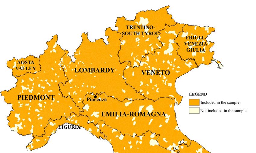
A Geographical coverage of the Istat data in North-
ern Italy
Figure A.1: Geographical coverage of the Istat data in Northern Italy
Notes: Istat released data on the daily number of deaths (deaths from any cause, not
only related to coronavirus) for the period 1st January - 30th March 2020 for 6,866 mu-
nicipalities (87% of the 7.904 total municipalities). In the map, we show the coverage for
Northern Italy with data available for 4,041 municipalities (92% of the 4,383 total mu-
nicipalities).
14B Trajectory balancing and Synthetic weights
Table B.1: Description of control group
Municipality Region Population Traj. bal. weights SCM weights
Piacenza Emilia-Romagna 104,573 NA NA
Alessandria Piedmont 93,636 0 0
Asti Piedmont 76,073 0.04 0
Bergamo Lombardy 122,243 0 0.07
Bolzano Trentino-Alto Adige 107,958 0 0
Busto Arsizio Lombardy 83,874 0 0
Carpi Emilia-Romagna 72,171 0.06 0
Cesena Emilia-Romagna 97,025 0. 0
Cinisello Balsamo Lombardy 76,359 0 0
Como Lombardy 85,469 0 0
Cremona Lombardy 73,040 0.17 0
Cuneo Piedmont 56,032 0.12 0
Faenza Emilia-Romagna 58,831 0 0.09
Ferrara Emilia-Romagna 132,331 0 0
Forlı̀ Emilia-Romagna 117,987 0 0
Gallarate Lombardy 53,517 0 0
Imola Emilia-Romagna 69,870 0 0
La Spezia Liguria 93,297 0 0
Legnano Lombardy 60,638 0 0
Moncalieri Piedmont 57,390 0 0
Monza Lombardy 123,745 0.06 0.46
Novara Piedmont 104,222 0 0.09
Pavia Lombardy 73,217 0 0
Rimini Emilia-Romagna 151,229 0.36 0
Sanremo Liguria 54,637 0 0
Savona Liguria 59,926 0 0
Sesto San Giovanni Lombardy 81,145 0 0
Trento Trentino-Alto Adige 118,872 0.04 0.15
Treviso Veneto 85,667 0.08 0
Udine Friuli-Venezia Giulia 99,042 0 0.14
Varese Lombardy 80,677 0.05 0
Vigevano Lombardy 63,571 0 0
15C Other municipalities
Coronavirus hit many of the municipalities hard in Northern Italy. It is possible
that some of them had signs of coronavirus before 21st February. In this para-
graph, we look at Lodi and Codogno.13 For both of them, we use the same model
specification and the same criterion for selecting the units to include in the donor
pool (i.e., between 50% more or less of the treated municipality population). The
results are reported in Figure C.1. There is no evidence of a positive gap between
the treated and counterfactual trends for Lodi (Panel (a)). Conversely, when look-
ing at Codogno (Panel (b)), there seems to have been an increase in the number of
deaths per 10,000 inhabitants, from late January. However, considering the small
size of the municipality and the small number of deaths, additional evidence is
needed to confirm the potential presence of coronavirus from the end of January.
Trends in number of cumulative deaths per 10,000 inhabitants Trends in number of cumulative deaths per 10,000 inhabitants
Number of cumulative deaths per 10,000 inhabitants
Number of cumulative deaths per 10,000 inhabitants
20 20
15 15
10 10
5 5
0 0
0 10 20 30 40 50 0 10 20 30 40 50
Days (from 1st January 2020) Days (from 1st January 2020)
Lodi Synthetic Lodi Codogno Synthetic Codogno
(a) (b)
Figure C.1: Trends in number of cumulative deaths per 10,000 inhabitants in Lodi,
and Codogno
13
We do not look at Milan, as it is the second-largest Italian city and it would be difficult to find
a valid counterfactual. Besides, in the placebo test we have already shown that Como experienced
an increase in the mortality rate which is about a half of that experienced by Piacenza.
16D Weights leave-one-out
Table D.1: Weights Leave-one-out
Asti Carpi Cremona Cuneo Monza Rimini Trento Treviso Varese
ALESSANDRIA 0.17 0.04 0.04 0.05 0.06 0.02 0.05 0.04 0.04
ASTI NA 0 0 0 0 0 0 0 0
BERGAMO 0 0 0.01 0.01 0.01 0.05 0.02 0.01 0.01
BOLZANO 0 0 0 0 0 0.03 0.01 0 0
BUSTO ARSIZIO 0 0 0 0 0 0 0 0 0
CARPI 0.05 NA 0.09 0.10 0.1 0.08 0.1 0.09 0.1
CESENA 0 0 0 0 0 0 0 0 0
CINISELLO B. 0 0 0 0 0 0 0 0 0
COMO 0.11 0 0.02 0.02 0.04 0.001 0.01 0.02 0.01
CUNEO 0.02 0.03 0.03 NA 0.03 0.01 0.08 0.03 0.03
CREMONA 0.12 0 NA 0 0 0 0 0 0
FAENZA 0 0.01 0.01 0.01 0 0.01 0 0.01 0.01
FERRARA 0 0 0.04 0.04 0.05 0.09 0.01 0.05 0.04
FORLI 0 0.12 0.07 0.07 0.07 0.25 0.03 0.07 0.07
GALLARATE 0.13 0 0.01 0.01 0 0.09 0.02 0.01 0
IMOLA 0 0.01 0.01 0.02 0.01 0.01 0.02 0.02 0.02
LA SPEZIA 0 0 0 0 0 0 0 0 0
LEGNANO 0 0 0 0 0 0.01 0 0 0
MONCALIERI 0 0 0 0 0 0 0 0 0
MONZA 0 0.13 0.10 0.10 NA 0.12 0.11 0.10 0.10
NOVARA 0 0.05 0.05 0.05 0.07 0.05 0.05 0.05 0.05
PAVIA 0 0 0 0 0 0 0 0 0
RIMINI 0.40 0.31 0.30 0.30 0.32 NA 0.39 0.29 0.31
SANREMO 0 0.06 0.07 0.08 0.07 0 0.07 0.07 0.07
SAVONA 0 0 0 0 0 0 0 0 0
SESTO S. GIOV. 0 0 0 0 0 0.01 0 0 0
TRENTO 0.01 0.11 0.11 0.12 0.12 0.24 NA 0.11 0.11
TREVISO 0 0 0.01 0.01 0.01 0.01 0.01 NA 0.01
UDINE 0 0 0 0 0 0 0 0 0
VARESE 0 0 0 0 0 0 0 0 NA
VIGEVANO 0 0.07 0.02 0.02 0.02 0.01 0.01 0.02 0.02
Notes: Column names indicate the municipalities excluded in those iterations.
17References
Abadie, A. (2019): “Using synthetic controls: Feasibility, data requirements, and
methodological aspects,” Journal of Economic Literature.
Abadie, A., A. Diamond, and J. Hainmueller (2010): “Synthetic Control
Methods for Comparative Case Studies: Estimating the Effect of California’s
Tobacco Control Program,” Journal of the American Statistical Association,
105, 493–505.
——— (2015): “Comparative Politics and the Synthetic Control Method,” Amer-
ican Journal of Political Science, 59, 495–510.
Abadie, A. and J. Gardeazabal (2003): “The Economic Costs of Conflict: A
Case Study of the Basque Country,” American Economic Review, 93, 113–132.
Ascani, A., A. Faggian, and S. Montresor (2020): “The geography of
COVID-19 and the structure of local economies: the case of Italy,” mimeo.
Birrell, P. J., L. Wernisch, B. D. M. Tom, L. Held, G. O. Roberts,
R. G. Pebody, and D. De Angelis (2020): “Efficient real-time monitoring
of an emerging influenza pandemic: How feasible?” Ann. Appl. Stat., 14, 74–93.
Buonanno, P., S. Galletta, and M. Puca (2020): “News from the covid-19
epicenter,” Available at SSRN 3567093.
Cereda, D., M. Tirani, F. Rovida, V. Demicheli, M. Ajelli, P. Po-
letti, and S. Merler (2020): “The early phase of the COVID-19 outbreak
in Lombardy, Italy,” arXiv preprint arXiv:2003.09320.
Hazlett, C. and Y. Xu (2018): “Trajectory balancing: A general reweighting
approach to causal inference with time-series cross-sectional data,” Available at
SSRN 3214231.
Peracchi, F. (2020): “The Covid-19 pandemic in Italy,” .
Rothe, C., M. Schunk, P. Sothmann, G. Bretzel, G. Froeschl,
C. Wallrauch, T. Zimmer, V. Thiel, C. Janke, W. Guggemos, et al.
18(2020): “Transmission of 2019-nCoV infection from an asymptomatic contact in
Germany,” New England Journal of Medicine, 382, 970–971.
Setti, L., F. Passarini, G. De Gennaro, P. Barbieri, M. Perrone,
A. Piazzalunga, M. Borelli, J. Palmisani, A. Di Gilio, P. Piscitelli,
and A. Miani (2020): “The Potential role of Particulate Matter in the Spread-
ing of COVID-19 in Northern Italy: First Evidence-based Research Hypotheses,”
medRxiv.
19You can also read