Quantum String Cosmology - Review - MDPI
←
→
Page content transcription
If your browser does not render page correctly, please read the page content below
universe
Review
Quantum String Cosmology
Maurizio Gasperini 1,2

                                           1   Dipartimento di Fisica, Università di Bari, Via G. Amendola 173, 70126 Bari, Italy;
                                               maurizio.gasperini@ba.infn.it
                                           2   Istituto Nazionale di Fisica Nucleare, Sezione di Bari, Via E. Orabona 4, 70125 Bari, Italy

                                           Abstract: We present a short review of possible applications of the Wheeler-De Witt equation to
                                           cosmological models based on the low-energy string effective action, and characterised by an initial
                                           regime of asymptotically flat, low energy, weak coupling evolution. Considering in particular a
                                           class of duality-related (but classically disconnected) background solutions, we shall discuss the
                                           possibility of quantum transitions between the phases of pre-big bang and post-big bang evolution.
                                           We will show that it is possible, in such a context, to represent the birth of our Universe as a quantum
                                           process of tunneling or “anti-tunneling” from an initial state asymptotically approaching the string
                                           perturbative vacuum.

                                           Keywords: string cosmology; quantum cosmology; Wheeler-DeWitt equation

                                           1. Introduction
                                                In the standard cosmological context the Universe is expected to emerge from the big
                                           bang singularity and to evolve initially through a phase of very high curvature and density,
                                           well inside the quantum gravity regime. Quantum cosmology, in that context, turns out
                                           to be a quite appropriate formalism to describe the “birth of our Universe”, possibly in a
                                           state approaching the de Sitter geometric configuration typical of inflation (see, e.g., [1] for
                                 a review).

                                                In the context of string cosmology, in contrast, there are scenarios where the Universe
Citation: Gasperini, M. Quantum
                                           emerges from a state satisfying the postulate of “asymptotic past triviality” [2] (see [3]
String Cosmology. Universe 2021, 7,
                                           for a recent discussion): in that case the initial phase is classical, with a curvature and a
14. https://doi.org/10.3390/
                                           density very small in string (or Planck) units. Even in that case, however, the transition to
universe7010014
                                           the decelerated radiation-dominated evolution, typical of standard cosmology, is expected
                                           to occur after crossing a regime of very high-curvature and strong coupling. The birth of
Received: 26 November 2020
Accepted: 9 January 2021
                                           our Universe, regarded as the beginning of the standard cosmological state, corresponds in
Published: 12 January 2021
                                           that case to the transition (or “bounce”) from the phase of growing to decreasing curvature,
                                           and even in that case can be described by using quantum cosmology methods, like for a
Publisher’s Note: MDPI stays neu-          Universe emerging from an initial singularity.
tral with regard to jurisdictional clai-        There is, however, a crucial difference between a quantum description of the “big
ms in published maps and institutio-       bang” and of the “big bounce”: indeed, the bounce is preceded by a long period of
nal affiliations.                          low-energy, classical evolution, while the standard big bang picture implies that the space-
                                           time dynamics suddenly ends at the singularity, with no classical description at previous
                                           epochs (actually, there are no “previous” epochs, as the time coordinate itself ends at the
                                           singularity). In that context the initial state of the Universe is unknown, and has to be
Copyright: © 2021 by the author. Li-
                                           fixed through some ad hoc prescription: hence, different choices for the initial boundary
censee MDPI, Basel, Switzerland.
                                           conditions are in principle allowed [4–9], leading in general to different quantum pictures
This article is an open access article
                                           for the very early cosmological evolution. Such an approach, based in particular on “no-
distributed under the terms and con-
                                           boundary” initial conditions, has been recently applied also to the ekpyrotic scenario [10],
ditions of the Creative Commons At-
                                           leading to the production of ekpyrotic instantons [11,12]. In the class of string cosmology
tribution (CC BY) license (https://
creativecommons.org/licenses/by/
                                           models considered in this paper, in contrast, the initial state is uniquely determined by
4.0/).
                                           a fixed choice of pre-big bang (or pre-bounce) evolution (see, e.g., [13–17]), which starts

Universe 2021, 7, 14. https://doi.org/10.3390/universe7010014                                                    https://www.mdpi.com/journal/universe
Universe 2021, 7, 14 2 of 14
asymptotically from the string perturbative vacuum and which, in this way, unambiguously
determines the initial “wave function” of the Universe and the subsequent transition
probabilities.
In this paper we report the results of previous works, based on the study of the
Wheeler–De Witt (WDW) equation [18,19] in the “minisuperspace” associated with a
class of cosmological backgrounds compatible with the dynamics the low-energy string
effective action [20–26]. It is possible, in such a context, to obtain a non-vanishing transition
probability between two different geometrical configurations—in particular, from a pre-
big bang to a post-big bang state—even if they are classically disconnected by a space-
time singularity. There is no need, to this purpose, of adding higher-order string-theory
contributions (like α0 and loop corrections) to the WDW equation, except those possibly
encoded into an effective (non-local) dilaton potential (but see [27,28] for high-curvature
contributions to the WDW equation). It will be shown, also, that there are no problems
of operator ordering in the WDW equation, as the ordering is automatically fixed by the
duality symmetry of the effective action. Other possible problems—of conceptual nature
and typical of the WDW approach to quantum cosmology—however, remain, like the the
validity of a probabilistic interpretation of the wave function [29], the existence and the
possible meaning of a semiclassical limit [30], the unambiguous identification of a time-like
coordinate in superspace (see however [23], and see [31] for a recent discussion).
Let us stress that this review is dedicated in particular to string cosmology back-
grounds of the pre-big bang type, and limited to a class of spatially homogeneous geome-
tries. It should be recalled, however, that there are other important works in a quantum
cosmology context which are also directly (or indirectly) related to the string effective
action, and which are applied to more general classes of background geometries not neces-
sarily characterised by spatial Abelian isometries, and not necessarily emerging from the
string vacuum.
We should mention, in particular, the quantum cosmology results for the bosonic
sector of the heterotic string with Bianchi-type IX geometry [32] and Bianchi class A ge-
ometry [33]; solutions for the WDW wave function with quadratic and cubic curvature
corrections [34] (typical of f ( R) models of gravity), describing a phase of conventional
inflation; two-dimensional models of dilaton quantum cosmology and their supersymmet-
ric extension [35]; WDW equation for a class of scalar-tensor theories of gravity with a
generalised form of scale-factor duality invariance [36,37]. We think that discussing those
(and related) works should deserve by itself a separate review paper.
This paper is organized as follows. In Section 2 we present the explicit form of the
WDW equation following from the low-energy string effective action, for homogeneous
backgrounds with d Abelian spatial isometries, and show that it is free from operator-
ordering ambiguities thanks to its intrinsic O(d, d) symmetry. In Section 3, working in
the simple two-dimensional minisuperspace associated with a class of exact gravi-dilaton
solutions of the string cosmology equations, we discuss the scattering of the WDW wave
function induced by the presence of a generic dilaton potential. In Section 4 we show that
an appropriate quantum reflection of the wave function can be physically interpreted as
representing the birth of our Universe as a process of tunnelling from the string perturbative
vacuum. Similarly, in Section 5, we show that the parametric amplification of the WDW
wave function can describe the birth of our Universe as a process of “anti-tunnelling” from
the string perturbative vacuum. Section 6 is finally devoted to a few conclusive remarks.
2. The Wheeler-De Witt Equation for the Low-Energy String Effective Action
In a quantum cosmology context the Universe is described by a wave function evolving
in the so-called superspace and governed by the WDW equation [18,19], in much the
same way as in ordinary quantum mechanics a particle is described by a wave function
evolving in Hilbert space [38], governed by the Schrodinger equation. Each point of
superspace corresponds to a possible geometric configuration of the space-like sections of
our cosmological space-time, and the propagation of the WDW wave function through thisUniverse 2021, 7, 14 3 of 14
manifold describes the quantum dynamics of the cosmological geometry (thus providing,
in particular, the transition probabilities between different geometric states).
The WDW equation, which implements the Hamiltonian constraint H = 0 in the
superspace of the chosen cosmological scenario, has to be obtained, in our context, from
the appropriate string effective action. Let us consider, to this purpose, the low-energy, tree-
level, (d + 1)-dimensional (super)string effective action, which can be written as [39–41]
1 1
Z
d +1 −φ µ µνα
S = − d −1 d x −g e R + ∂µ φ∂ φ − Hµνα H +V , (1)
p
2λs 12
where φ is the dilaton [42], Hµνα = ∂µ Bνα + ∂ν Bαµ + ∂α Bµν is the field strength of the
NS-NS two form Bµν = − Bνµ (also called Kalb-Ramond axion), and λs ≡ (α0 )1/2 is the
fundamental string length parameter. We have also added a possible non-trivial dilaton
potential V (φ).
For the purpose of this paper it will be enough to consider a class of homogeneous
backgrounds with d Abelian spatial isometries and spatial sections of finite volume, i.e.,
√
( dd x − g)t=const < ∞. In the synchronous frame where g00 = 1, g0i = 0 = B0i , and
R
where the fields are independent of all space-like coordinates xi (i, j = 1, .., d), the above
action can then be rewritten as follows [43,44]:
1
λs
Z
S = dt L(φ, M), L = − e−φ (φ̇)2 + Tr Ṁ ( M−1 )˙ + V . (2)
2 8
Here a dot denotes differentiation with respect to the cosmic time t, and φ is the so-called
“shifted” dilaton field,
φ = φ − ln − g, (3)
p
where we have absorbed into φ the constant shift − ln(λ− d dd x ). Finally, M is the
R
s
2d × 2d matrix −1
G − G −1 B
M= , (4)
BG −1 G − BG −1 B
where G and B are, respectively, d × d matrix representations of the spatial part of the
metric (gij ) and of the antisymmetric tensor (Bij ). For constant V, or for V = V (φ), the
above action (2) is invariant under global O(d, d) transformations [43,44] that leave the
shifted dilaton invariant, and that are parametrized in general by a constant matrix Ω
such that
φ → φ, M → Ω T MΩ, (5)
where Ω satisfies
0 I
T
Ω ηΩ = η, η= , (6)
I 0
and I is the d-dimensional identity matrix. It can be easily checked that, in the particular
case in which B = 0 and Ω coincides with η, Equation (5) reproduces the well-known
transformation of scale-factor duality symmetry [45,46].
From the effective Lagrangian (2) we can now obtain the (dimensionless) canoni-
cal momenta
δL δL λs
Πφ = = −λs φ̇e−φ , ΠM = = e−φ M−1 ṀM−1 , (7)
δφ̇ δ Ṁ 8
and the associated classical Hamiltonian:
eφ h i
H= −Π2φ + 8Tr( M Π M M Π M ) + λ2s Ve−2φ . (8)
2λs
The corresponding WDW equation, implementing in superspace the Hamiltonian con-
straint H = 0 through the differential operator representation Πφ = ±iδ/δφ, Π M =Universe 2021, 7, 14 4 of 14
±iδ/δM, would seem thus to be affected by the usual problems of operator ordering, since
[ M, Π M ] 6= 0.
The problem disappears, however, if we use the O(d, d) covariance of the action (2),
and the symmetry properties of the axion-graviton field represented by the matrix (4),
which satisfies the identity Mη = η M−1 . Thanks to this property, in fact, we can identi-
cally rewrite the axion-graviton part of the kinetic term appearing in the Lagrangian (2)
as follows:
Tr Ṁ ( M−1 )˙ = Tr Ṁη Ṁη . (9)
The corresponding canonical momentum becomes
λs −φ
ΠM = − e η Ṁη, (10)
8
and the associated Hamiltonian
eφ h i
H= −Π2φ − 8Tr(η Π M η Π M ) + λ2s Ve−2φ (11)
2λs
has a flat metric in momentum space, and leads to a WDW equation
δ2
" #
δ δ 2 −2φ
2
+ 8Tr η η + λs Ve Ψ(φ, M) = 0 (12)
δφ δM δM
which is manifestly free from problems of operator ordering.
Finally, it may be interesting to note that the quantum ordering imposed by the dualiy
symmetry of the effective action is exactly equivalent to the order fixed by the condition of
reparametrization invariance in superspace.
To check this point let us consider a simple spatially isotropic background, with Bij = 0
and scale factor a(t), so that Gij = − a2 (t)δij . The effective Lagrangian (2) becomes
ȧ2
λs −φ 2
L(φ, a) = − e φ̇ − d 2 + V , (13)
2 a
with associated canonical momenta
δL δL ȧ
Πφ = = −λs φ̇e−φ , Πa = = λs d 2 e−φ , (14)
δφ̇ δ ȧ a
and Hamiltonian constraint:
a2 2
2λs e−φ H = −Π2φ + Π + λ2s Ve−2φ = 0. (15)
d a
The differential implementation of this constraint in terms of the operators Πφ → ±i∂/∂φ,
Π a → ±i∂/∂a has to be ordered, because [ a, Π a ] 6= 0. It follows that in general, for the
kinetic part of the Hamiltonian Hk = −Π2φ + a2 Π2a /d, we have the following differen-
tial representation
∂ a2 ∂2 a ∂
Hk = 2
− 2
−e , (16)
∂φ d ∂a d ∂a
where e is a numerical parameter depending on the imposed ordering. However, if
we perform a scale-factor duality transformation φ → φ, a → e a = a−1 (which exactly
corresponds to the class of transformations (5) for the particular class of backgrounds that
we are considering), we find
2 ∂
a ) + ( e − 1) e
Hk ( a) = Hk (e a . (17)
d a
∂eUniverse 2021, 7, 14 5 of 14
The duality invariance of the Hamiltonian thus requires e = 1 (which, by the way, is
also the value of e that we have to insert into Equation (16) to be in agreement with
the general result (12) if we consider the particular class of geometries with B = 0 and
G = − a2 I). See also [36,37] for the WDW equation with a generalised form of scale-factor
duality symmetry.
Let us now consider the kinetic part of the Hamiltonian operator (15), which is given
as a quadratic form in the canonical momenta Π A = (Πφ , Π a ), written in a 2-dimensional
minisuperspace with a non-trivial metric γ AB and coordinates x A = (φ, a), such that:
a2 d
Hk = −Π2φ + Π2a ≡ γ AB Π A Π B , γ AB (φ, a) = diag −1, 2 . (18)
d a
If we impose on the differential representation of the Hamiltonian constraint the condition
of general covariance with respect to the given minisuperspace geometry [47], we obtain
1 √ ∂ a2 ∂2 a ∂
Hk = −γ AB ∇ A ∇ B = − √ ∂ A ( −γγ AB ∂ B ) ≡ 2
− 2
− , (19)
−γ ∂φ d ∂a d ∂a
and this result exactly reproduces the differential operator (16) with e = 1. The duality
symmetry of the action, and the requirement of reparametrisation invariance in superspace,
are thus equivalent to select just the same ordering prescription, as previously anticipated.
3. Quantum Scattering of the Wheeler-De Witt Wave Function in Minisuperspace
For an elementary discussion of this topic, and for the particular applications we
have in mind—namely, a quantum description of the “birth” of our present cosmological
state from the string perturbative vacuum—we shall consider the homogeneous, isotropic
and spatially flat class of (d + 1)-dimensional backgrounds already introduced in the
previous section, with Bµν = 0, g00 = 1 and scale factor a(t). We shall thus work in a
two-dimensional
√ minisuperspace, spanned by the convenient coordinates (φ, β) where
β = d ln a. With such variables the effective Lagrangian (2) takes the form
e−φ h 2 i
L( β, φ) = −λs φ̇ − β̇2 + V ( β, φ) , (20)
2
and the momenta, canonically conjugate to the coordinates φ, β, are given by
δL δL
Πφ = = −λs φ̇e−φ , Πβ = = λs β̇ e−φ . (21)
δφ̇ δ β̇
The Hamiltonian constraint (15) becomes
− Π2φ + Π2β + λ2s V ( β, φ) e−2 φ = 0, (22)
corresponding to an effective WDW equation
h i
∂2φ − ∂2β + λ2s V ( β, φ) e−2φ Ψ( β, φ) = 0. (23)
For V = 0 we have the free D’Alembert equation, and the general solution can be written
in terms of plane waves as
Ψ( β, φ) = ψβ± ψφ± ∼ e∓ikβ e∓ikφ . (24)
Here k > 0, and ψβ± , ψφ± are free momentum eigenstates, satisfying the eigenvalue equations
Π β ψβ± = ±k ψβ± , Πφ ψφ± = ±k ψφ± . (25)Universe 2021, 7, 14 6 of 14
Let us now recall that, for V = 0, the equations following from the effective La-
grangian (20) admit a class of exact solution describing four (physically different) cosmo-
logical phases, two expanding and two contracting, parametrized by [13,15–17]:
√
a(t) ∼ (∓t)∓1/ d
, φ(t) ∼ − ln(∓t), (26)
They are defined on the disconnected time ranges [−∞, 0] and [0, +∞], and are related
by duality transformations a → a−1 , φ → φ and time-reversal transformation, t → −t.
They may represent the four asymptotic branches of the low-energy string cosmology
solutions even in the presence of a non-vanishing dilaton potential, provided the effective
contribution of the potential is localized in a region of finite extension of the (φ, β) plane,
and goes (rapidly enough) to zero as φ, β → ±∞.
The above solutions satisfy the condition
√ ȧ
φ̇ = ± d = ± β̇, (27)
a
so that, according to the definitions (21), they correspond to configurations with canonical
momenta related by Π β = ±Πφ . By recalling that the phase of (expanding or contracting)
pre-big bang evolution is characterized by growing curvature and growing dilaton [15,16]
(namely, φ̇ > 0, Πφ < 0), while the curvature and the dilaton are decreasing in the
(expanding or contracting) post-big bang phase (where φ̇ < 0, Πφ > 0), we can conclude,
according to Equations (21), (25), that the classical solutions (26) of the string cosmology
equations admit the following plane-wave representation in minisuperspace in terms of
ψβ± , ψφ± :
• expansion −→ β̇ > 0 −→ ψβ+ ,
• contraction −→ β̇ < 0 −→ ψβ− ,
• pre-big bang (growing dilaton) −→ φ̇ > 0 −→ ψφ− ,
• post-big bang (decreasing dilaton) −→ φ̇ < 0 −→ ψφ+ .
Let us now impose, as our physical boundary condition, that the initial state of our
Universe describes a phase of expanding pre-big bang evolution, asymptotically emerging
from the string perturbative vacuum (identified with the limit β → −∞, φ → −∞). It
follows that the initial state Ψin must represent a configuration with β̇ > 0 and φ̇ > 0,
namely a state with positive eigenvalue of Π β and negative (opposite) eigenvalue of Πφ ,
i.e., Ψin ∼ ψβ+ ψφ− .
In such a context, a quantum transition from the pre- to the post-big bang regime can
be described as a process of scattering of the initial wave function induced by the presence
of some appropriate dilaton potential, which we shall assume to have non-negligible
dynamical effects only in a finite region localized around the origin of the minusuperspace
spanned by the (φ, β) coordinates. In other words, we shall assume that the contributions
of V (φ) to the WDW equation tend to disappear not only in the initial but also in the final
asymptotic regime where β → +∞, φ → +∞. As a consequence, also the final asymptotic
configuration Ψout , emerging from the scattering process, can be represented in terms of
the free momentum eigenstates ψβ± and ψφ± .
However, unlike the initial state fixed by the chosen boundary conditions—and
selected to represent a configuration with Π β > 0 and Πφ < 0—the final state is not
constrained by such a restriction and can describe in general different configurations. In
particular, the scattering process may lead to configurations asymptotically described by
a wave function Ψout which is a superposition of different momentum eigenstates: for
instance, waves with the same Π β > 0 and opposite values of Πφ , i.e., Ψout ∼ ψβ+ ψφ± (see
Figure 1, cases (a) and (b)); or waves with the same Πφ < 0 and opposite values of Π β , i.e.,
Ψout ∼ ψφ− ψβ± (see Figure 1, cases (c) and (d)).Universe 2021, 7, 14 7 of 14
Version January 4, 2021 submitted to Universe 7 of 15
t x
+ + + _ + _
x t
+ _ + _ + +
(a) (b)
x t
+ _ _ _ + _
t x
+ _ _ _ + _
(c) (d)
Fourdifferent
Figure1.1. Four
Figure different classes
classes of
of scattering
scattering processes
processes for
for the
the incoming
incoming wave
wavefunction
functiondescribing
describingaa
phase of expanding pre-big bang evolution, asymptotically emerging from the string
phase of expanding pre-big bang evolution, asymptotically emerging from the string perturbative perturbative
vacuum(straight,
vacuum (straight, solid
solid line).
line). The
The outgoing
outgoing state
state is
is represented
represented byby aa mixture
mixtureof eigenfunctionsofofΠΠββ
ofeigenfunctions
andΠΠφwith
and withpositive
positiveand
andnegative
negativeeigenvalues.
eigenvalues. See the main text for a detailed explanation of the
φ
four different cases (a–d) illustrated in this figure.
138 restrictionItand may canbedescribe
interestingin general
to note different
that those configurations. In particular,
different configurations maythebescattering
interpreted process
139 may lead to configurations
as different possible asymptotically
“decay channels” described
of the by a wave
string function Ψvacuum
perturbative out which[24].
is a superposition
Also, it
140 of different eigenstates: for instance, waves with the same Π
should be stressed (as clearly illustrated in Figure 1) that one of the two components ofvalues
momentum β > 0 and opposite
+ ±
141 of Πφthe Ψout ∼ ψwave
, i.e.outgoing β ψφ (see Fig. Ψ
function 1,out
cases
must and (bcorrespond
( a)always )); or wavestowith the the same Πφ 0 and Πφ < 0, represented
state(dwith
+ −
143 Itbymay
ψβ ψ be . However, the “reflected” part of the wave function may have different physical
φ interesting to note that those different configurations may be interpreted as different
144 interpretations,
possible “decay channels" alsoof depending on the chosen
the string perturbative identification
vacuum of it
[24]. Also, the time-like
should coordinate
be stressed (as clearly
145 illustrated in Fig. 1) that one of the two components of the outgoing wave function Ψout must(b)
in minisuperspace [23,25]: the β axis for the cases (a) and (d), the φ axis for the case always
146 and (c).
correspond to the “transmitted" part of the incident wave Ψin , namely must correspond to a state with
Π β > 0 and It Π
turns out that only the cases + − (a) and (c) of Figure 1 represent a true process of
147
φ < 0, represented by ψβ ψ . However, the “reflected" part of the wave function may
reflection of the incident wave alongφa spacelike coordinate (the axes φ and β, respectively).
148 have different physical interpretations, also depending on the chosen identification of the time-like
In case (a), in particular, the evolution along β is monotonic, the Universe always keeps
149 coordinate in minisuperspace [23,25]: the β axis for the cases ( a) and (d), the φ axis for the case (b)
expanding, and the incident wave Ψin is partially transmitted towards the pre-big bang
150 and (c).
singularity (with unbounded growth of the curvature and of the dilaton, β → +∞, φ →
151 It
+turns
∞), and out that only
partially the cases
reflected ) and (c)the
back( atowards of expanding,
Fig. 1 represent a true process
low-energy, post-bigof reflection
bang regimeof the
152 incident
(β → wave
+∞,along
φ → a−spacelike
∞). As we coordinate
shall show (the
in axes φ and
Section β, respectively).
4, this type of quantum In case ( a), in particular,
reflection can
153 the evolution along β is monotonic, the Universe always keeps expanding,
also be interpreted as a process of “tunnelling” from the string perturbative vacuum. and the incident waveUniverse 2021, 7, 14 8 of 14
The cases (b) and (d) of Figure 1 are qualitatively different, as the final state is a super-
position of modes of positive and negative frequency with respect to the chosen timelike
coordinate (the axes φ and β, respectively). Namely, Ψout is a superposition of positive and
negative energy eigenstates, and this represents a quantum process of “parametric amplifi-
cation” of the wave function [48,49] or, in the language of third quantization [50–54]—i.e.,
second quantization of the WDW wave function—a process of “Bogoliubov mixing” of
the energy modes (see, e.g., [55,56]), associated with the production of “pairs of universes”
from the vacuum. For that process, the mode “moving backwards” with respect to the
chosen time coordinate has to be “reinterpreted”: as an anti-particle in the usual quantum
field theory context, as an “anti-universe” in a quantum cosmology context.
Such a re-interpretation principle produces, as usual, states of positive energy and
opposite momentum. It turns out, in particular, that the case (d) of Figure 1 describes—after
the correct re-interpretation—the production of universe/anti-universe pairs in which both
members of the pair have positive energy and positive momentum along the β axis. Hence,
they are both expanding: one falls inside the pre-big bang singularity (φ → +∞), but the
other expands towards the low-energy post-big bang regime (φ → −∞). As we shall show
in Section 5, this quantum effect of pair production can also be interpreted as a process of
“anti-tunnelling” from the string perturbative vacuum.
4. Birth of the Universe as a Tunnelling from the String Perturbative Vacuum
To illustrate the process of quantum transition from the pre- to the post-big bang
regime as a wave reflection in superspace we shall consider here the simplest (almost trivial)
case of constant dilaton potential, V = V0 = const ( see also [37], and see, e.g., [20] for more
general dynamical configurations). With this potential the classical background solutions
for the cosmological equations of the effective Lagrangian (20) are well known [57], and
can be written as
h p i∓1/√d h p i
a(t) = a0 tanh ∓ V0 t/2 , φ = φ0 − ln sinh ∓ V0 t , (28)
where a0 and φ0 are integration constants.
These solutions have two branches, of the pre-big bang type (φ̇ > 0) and post-big bang
type (φ̇ < 0), defined respectively over the disconnected time ranges t < 0 and t > 0, and
classically separated by a singularity of the curvature and of the effective string coupling
(exp φ) at t = 0. For t → ±∞ they approach, asymptotically, the free vacuum solution (26)
obtained for V = 0. It is important to note, also, that each branch of the above solution
can describe either expanding or contracting geometric configurations, which are both
characterized by a constant canonical momentum along the β axis, given (according to
Equation (21)), by
Π β = λs β̇ e−φ = ±k, k = λs V0 e−φ0 .
p
(29)
Let us now apply the WDW Equation (23) to compute the (classically forbidden)
probability of transition from the pre- to the post-big bang branches of the solution (28).
We are interested, in particular, in the transition between expanding configurations, and
we shall thus consider the quantum process described by the case (a) of Figure 1, with a
wave function monotonically evolving along the positive direction of the β axis (also in
agreement with the role of time-like coordinate asssigned to β). In that case β̇ > 0, and
the conserved canonical momentum (29) is positive, Π β > 0. By imposing momentum
conservation as a differential condition on the wave function,
Π β Ψk ( β, φ) = i∂ β Ψk ( β, φ) = k Ψk ( β, φ), (30)
we can then separate the variables in the solution of the WDW Equation (23), and we obtain
Ψ( β, φ) = e−ikβ ψk (φ), ∂2φ + k2 + λ2s V0 e−2φ ψk (φ) = 0. (31)Universe 2021, 7, 14 9 of 14
The general solution of the above equation can now be written as a linear combination
of Bessel√ functions [58], AJν (z) + BJ−ν (z), of index ν = ik and argument
z = λs V0 exp(−φ). Consistently with the chosen boundary conditions for the pro-
cess illustrated in case (a) of Figure 1 (namely, with the choice of an initial wave function
asymptotically incoming from the string perturbative vacuum), we have now to impose
that there are only right-moving waves (along φ) approaching the high-energy region and
the final singularity in the limit β → +∞, φ → +∞. Namely, waves of the type ψφ− —see
Equations (24) and (25)—representing a state with φ̇ > 0 and Πφ < 0. By using the small
argument limit of the Bessel functions [58],
p
lim J±ik λs V0 e−φ ∼ e∓ikφ , (32)
φ→+∞
we can then eliminate the Jν (z) component and uniquely fix the WDW solution (modulo
an arbitrary normalization factor Nk ) as follows:
p
Ψk ( β, φ) = Nk J−ik λs V0 e−φ e−ikβ . (33)
Let us now consider the wave content of this solution in the opposite, low-energy
limit φ → −∞, where the large argument limit of the Bessel functions gives [58]
Nk e−ikβ h −i(z−π/4) kπ/2 i (z−π/4) −kπ/2
i
lim Ψk ( β, φ) = e e + e e
φ→−∞ (2πz)1/2
≡ Ψ− +
k ( β, φ ) + Ψk ( β, φ ), (34)
and where the two wave components Ψ− +
k and Ψk are asymptotically eigenstates of Πφ with
negative and positive eigenvalues, respectively. Hence, we find in this limit a superposition
of right-moving and left-moving modes (along φ), representing, respectively, the initial,
pre-big bang incoming state Ψ− k (with Πφ < 0, i.e., growing dilaton), and the final, post-big
+
bang reflected component Ψk (with Πφ > 0, i.e., decreasing dilaton). Starting from an
initial pre-big bang configuration, we can then obtain a finite probability for the transition
to the “dual” post-big bang regime, represented as a reflection of the wave function in
minisuperspace, with reflection coefficient
2
Ψ+
k ( β, φ )
Rk = 2
= e−2πk . (35)
Ψ−
k ( β, φ )
The probability for this quantum process is in general nonzero, even if the corresponding
transition is classically forbidden.
It may be interesting to evaluate Rk in terms of the string-scale variables, for a region
of d-dimensional space of given proper volume Ωs . By computing
√ the constant
√ momentum
k of Equation (29) at the string epoch ts , when β̇(ts ) = d( ȧ/a)(ts ) ' dλ− 1 , and using
s
the definition (3) of φ, we find
( √ )
2π d Ωs
Rk ∼ exp − , (36)
gs2 λds
where the proper spatial volume is given by Ωs = ad (ts ) dd x, and where gs = exp(φs /2)
R
is the effective value of the string coupling when the dilaton has the value φs ≡ φ(ts ). Note
that, for values of the coupling gs ∼ 1, the above probability is of order one for the formation
of spacelike “bubbles” of unit size (or smaller) in string units. In general, the probability
has a typical “instanton-like” dependence on the coupling constant, Rk ∼ exp( gs−2 ).
It may be observed, finally, that an exponential dependence of the transition proba-
bility is also typical of tunnelling processes (induced by the presence of a cosmologicalUniverse 2021, 7, 14 10 of 14
constant Λ) occurring in the context of standard quantum cosmology, where the tunnelling
probability can be estimated as [6,29,59,60]
( )
4
P ∼ exp − 2 (37)
λP Λ
(λ P is the Planck length). That scenario is different because, in that case, the Universe
emerges from the quantum era in a classical inflationary configuration, while, in the string
scenario, the Universe is expected to exit (and not to enter) the phase of inflation thanks to
quantum cosmology effects.
In spite of such important differences, it turns out that the string cosmology result (36)
is formally very similar to the result concerning the probability that the birth of our
Universe may be described as a quantum process of “tunneling from nothing” [6,29,59,60].
The explanation of this formal coincidence is simple, and based on the fact that the choice
of the string perturbative vacuum as initial boundary condition implies—as previously
stressed—that the are only outgoing (right-moving) waves approaching the singularity
at φ → +∞. This is exactly equivalent to imposing tunneling boundary conditions, that
select “... only outgoing modes at the singular space-time boundary” [29,60]. In this sense, the
process illustrated in this Section can also be interpreted as a tunneling process, not “from
nothing” but “from the string perturbative vacuum”.
5. Birth of the Universe as Anti-Tunnelling from the String Perturbative Vacuum
In this Section we shall illustrate the possible transition from the pre- to the post-big
bang regime as a process of parametric amplification of the WDW wave function, also
equivalent—as previously stressed—to a quantum process of pair production from the
vacuum. We shall consider, in particular, an example in which both the initial and final
configurations are expanding, like in the case (d) of Figure 1.
What we need, to this purpose, is a WDW equation with the appropriate dilaton
potential, able to produce an outgoing configuration which is a superposition of states
with positive and negative eigenvalues of the momentum Π β (see Figure 1). Since we are
starting from an initial expanding (pre-big bang) regime, it follows that the contribution
of the potential has to break the traslational invariance of the effective Hamiltonian (22)
along the β axis (i.e., [Π β , H ] 6= 0), otherwise the final configuration described in case (d)
of Figure 1 would be forbidden by momentum conservation.
We shall work here with the simple two-loop dilaton potential already introduced
in [26], possibly induced by an effective cosmological constant Λ > 0, appropriately
suppressed in the low-energy, classical regime, and given explicitly by
√
V ( β, φ) = Λ θ (− β) e2φ = Λ θ (− β) e2φ+2 dβ
. (38)
The Heaviside step function θ has been inserted to mimic an efficient damping of the
potential outside the interaction region (in particular, in the large radius limit β → +∞ of
the expanding post-bb configuration). The explicit form and mechanism of the damping,
however, is not at all a crucial ingredient of our discussion, and other, different forms of
damping would be equally appropriate.
With the given potential (38) the effective Hamiltonian is no longer translational
invariant along the β direction, but we still have [Πφ , H ] = 0, so that we can conveniently
separate the variables in the WDW Equation (23) by factorizing the eigenstates (25) of the
canonical momentum Πφ , and we are lead to
h √ i
Ψ( β, φ) = eikφ ψk ( β), ∂2β + k2 − λ2s Λ θ (− β) e2 dβ
ψk ( β) = 0. (39)
The above WDW equation can now be exactly solved by separately considering the two
ranges of the “temporal coordinate” β, namely β < 0 and β > 0.Universe 2021, 7, 14 11 of 14
For β < 0 the contribution of the potential is non vanishing, and the general solu-
√
tion is a linear combination of Bessel functions Jµ (σ) and J−µ (σ ), of index µ = ik/ d
√ √
and argument σ = iλs Λ/d e dβ . As before, we have to impose our initial boundary
conditions requiring that, in the limit β → −∞, the solution may asymptotically represent
a low-energy pre-big bang configuration with Π β = −Πφ = k, namely (according to
Equations (24) and (25)):
lim Ψ( β, φ) ∼ ψβ+ ψφ− ∼ eikφ−ikβ . (40)
β→−∞
By using the small argument limit (32), and imposing the above condition, we can then
uniquely fix (modulo a normalization factor Nk ) the solution of the WDW Equation (39),
for β < 0, as follows:
√ √
Ψk ( β, φ) = eikφ Nk J−ik/√d iλs Λ/d e dβ , β < 0. (41)
In the complementary regime β > 0 the potential (38) is exactly vanishing, and the
general outgoing solution is a linear superposition of eigenstates of Π β with positive and
negative eigenvalues, represented by the frequency modes ψβ± of Equations (24) and (25).
We can then write
h i
Ψk ( β, φ) = eikφ A+ (k )e−ikβ + A− (k )eikβ , β > 0, (42)
and the numerical coefficients A± (k) can be fixed by the two matching conditions imposing
the continuity of Ψk and ∂ β Ψk at β = 0.
Let us now recall that the so-called Bogoliubov coefficients |c± (k)|2 = | A± (k)|2 /| Nk |2 ,
determining the mixing of positive and negative energy modes in the asymptotic outgoing
solution [55,56], also play the role of destruction and creation operators in the context
of the third quantization formalism [50–54], thus controlling the “number of universes”
nk = |c− (k)|2 produced from the vacuum, for each mode k. It turns out, in particular,
that such a transition from the initial vacuum to the final standard regime, represented
as a quantum scattering of the initial wave function, is an efficient process only when the
final wave function is not damped but, on the contrary, turns out to be “parametrically
amplified” by the interaction with the effective potential barrier [48,49]. This is indeed
what happens for the solutions √ of our WDW Equation (39), provided the dilaton potential
satisfies the condition k < λs Λ [26] (as can be checked by an explicit computation of our
coefficients A± (k )).
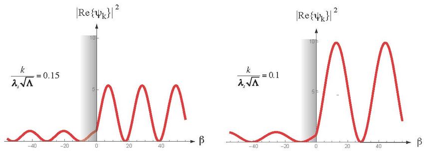
In order to illustrate this effect we have numerically integrated Equation (39),
with the boundary conditions (40), for d = 3 spatial dimensions. The results are
shown in Figure 2, where we have plotted the evolution in superspace of the real part of
the WDW wave function, for different values of k (the behavior of the imaginary part is
qualitatively similar). We have used units where λ2s Λ = 1, so that the effective potential
barrier of Equation (39) is non-negligible only for very small (negative) values of β (the
grey shaded region of Figure 2). Also, we have imposed on all modes the same formal
normalization |Ψk |2 = 1 at β → −∞, to emphasize that the amplification is more effective
at lower frequency.Universe 2021, 7, 14 12 of 14
Figure 2. Evolution in superspace of the Wheeler–De Witt (WDW) solution which illustrates the
anti-tunnelling effect produced by the effective potential barrier (grey shaded region) due to the
dilaton potential (38). The wave function is not damped but parametrically amplified provided
√
k < λs Λ, and the effect is larger for smaller k.
Concerning this last√ point, we can find an interesting (and reasonable) interpretation
of the condition k < λs Λ by considering the realistic case of a transition process occurring
at the string scale, with β̇ ∼ λs , with coupling constant gs , and for a spatial region of proper
volume Ωs . In that case, by using the result (36) for the momentum k expressed in terms of
string-scale variables, we can write the condition of efficient parametric amplification in
the following form: √
k ∼ gs−2 (Ωs /λds ) <
∼ λs Λ. (43)
It implies that the birth of our present, expanding, post-big bang phase can be efficiently
described as a process of anti-tunnelling—or, in other words, as a forced production of
pairs of universes—from the string perturbative vacuum, in the following cases: initial
configurations of small enough volume in string units, and/or large enough coupling gs ,
and/or large enough cosmological constant in string units. Quite similar conclusions were
obtained also in the case discussed in the previous section.
In view of the above results, we may conclude that, for an appropriate initial con-
figuration, and if triggered by the appropriate dilaton potential, the decay of the initial
string perturbative vacuum can efficiently proceed via parametric amplification of the
WDW wave function in superspace, and can be described as a forced production of pairs
of universes from the quantum fluctuations. One member of the pair disappears into the
pre-big bang singularity, the other bounces back towards the low-energy regime. The
resulting effect is a net flux of universes that may escape to infinity in the post-big bang
Version January 4, 2021 submitted to Universe 13 of 15
regime (as qualitatively illustrated in Figure 3), with a process which can describe the birth
of our Universe as “anti-tunnelling from the string perturbative vacuum”.
Figure 3. Birth of
Figure 3.the universe
Birth represented
of the universeasrepresented
an anti-tunneling (parametric
as an amplification)
anti-tunneling effect of the
(parametric amplification) effect of
wave function in superspace, or – in the language of third quantization – as a process of pair production
the wave function in superspace, or—in the language of third quantization—as a process of pair
from the string perturbative vacuum.
production from the string perturbative vacuum.
261 Funding: This research received no external funding.
262 Acknowledgments: It is a great pleasure to thank all colleagues and friends who collaborated and made many
263 important contributions to the original research articles reported in this paper. Let me mention, in particular
264 (and in alphabetical order): Alessandra Buonanno, Marco Cavaglià, Michele Maggiore, Jnan Maharana, Carlo
265 Ungarelli, Gabriele Veneziano. This work is supported in part by INFN under the program TAsP (Theoretical
266 Astroparticle Physics), and by the research grant number 2017W4HA7S (NAT-NET: Neutrino and Astroparticle Theory
267 Network), under the program PRIN 2017, funded by MUR.Universe 2021, 7, 14 13 of 14
6. Conclusions
The quantum cosmology scenarios reported in this review are based on the low-energy,
tree-level string effective action, which is physically appropriate to describe early enough
and late enough cosmological phases, approaching, respectively, the initial perturbative
vacuum and the present cosmological epoch.
Such an action cannot used to classically describe the high-curvature, strong coupling
regime without the inclusion of higher-order corrections. However, when at least some
of these corrections and of possible non-perturbative effects are accounted for by an
appropriate dilaton potential, the WDW equation obtained from the low-energy action
action permits a quantum analysis of the background evolution, and points out new
possible interesting ways for a Universe born from the string vacuum to reach more
standard configurations, and evolve towards the present cosmological regime. In such a
context, the possible (future) detection of a stochastic background of cosmic gravitons with
the typical imprints of the pre-big bang dynamics (see, e.g., [61]) might thus represent also
an “indirect” indication that some quantum cosmology mechanism has been effective to
trigger the transition to the cosmological state in which we are living.
Funding: This research received no external funding.
Institutional Review Board Statement: Not applicable.
Informed Consent Statement: Not applicable.
Data Availability Statement: Not applicable.
Acknowledgments: It is a great pleasure to thank all colleagues and friends who collaborated
and made many important contributions to the original research articles reported in this paper.
Let me mention, in particular (and in alphabetical order): Alessandra Buonanno, Marco Cavaglià,
Michele Maggiore, Jnan Maharana, Carlo Ungarelli, Gabriele Veneziano. This work is supported in
part by INFN under the program TAsP (Theoretical Astroparticle Physics), and by the research grant
number 2017W4HA7S (NAT-NET: Neutrino and Astroparticle Theory Network), under the program
PRIN 2017, funded by MUR.
Conflicts of Interest: The author declares no conflict of interest.
Abbreviations
The following abbreviations are used in this manuscript:
WDW Wheeler-De Witt equation
References
1. Vilenkin, A. Predictions from Quantum Cosmology. In Contribution to the 4th Course of the International School of Astrophysics D,
Proceedings of the String Gravity and Physics at the Planck Energy Scale, A NATO Advanced Study Institute, Erice, Italy, 8–19 September
1995; NATO: Brussels, Belgium, 1996; Volume 476, pp. 345–367.
2. Buonanno, A.; Damour, T.; Veneziano, G. Pre–big bang bubbles from the gravitational instability of generic string vacua.
Nucl. Phys. 1999, B543, 275.
3. Gasperini, M. On the initial regime of pre-big bang cosmology. J. Cosmol. Astropart. Phys. 2017, 9, 001.
4. Hartle, J.B.; Hawking, S.W. Wave Function of the Universe. Phys. Rev. 1983, 28, 2960.
5. Hawking, S.W. The Quantum State of the Universe. Nucl. Phys. 1984, 239, 257.
6. Vilenkin, A. Quantum Creation of Universes. Phys. Rev. 1984, 30, 509.
7. Linde, A.D. Quantum creation of an inflationary universe. Sov. Phys. JETP 1984, 60, 211.
8. Zeldovich, Y.; Starobinski, A.A. Quantum creation of a universe in a nontrivial topology. Sov. Astron. Lett. 1984, 10, 135.
9. Rubakov, V.A. Quantum Mechanics in the Tunneling Universe. Phys. Lett. 1984, B148, 280.
10. Khoury, J.; Ovrut, B.A.; Steinhardt, P.J.; Turok, N. The Ekpyrotic universe: Colliding branes and the origin of the hot big bang.
Phys. Rev. 2001, 64, 123522.
11. Lehners, J.-L. Classical Inflationary and Ekpyrotic Universes in the No-Boundary Wavefunction. Phys. Rev. 2015, 91, 083525.
12. Lehners, J.-L. New ekpyrotic quantum cosmology. Phys. Lett. 2015, 750, 242.
13. Gasperini, M.; Veneziano, G. Pre-big bang in string cosmology. Astropart. Phys. 1993, 1, 317.Universe 2021, 7, 14 14 of 14
14. Gasperini, M. Elementary Introduction to Pre-Big Bang Cosmology and to the Relic Graviton Background; Contribution to the SIGRAV
Graduate School in Contemporary Relativity and Gravitational Physics (Center “A. Volta”, Como, April 1999); Gravitational
Waves; Ciufolini, I., Gorini, V., Moschella, U., Fre’, P., Eds.;IOP Publishing: Bristol, UK, 2001; pp. 280–337. ISBN 0-7503-0741-2.
15. Gasperini, M.; Veneziano, G. The Pre-big bang scenario in string cosmology. Phys. Rep. 2003, 373, 1.
16. Gasperini, M. Elements of String Cosmology; Cambridge University Press: Cambridge, UK, 2007. [CrossRef]
17. Gasperini, M.; Veneziano, G. String Theory and Pre-big bang Cosmology. Nuovo Cim. 2016, 38, 160.
18. De Witt, B.S. Quantum Theory of Gravity. I. The Canonical Theory. Phys. Rev. 1967, 160, 1113.
19. Wheeler, J.A. Battelle Rencontres; De Witt, C., Wheeler, J.A., Eds.; Benjamin: New York, NY, USA, 1968.
20. Gasperini, M.; Maharana, J.; Veneziano, G. Graceful exit in quantum string cosmology. Nuc. Phys. 1996, 472, 349.
21. Gasperini, M.; Veneziano, G. Birth of the universe as quantum scattering in string cosmology. Gen. Rel. Grav. 1996, 28, 1301.
22. Buonanno, A.; Gasperini, M.; Maggiore, M.; Ungarelli, C. Expanding and contracting universes in third quantized string
cosmology. Class. Quantum Grav. 1997, 14, L97.
23. Cavaglià, M.; De Alfaro, V. Time gauge fixing and Hilbert space in quantum string cosmology. Gen. Rel. Grav. 1997, 29, 773.
24. Gasperini, M. Low-energy quantum string cosmology. Int. J. Mod. Phys. 1998, A13, 4779.
25. Cavaglià, M.; Ungarelli, C. Canonical and path integral quantization of string cosmology models. Class. Quantum Grav. 1999,
16, 1401.
26. Gasperini, M. Birth of the universe as anti-tunneling from the string perturbative vacuum. Int. J. Mod. Phys. 2001, 10, 15.
27. Pollock, M.D. On the Quantum Cosmology of the Superstring Theory Including the Effects of Higher Derivative Terms. Nucl. Phys.
1989, 324, 187.
28. Pollock, M.D. On the derivation of the Wheeler-DeWitt equation in the heterotic superstring theory. Int. J. Mod. Phys. 1992,
7, 4149.
29. Vilenkin, A. Boundary Conditions in Quantum Cosmology. Phys. Rev. 1986, 33, 3650.
30. Bento, M.G.; Bertolami, O. Scale factor duality: A Quantum cosmological approach. Class. Quantum Grav. 1995, 12, 1919.
31. Kamenshchik, A.Y.; Tronconi, A.; Venturi, G. The Born-Oppenheimer approach to quantum cosmology. arXiv 2020,
arXiv:2010.15628.
32. Lidsey, J.E. Bianchi-IX Quantum Cosmology of the Heterotic String. Phys. Rev. 1994, 49, R599.
33. Lidsey, J.E. String quantum cosmology of the Bianchi class A. arXiv 1994, arXiv:gr-qc/9404050.
34. van Elst, H.; Lidsey, J.E.; Tavakol, R. Quantum Cosmology and Higher-Order Lagrangian Theories. Class. Quantum Grav. 1994,
11, 2483.
35. Lidsey, J.E. Quantum cosmology of generalized two-dimensional dilaton-gravity models. Phys. Rev. 1995, 51, 6829.
36. Lidsey, J.E. Scale factor duality and hidden supersymmetry in scalar-tensor cosmology. Phys. Rev. 1995, 52, R5407.
37. Lidsey, J.E. Inflationary and deflationary branches in extended pre-big-bang cosmology. Phys. Rev. 1997, 55, 3303.
38. De Sabbata, V.; Gasperini, M. Neutrino Oscillations in the Presence of Torsion. Nuovo Cim. 1981, 65, 479–500.
39. Lovelace, C. Strings in Curved Space. Phys. Lett. 1984, 135, 75.
40. Fradkin, E.S.; Tseytlin, A.A. Quantum String Theory Effective Action. Nucl. Phys. 1985, 261, 1.
41. Callan, C.G.; Martinec, E.J.; Perry, M.J.; Friedan, D. Strings in Background Fields. Nucl. Phys. 1985, 262, 593.
42. Gasperini, M. Dilatonic interpretation of the quintessence? Phys. Rev. 2001, 64, 043510. [CrossRef]
43. Meissner, K.A.; Veneziano, G. Manifestly O(d,d) invariant approach to space-time dependent string vacua. Mod. Phys. Lett. 1991,
6, 3397.
44. Meissner, K.A.; Veneziano, G. Symmetries of cosmological superstring vacua. Phys. Lett. 1991, 267, 33. [CrossRef]
45. Veneziano, G. Scale factor duality for classical and quantum strings. Phys. Lett. 1991, 265, 287. [CrossRef]
46. Tseytlin, A.A. Duality and dilaton. Mod. Phys. Lett. 1991, 6, 1721
47. Ashtekar, A.; Geroch, R. Quantum theory of gravitation. Rep. Prog. Phys. 1974, 37, 1211.
48. Grishchuk, L.P. Amplification of gravitational waves in an istropic universe. Sov. Phys. JETP 1975, 40, 409.
49. Starobinski, A.A. Spectrum of relict gravitational radiation and the early state of the universe. JETP Lett. 1979, 30, 682.
50. Rubakov, V.A. On the Third Quantization and the Cosmological Constant. Phys. Lett. 1988, 214, 503.
51. Kozimirov, N.; Tkachev, I.I. Dimension of space-time in third quantized gravity. Mod. Phys. Lett. 1988, 4, 2377.
52. McGuigan, M. Third Quantization and the Wheeler-dewitt Equation. Phys. Rev. 1988, 38, 3031.
53. McGuigan, M. Universe Creation From the Third Quantized Vacuum. Phys. Rev. 1989, 39, 2229.
54. McGuigan, M. Universe Decay and Changing the Cosmological Constant. Phys. Rev. 1990, 41, 418.
55. Birrel, N.D.; Davies, P.C.W. Quantum Fields in Curved Spaces; University Press: Cambridge, UK, 1982.
56. Schumaker, B.L. Quantum mechanical pure states with gaussian wave functions. Phys. Rep. 1986, 135, 317.
57. Muller, M. Rolling radii and a time-dependent dilation. Nucl. Phys. 1990, 337, 37.
58. Abramowitz, M.; Stegun, I.A. Handbook of Mathematical Functions; Dover: New York, NY, USA, 1972.
59. Vilenkin, A. Creation of Universes from Nothing. Phys. Lett. 1982, 117, 25.
60. Vilenkin, A. Quantum Cosmology and the Initial State of the Universe. Phys. Rev. 1988, 37, 888.
61. Gasperini, M. Observable gravitational waves in pre-big bang cosmology: An update. J. Cosmol. Astropart. Phys. 2016, 12, 010.
[CrossRef]You can also read