Topological Bayesian Optimization with Persistence Diagrams - Ecai 2020
←
→
Page content transcription
If your browser does not render page correctly, please read the page content below

24th European Conference on Artificial Intelligence - ECAI 2020
                                                          Santiago de Compostela, Spain

                               Topological Bayesian Optimization
                                  with Persistence Diagrams
                      Tatsuya Shiraishi1 and Tam Le2 and Hisashi Kashima3 and Makoto Yamada4

Abstract. Finding an optimal parameter of a black-box function is         methods, we tend to use the Gaussian kernel, which expresses the
important for searching stable material structures and optimal neu-       similarity between input vectors. Thus, to handle structured data by
ral network structures, and Bayesian optimization algorithms are          Bayesian optimization, we need to design a similarity that properly
widely used for the purpose. However, most of existing Bayesian op-       captures the structure. For example, a method using graph kernels
timization algorithms can only handle vector data and cannot handle       was proposed for handling arbitrary graph structures by Bayesian op-
complex structured data. In this paper, we propose the topological        timization [5], and this method outperforms vector based Bayesian
Bayesian optimization, which can efficiently find an optimal solu-        optimization in tasks such as identifying the most active node in a
tion from structured data using topological information. More specif-     social network and searching for optimal transportation networks.
ically, in order to apply Bayesian optimization to structured data, we       Recently, the topological data analysis (TDA) has received con-
extract useful topological information from a structure and measure       siderable attention in machine learning as a technique for extracting
the proper similarity between structures. To this end, we utilize per-    topological features from complex structured data. Persistent homol-
sistent homology, which is a topological data analysis method that        ogy is a TDA method that is actively studied for application to sta-
was recently applied in machine learning. Moreover, we propose the        tistical machine learning. The result of persistent homology is rep-
Bayesian optimization algorithm that can handle multiple types of         resented by a point cloud on R2 like Figure 2 called a persistence
topological information by using a linear combination of kernels for      diagram (PD). As one of the applications of persistent homology to
persistence diagrams. Through experiments, we show that topolog-          machine learning, several kernels for PD have been proposed, and the
ical information extracted by persistent homology contributes to a        effectiveness has been demonstrated by classification tasks using the
more efficient search for optimal structures compared to the random       support vector machines and change point detection [12, 14]. How-
search baseline and the graph Bayesian optimization algorithm.            ever, to the best of our knowledge, there is no Bayesian optimization
                                                                          method that utilizes topological data analysis.
                                                                             In this paper, we propose the topological Bayesian optimization,
1     INTRODUCTION                                                        which is a Bayesian optimization algorithm using features extracted
In recent years, many studies have been actively conducted on the         by persistent homology. More specifically, we first introduce the
analysis of data with complex structures like graph structures. Graph     persistence weighted Gaussian kernel (PWGK) [12] and the per-
structure optimization involves searching for graph structures with       sistence Fisher kernel (PFK) [14] for Gaussian processes, and de-
optimal properties, and it is one of the fundamental tasks in graph       rive a Bayesian optimization algorithm using topological informa-
structured data analysis. Examples of graph structure optimization        tion. Since the current persistence homology based approach con-
include searching for stable lowest-energy crystal structures [23] and    siders only one type of topological information, it may not be able
searching for road networks with optimal traffic volume [7]. Another      to capture various types of topological information. Therefore, we
example of graph structure optimization would be neural network ar-       further propose a multiple kernel learning based algorithm and ap-
chitecture search [19, 11], which is an important task in deep learning   ply it to Bayesian optimization problems. Through experiments us-
architecture research. Thus, learning from complex structure is very      ing synthetic and four real datasets about properties of molecules,
important in various research fields.                                     we show that our method can search for the optimal structure more
   The objective function of graph structure optimization (e.g., en-      efficiently compared to the random search baseline and the state-of-
ergy of a crystal structure and traffic volume of a road network) is an   the-art Bayesian optimization for graphs [5].
expensive-to-evaluate function, which needs to be measured by per-        Contributions: The contributions of this paper are as follows:
forming a long time experiment or a large scale investigation, and is
a black-box function, which cannot be written explicitly. Therefore,
an optimization method that can optimize even an unknown objective
function with fewer evaluations is desirable. Bayesian optimization
is one of methods that satisfies this condition. However, studies on      • We propose a Bayesian optimization algorithm utilizing topologi-
Bayesian optimization often assume vector data as the input, and few        cal information extracted by persistent homology.
studies focus on structured data. In standard Bayesian optimization       • We further propose a multiple kernel learning based algorithm to
1                                                                           use various types of topological information.
    Kyoto University, Japan, email: shiraishi.t@ml.ist.i.kyoto-u.ac.jp
2   RIKEN AIP, Japan, email: tam.le@riken.jp                              • Through experiments, we show that our method can search for the
3   Kyoto University/RIKEN AIP, Japan, email: kashima@i.kyoto-u.ac.jp       optimal structure more efficiently compared to the random search
4   Kyoto University/RIKEN AIP, Japan, email: myamada@i.kyoto-u.ac.jp       baseline and the graph Bayesian optimization algorithms.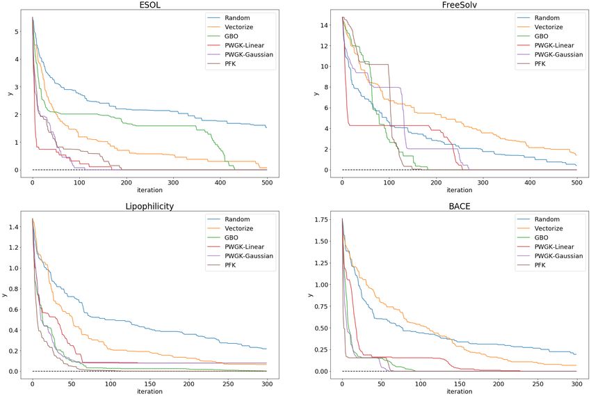
24th European Conference on Artificial Intelligence - ECAI 2020
                                                            Santiago de Compostela, Spain

2     BACKGROUND                                                                Bayesian optimization, the point that maximizes the acquisition func-
                                                                                tion is selected as the next evaluation point:
In this section, we briefly review the traditional Bayesian optimiza-
tion algorithm based on Gaussian process and the topological data                                     xt+1 = argmax acq(x).
analysis based on persistent homology.                                                                            x∈Rd

                                                                                There are many acquisition functions including probability of im-
2.1    Bayesian optimization                                                    provement (PI) [13], expected improvement (EI) [16], and lower con-
                                                                                fidence bound (LCB) [22]. The balance between exploitation and ex-
Bayesian optimization (BO) is an effective optimization method for
                                                                                ploration is important for acquisition functions. Exploitation involves
expensive-to-evaluate objective functions [1]. Let us denote the in-
                                                                                evaluation of points in the surroundings of the point observed with
put vector x ∈ Rd and a black box function f : Rd → R. Bayesian
                                                                                the best objective function value, while exploration involves evalua-
optimization tries to find the optimal data point of the following op-
                                                                                tion of points with high uncertainty. EI, which we use in the exper-
timization problem:
                                                                                iments, is the expected value of the difference between the best ob-
                          x∗ = argmin f (x).                                    servation value ybest obtained up to a certain step and the predicted
                                   x∈Rd                                         objective function value f (x).

Since Bayesian optimization does not need derivatives of the ob-                       acqEI (x) = E[max{0, f (x) − ybest }]
jective function for finding the optimal data point, it is particularly                            (
effective when optimizing black-box objective functions. Bayesian                                    σ(x)(ZΦ(Z) + φ(Z)) σ(x) 6= 0
                                                                                                 =                                    ,
optimization is an iterative method, and each step consists of two                                   0                       σ(x) = 0
steps: (i) calculation of a predictive distribution of an objective func-
tion value by a Gaussian process and (ii) selection of the next search          where Z = µ(x)−y  σ(x)
                                                                                                      best
                                                                                                           , and Φ and φ are the cumulative density
point based on an acquisition function.                                         function and probability density function of a standard normal distri-
                                                                                bution, respectively.
Gaussian process: Gaussian process is a generalization of Gaussian
probability distribution [20]. More specifically, Gaussian process de-
scribes the functions of random variables, while Gaussian probabil-             2.2    TDA based on persistent homology
ity distribution describes random scalars or vectors. In Bayesian op-           In TDA, we focus on the shapes of a complex data from the view-
timization, the objective function f : Rd → R is modeled by a                   point of topology. Here, we give an intuitive explanation of one of
Gaussian process, which enables easy calculation of predictive dis-             the TDA methods, namely persistent homology [3, 6]. We analyze
tributions. Now, let { (x1 , y1 ), · · · , (xt , yt ) } be pairs of the input   a point cloud { x1 , · · · , xN } on a metric space (M, c). In case of
and the corresponding output of the objective function observed up              analysis of a compound, the point cloud may be the set of 3D coor-
to a certain step, where xi ∈ Rd , yi ∈ R for i = 1, · · · , t. We as-          dinates of atoms forming the compound. In order to analyze this by
sume that the true value f (xi ) is not necessarily observed as yi , but        persistent homology, we consider the union of balls centered on each
an independent additive Gaussian noise i ∼ N (0, σ 2 ) is included:            point with radius r:

                            yi = f (xi ) + i .                                                        N
                                                                                                       [
                                                                                                Sr =         { x ∈ M | c(x, xi ) ≤ r } .
According to the definition of Gaussian process, the joint probability                                 i=1
distribution of f (x1 ), · · · , f (xt ) is
                                                                                Figure 1 shows examples of Sr . We can observe that topological
                                          T
                  (f (x1 ), · · · , f (xt )) ∼ N (0, K),                 (1)    structures like connected components and rings appear and disap-
                                                                                pear while increasing r. In persistent homology, we focus on when
where 0 = (0, · · · , 0)T , ·T denotes the transpose operator, and each         each topological structure appears and how long it persists.
element of K ∈ Rt×t is expressed by Kij = k(xi , xj ) using
the kernel function k(·, ·). Then, the predictive distribution of the
function value f (xt+1 ) at the point xt+1 , which is not included in
the data, can be calculated. Since the joint probability distribution
of f (x1 ), · · · , f (xt ), f (xt+1 ) is also expressed similar to the ex-
pression (i.e., Eq. (1)) and the additive noise is included in the ob-
servations, the predictive distribution of f (xt+1 ) is also a Gaussian
distribution whose mean µ(xt+1 ) and covariance σ 2 (xt+1 ) can be
calculated as follows:

          µ(xt+1 ) = k(K + σ 2 I)−1 y,
         σ 2 (xt+1 ) = k(xt+1 , xt+1 ) − k(K + σ 2 I)−1 kT ,                    Figure 1. Examples of Sr . We can observe that topological structures like
                                                                                 connected components and rings appear and disappear while increasing r.
where k = (k(xt+1 , x1 ), · · · , k(xt+1 , xt )), y = (y1 , · · · , yt )T .
See [20] for the detailed derivation.
                                                                                   The topological features extracted by persistent homology can be
Acquisition function: The acquisition function acq(x) expresses                 expressed as a point cloud on R2 called a persistence diagram (PD).
the degree to which we should evaluate the input point x based on               A point (b, d) on a PD shows the corresponding topological struc-
the predictive distribution calculated utilizing a Gaussian process. In         ture that appears at radius b and disappears at radius d. b and d are
24th European Conference on Artificial Intelligence - ECAI 2020
                                                              Santiago de Compostela, Spain

called birth and death of the structure, respectively, and d−b is called          multiple topological features extracted by persistent homology by
persistence of the structure. Since b < d, all the points on a PD are             constructing a kernel using kernels calculated from each type of PD.
distributed above the diagonal. We can consider multiple PDs for the                 In this section, we first formulate the topological Bayesian opti-
same point cloud depending on the structure of interest. It is called             mization problem using persistence diagrams. Then, we propose the
the 0th PD when we focus on the connected components, the 1st                     kernel based Bayesian optimization algorithms. We first introduce
PD when we focus on the rings and so on. Figure 2 shows the 0th                   kernels for PDs in Section 3.2, and then explain methods for con-
PD and the 1st PD for the point cloud of Figure 1. The births of all              structing a kernel from multiple kernels in Section 3.3.
points in the 0th PD are 0 because all connected components already
exist at r = 0 and new one does not appear in the middle of in-                   3.1    Problem formulation
creasing r. Two points corresponding to the small ring and the large
ring in the point cloud can be seen in the 1st PD. The small ring                 Let us denote the dataset of PDs by D = { Di }i∈I , where I is the
corresponds to the point closer to the diagonal because it has smaller            set of oracle indices that we cannot observe in the beginning. In addi-
persistence than the large one. A point with small persistence is likely          tion, we assume that evaluating a PD Di is expensive. Since TDA is
to be caused by noise. Thus, the points distributed near the diagonal             highly used in material science, this assumption is rather reasonable.
may represent noisy structures, while the points distributed far from             In this paper, we consider searching for the point that minimizes the
the diagonal may represent more important structures.                             objective function from the dataset D:
                                                                                                         D∗ = argmin f (D),                          (2)
                                                                                                                    D∈D

                                                                                  where f : D → R is a black box function. This problem can be
                                                                                  solved easily if we can examine all possible cases. However, since
                                                                                  the objective function is expensive to evaluate, we need to find the
                                                                                  optimal data point with a small number of evaluations. We also as-
                                                                                  sume that the objective function value can be observed only in a state
                                                                                  of including the independent additive Gaussian noise i ∼ N (0, σ 2 ).
                                                                                  Note that we search for the optimal PD from the given dataset D
                                                                                  which we generate from the given dataset of structured data. Since
                                                                                  we know all possible PDs and the corresponding structured data, we
                                                                                  do not consider about the inverse problem. That is, we need not to
                                                                                  reconstruct a structured data from a PD. The final goal of this paper
                                                                                  is to develop a Bayesian optimization algorithm to solve Eq. (2).
Figure 2. 0th and 1st PDs for the point cloud of Figure 1. The births of all
points in the 0th PD are 0 because all connected components already exist at
 r = 0. Two points corresponding to the small ring and the large ring are in      3.2    Kernels for persistence diagrams
 the 1st PD. The smaller ring corresponds to the point closer to the diagonal
 because it has smaller persistence than the large one. These points are often    There have been several kernels for persistence diagrams. We use the
treated as noisy structures since small persistences are likely to be caused by   persistence weighted Gaussian kernel proposed by Kusano et al. and
                noise in data (i.e. the point cloud of Figure 1).                 the persistence Fisher kernel proposed by Le and Yamada. In this
                                                                                  section, we introduce these kernels.

   In this section, we gave the explanation of persistent homology                Persistence weighted Gaussian kernel [12]: Persistence weighted
based on a fattened ball model which is applicable only to point                  Gaussian kernel (PWGK) considers a PD as a weighted measure. It
cloud data, since it is easy to intuitively understand persistent ho-             first vectorizes the measure on an RKHS by kernel mean embedding,
mology while associating it with the concept of holes. However, we                and then uses conventional vectorial kernels such as linear kernel
can also apply persistent homology to images and graphs and extract               and Gaussian kernel on the RKHS. More specifically, it considers
persistence diagrams from them [10]. There is more general explana-               the following weighted measure for a persistent diagram D:
tion based on sublevel sets which is applicable to these various data                                             X
(e.g. images and graphs) [6].                                                                              µD =       w(x)δx ,                   (3)
                                                                                                                    x∈D

                                                                                  where δx is a Dirac measure, which takes 1 for x and 0 for other
3    PROPOSED METHOD                                                              points. Additionally, Dirac measures are weighted by the weight
In order to handle structured data by Bayesian optimization, it is nec-           function w(x) : R2 → R based on the idea that the points close
essary to design a similarity that captures the topological features of           to the diagonal in the PD may represent noisy features, while the
a structure. Although TDA has attracted considerable attention as                 points far from the diagonal
                                                                                                         P     may represent relatively important fea-
techniques that can extract such features from complex data, there                tures. Let E(µD ) =      x∈D w(x)k(·, x) be the vector representa-
has been no Bayesian optimization method utilizing TDA to design                  tion of µD embedded by kernel mean embedding into the RKHS H
                                                                                                                                   2
the similarity. Therefore, in this paper, we propose Bayesian opti-               using Gaussian kernel k(x, y) = exp − kx−yk 2ν 2
                                                                                                                                     . Then, the linear
mization utilizing features extracted by persistent homology.                     kernel of persistence diagrams Di , Dj on the RKHS is
   Moreover, most studies on the applications of persistent homology
to machine learning, especially studies on kernels for PDs, consider                 kL (Di , Dj ) = hE(µDi ), E(µDj )iH
one type of PD extracted from one data to calculate the kernel. How-                                  X X
                                                                                                                               kx − yk2

ever, it is possible to extract multiple types of PD from one data by                              =            w(x)w(y) exp −            ,
                                                                                                                                 2ν 2
using persistent homology. We further propose methods to handle                                      x∈D y∈D
                                                                                                          i     j
24th European Conference on Artificial Intelligence - ECAI 2020
                                                        Santiago de Compostela, Spain

where ν > 0 is the kernel bandwidth. In addition, the Gaussian ker-        Kernel target alignment: A method of maximizing a value called
nel on the RKHS is                                                         alignment was proposed to learn α [4]. It first considers the centered
                                                        !                  Gram matrix Kc for the Gram matrix K:
                               kE(µDi ) − E(µDj )k2H
        kG (Di , Dj ) = exp −                             .                         (Kc )ij = Kij − Ei [Kij ] − Ej [Kij ] + Ei,j [Kij ].
                                         2τ 2
                                                                           Then, the alignment of two Gram matrices K, K 0 is as follows:
Here, τ > 0 and kE(µDi ) −           E(µDj )k2H   = kL (Di , Di ) +                                             hKc , Kc0 iF
kL (Dj , Dj )−2kL (Di , Dj ). We will refer to them as PWGK-Linear                             κ(K, K 0 ) =                   ,
                                                                                                               kKc kF kKc0 kF
and PWGK-Gaussian, respectively.
   Note that PWGK can be efficiently approximated using ran-               where h·, ·iF is the Frobenius inner product and k · kF is the Frobe-
dom Fourier features [18]. This method uses the random variables           nius norm. In the alignment-based     method [4], we maximize the
                                                                           alignment of K = i αi Ki and Y = yy T . Maximization of the
                                                                                                P
z1 , · · · , zM from the normal distribution N ((0, 0), ν −2 I) to ap-
proximate kL (Di , Dj ) by                                                 alignment results in the following quadratic programming problem:
                                                                                                    min v T M v − 2v T a,
                                    M                                                               v≥0
                                 1 X m m ∗
                 kL (Di , Dj ) ≈       Bi (Bj ) ,                          where
                                 M m=1
                                √                                              Mij = hKic , Kjc iF , a = (hK1c , Y iF , · · · , hKkc , Y iF )T .
                                                         ∗
        Bim
                 P
where      =      x∈Di w(x) exp  −1zm x and                  denotes the
                                                                           Let v ∗ be the solution of this problem. Then, the coefficients are
complex conjugate.
                                                                           calculated by α = v ∗ /kv ∗ k. Since y is updated at each step in
Persistence Fisher kernel [14]: Persistence Fisher kernel (PFK)            Bayesian optimization, learning is performed when a new observa-
considers a PD as the sum of normal distributions and measures the         tion is obtained at each step.
similarity between the distributions by using the Fisher information
                                                                           Marginal likelihood maximization: In Bayesian optimization, the
metric. Let Di∆ and Dj∆ be the point sets obtained by projecting
                                                                           objective function is modeled by a Gaussian process. Therefore,
persistence diagrams Di and Dj on the diagonal, respectively. PFK
                                                                           given the outputs of the function obtained up to a certain step y =
compares Di0 = Di ∪ Dj∆ and Dj0 = Dj ∪ Di∆ instead of compar-
                                                                           (y1 , · · · , yt )T , the log marginal likelihood of y can be calculated by:
ing Di and Dj . It makes the sizes of each point cloud equal, which
makes it easy to apply various similarities. Then, it considers the fol-                        1                    1
                                                                               log p(y|α) ∝ − log |K + σ 2 I| − y T (K + σ 2 I)−1 y.
lowing summation of normal distributions for Di0 :                                              2                    2
                                                                           We consider the use of marginal likelihood maximization to learn α.
                              1 X                                          This can be performed by a gradient-based optimization method [2].
                     ρDi0 =        N (µ, νI),
                              Z  0                                         As in the case of kernel target alignment, we learn the coefficients
                                µ∈Di

                         RP                                                when a new observation is obtained.
where ν > 0 and Z =           µ∈Di0 N (x; µ, νI)dx is the normaliza-
tion constant. The Fisher information metric of the probability distri-    4    RELATED WORK
butions ρDi0 and ρDj0 is as follows:
                                                                           Bayesian optimization is widely used for optimizing expensive-to-
                                 Z q                                     evaluate, black-box, and noisy objective functions [1]. For example,
       dF IM (Di , Dj ) = arccos     ρDi0 (x)ρDj0 (x)dx .                  it is used for automated tuning of hyperparameters in machine learn-
                                                                           ing models [21], path planning of mobile robots [15] and finding
The integral appearing in Z and dF IM is calculated using the func-        the optimal set of sensors [8]. Although most studies on Bayesian
tion value at Θ = Di ∪ Dj∆ ∪ Dj ∪ Di∆ . Finally, PFK is expressed          optimization including these studies consider vectorial data as in-
as follows using the Fisher information metric:                            put, there are few studies that consider structured data such as point
                                                                           clouds and graphs.
              kP F (Di , Dj ) = exp(−tdF IM (Di , Dj )),                       The graph Bayesian optimization (GBO) was proposed as a frame-
                                                                           work of Bayesian optimization for graph data in particular for tree
where t > 0 is the tuning parameter.                                       structured data [19]. Then, it was recently extended to an arbitrary
  PFK can also be efficiently computed by approximating ρ by fast          graph structure [5]. GBO proposed by [5] uses a linear combina-
Gauss transform [17]. We use their implementation5 .                       tion of two kernels. One is a conventional vectorial kernel such as
                                                                           linear kernel and Gaussian kernel for the explicit feature vector in-
3.3    Multiple kernel learning                                            cluding the number of nodes, average degree centrality, and average
                                                                           betweenness centrality. The other one is a graph kernel, which may
In order to handle multiple topological features, we construct an ad-      capture the implicit topological features that cannot be expressed by
ditive kernel calculated from each feature. In particular, we consider     explicit features. The coefficients of the linear combination is learned
a linear combination of k Gram matrices K1 , · · · , Kk :                  through the Bayesian optimization process. After that, we can ana-
                                                                           lyze which features expressed by the vectorial kernel or the graph
                     K = α1 K1 + · · · + αk Kk ,                     (4)
                                                                           kernel were effective as a result. Specifically, they used the auto-
where αi ≥ 0 for all i. This construction makes it possible to main-       matic relevance determination squared exponential (SEARD) kernel
tain the positive definiteness of each kernel. We consider two meth-       as a vectorial kernel and the deep graph kernel based on subgraphs
ods to learn the coefficient parameter α = (α1 , · · · , αk )T .           [25] as a graph kernel. However, to the best of our knowledge, there
                                                                           is no Bayesian optimization framework that explicitly uses topologi-
5   http://users.umiacs.umd.edu/˜morariu/figtree/                          cal information.
24th European Conference on Artificial Intelligence - ECAI 2020
Santiago de Compostela, Spain
5 EXPERIMENTS 1. Randomly choose (x0 , y0 ) ∈ [0, 1] × [0, 1].
2. Iterate the following procedure M times.
In this section, we evaluate our proposed algorithms using synthetic
and four real datasets about properties of molecules. (a) Randomly choose r ∈ [2.0, 4.3].
(b) Generate a point cloud { (x1 , y1 ), · · · , (xN , yN ) } according
5.1 Setup to the following recurrence relations:
For the proposed method, we use marginal likelihood maximization xn+1 = xn + ryn (1 − yn ) mod 1,
like as described in Section 3.3 for estimating the noise parameter σ yn+1 = yn + rxn+1 (1 − xn+1 ) mod 1.
in Bayesian optimization.
We set the hyperparameters of PWGK and PFK according to the
The point clouds generated for r = 2.0 and r = 4.3 are shown
original papers [12] and [14], respectively. Let { D1 , · · · , Dn } be
in Figure 3. We use the value of r, which was used to generate a
the PDs for each point cloud in a dataset. In PWGK, we use the
point cloud, as the label of the point cloud. In this experiment, we
weight function:
find the PD of the point cloud with minimum r by using Bayesian
w(x) = arctan(Cpers(x)p ), optimization algorithms.
where pers(x) = d − b for x = (b, d). Therefore, the hyperparam-
eters of PWGK-Linear are C and p in the weight function and the
kernel bandwidth ν. PWGK-Gaussian includes τ in addition. We fix
the hyperparameters with the following values:
• C = median { pers(Di ) | i = 1, · · · , n },
• p = 5,
• { ν(Di ) | i = 1, · · · , n },
ν = median
• τ = median E(µDi ) − E(µDj ) H i < j ,
where
pers(Di ) = median { pers(xj ) | xj ∈ Di } ,
ν(Di ) = median { ||xj − xk || | xj , xk ∈ Di , j < k } .
The hyperparameters of PFK are ν and t. We search these parameters Figure 3. Illustrative examples of synthesized data.
from ν ∈ { 10−3 , 10, 103 } and 1/t ∈ { q1 , q2 , q5 , q10 , q20 , q50 },
where qs is the s% quantile of { dF IM (Di , Dj ) | i < j }.
We compare our proposed algorithm with the random search base-
line and GBO [5]. For GBO, since the synthetic data is given as a Figure 4 shows averages of the minimum observation obtained at
point cloud, we first compute a 5 nearest-neighbor graph and then each step for the synthetic dataset over 30 BO runs. As we expected,
feed the graph into GBO. We use the same kernels as used in the orig- the topological Bayesian optimization methods outperformed ran-
inal paper. We extract 5 features from a graph (the number of nodes, dom search baseline and the GBO algorithm.
the number of edges, average degree centrality, average betweenness
centrality, and average clustering coefficient). Each element x is nor-
malized by x̃ = (x − xmin )/(xmax − xmin ). The window size
and embedding dimension for the deep graph kernel are chosen from
{ 2, 5, 10, 25, 50 }. The kernel bandwidths in the SEARD kernel and
the coefficients of the linear combination are estimated by marginal
likelihood maximization. We also compared with the method only
using the SEARD kernel.
In Bayesian optimization, we randomly choose 10 data points to
calculate the predictive distribution for the first search point. We use
PWGK-Linear, PWGK-Gaussian and PFK as the kernel for PDs and
EI as an acquisition function. We first calculate the 1st PDs for syn-
thetic dataset, and the 0th PDs for real datasets. We calculate these
kernels using approximation methods (random Fourier features for
PWGK and fast Gauss transform for PFK, respectively). We conduct
Bayesian optimization 30 times.
5.2 Synthetic dataset
Figure 4. Comparison between random search baseline, GBO and PD
To generate the synthetic dataset, we used the method proposed in kernels using the synthetic dataset. The black dotted line shows the objective
[9]. This method generates a point cloud on [0, 1] × [0, 1]. We gen- function value of the target data that we want to search for.
erate M = 1000 point clouds consisting of N = 1000 points as the
dataset. The specific procedure is as follows.24th European Conference on Artificial Intelligence - ECAI 2020
Santiago de Compostela, Spain
Figure 5. Comparison between random search baseline, GBO and PD kernels using four real datasets. The black dotted line shows the objective function
value of the target data that we want to search for.
5.3 Real datasets bining the information of the 0th PD and the 1st PD (i.e., k = 2
in Eq. (4)). We compare the cases of using only the 0th PD, using
We use four real datasets about the properties of relatively small com- only the 1st PD and combining both information using kernel tar-
pounds from MoleculeNet [24]. ESOL is a dataset about the water get alignment (KTA) and marginal likelihood maximization (MLM)
solubility of 1128 compounds. FreeSolv is a dataset about the hydra- as methods for learning the coefficients. When combining the PFKs,
tion free energy of 642 compounds in water. Lipophilicity is a dataset we first conduct experiments similar to those in the previous section
about the octanol/water distribution coefficient of 4200 compounds. using only one type of PD and optimize the hyperparameters in each
BACE is a dataset about the binding results for a set of inhibitors of PFK, and then we learn the coefficients of a linear combination.
human β-secretase 1 of 1513 compounds. The average numbers of The results are summarized in Table 1. We evaluate the perfor-
atoms in each dataset are 25.6, 18.1, 48.5, 64.7, respectively. For our mances according to the area under the convergence curve:
method, we treat a compound as a point cloud using only the 3D co-
ordinates of each atom forming the compound without considering T
X
(t)
any other information about atoms or bonds. We find the PD of the ybest − ybest ,
compound with the minimum property such as water solubility and t=1
hydration free energy by using the Bayesian optimization algorithms. (t)
Figure 5 shows the averages of the minimum observation obtained where T is the number of iteration, ybest is the minimum value ob-
at each step for real datasets. In each case, we can see that the infor- served before the tth iteration and ybest is the minimum function
mation of PDs contributes to efficient search for the optimal struc- value. That is, we calculate the area between the convergence curve
ture. Our method shows comparable or better results than existing and the black dotted line in Figure 4 and 5. The values in the table
methods. Our method outperforms especially in the case of the ESOL are scaled so that the case of random search baseline becomes 1.
dataset, which may show that molecular structure reflects some fac- The performances of PWGK-Linear and PWGK-Gaussian are im-
tors associated with water solubility. proved by combining the information of both PDs in many datasets.
However, PFK get worse in many cases. Perhaps, this is because
we perform optimization of kernel parameters and coefficients sep-
5.4 Effectiveness of multiple kernel learning
arately. In addition, when we apply PWGK-Linear to the ESOL
We compare Bayesian optimization using only one type of PD and dataset as example, the performance is better when combining by
that using combined multiple types of PD. Here, we consider com- marginal likelihood maximization than when using only the 1st PD.24th European Conference on Artificial Intelligence - ECAI 2020
Santiago de Compostela, Spain
If there is no prior knowledge about which type of PD is effective, In the experiments, we treated a compound as a point cloud. For
this shows that it may be better to combine both PDs than to choose future work, we consider to extend our method to utilize information
one type of PD for intuition. about atoms and bonds as well. For example, we can treat a com-
For example, when analyzing the water solubility of compounds, pound as a graph and directly apply persistent homology using graph
the situation we want to search the compound with some specific wa- filtration. However, we need to appropriately define a function on
ter solubility not only one with the minimum water solubility may be nodes or bonds to use graph filtration, which will be main challenge.
considered. Thus, we conduct another experiment of finding the max-
imizer of an objective function as another simple target compound.
The results are summarized in Table 2. As in the case of finding the
ACKNOWLEDGEMENTS
minimizer, it is shown that PWGK-Linear and PWGK-Gaussian tend H.K. was supported by JSPS KAKENHI 15H01704. M.Y. was sup-
to be improved by multiple kernel learning while PFK often not. ported by the JST PRESTO program JPMJPR165A and partly sup-
ported by MEXT KAKENHI 16H06299 and the RIKEN engineering
Table 1. Comparison between cases of using only one type of PD and of network funding.
using multiple kernel learning methods to find the minimizer of a function.
Synthetic ESOL Free Lipo BACE REFERENCES
Random 1.000 1.000 1.000 1.000 1.000
[1] Eric Brochu, Vlad M. Cora, and Nando de Freitas, ‘A tutorial on
Vectorize 0.747 0.299 1.668 0.371 0.636
bayesian optimization of expensive cost functions, with application to
GBO 0.252 0.479 0.646 0.088 0.092
active user modeling and hierarchical reinforcement learning’, arXiv
PWGK 0th 0.161 0.056 0.663 0.279 0.184 preprint arXiv:1012.2599, (2010).
-Linear 1st 0.153 0.377 1.409 0.261 0.954 [2] Richard H. Byrd, Peihuang Lu, Jorge Nocedal, and Ciyou Zhu, ‘A
KTA 0.166 0.301 1.061 0.336 0.211 limited memory algorithm for bound constrained optimization’, SIAM
MLM 0.090 0.172 0.456 0.263 0.237 Journal on Scientific Computing, 16(5), 1190–1208, (1995).
PWGK 0th 0.151 0.081 0.895 0.162 0.070 [3] Gunnar Carlsson, ‘Topology and data’, Bulletin of The American Math-
-Gaussian 1st 0.158 0.464 1.235 0.179 0.132 ematical Society, 46, 255–308, (2009).
KTA 0.167 0.246 0.878 0.150 0.067 [4] Corinna Cortes, Mehryar Mohri, and Afshin Rostamizadeh, ‘Algo-
MLM 0.338 0.054 0.544 0.264 0.113 rithms for learning kernels based on centered alignment’, Journal of
PFK 0th 0.117 0.115 0.770 0.050 0.056 Machine Learning Research, 13(Mar), 795–828, (2012).
1st 0.073 0.254 0.646 0.123 0.068 [5] Jiaxu Cui and Bo Yang, ‘Graph bayesian optimization: Algo-
KTA 0.092 0.120 0.882 0.062 0.080 rithms, evaluations and applications’, arXiv preprint arXiv:1805.01157,
MLM 0.147 0.090 0.745 0.080 0.252 (2018).
[6] Herbert Edelsbrunner and John L. Harer, Computational Topology: An
Introduction, American Mathematical Society, 2010.
[7] Reza Zanjirani Farahani, Elnaz Miandoabchi, W.Y. Szeto, and Han-
Table 2. Comparison between cases of using only one type of PD and of naneh Rashidi, ‘A review of urban transportation network design prob-
using multiple kernel learning methods to find the maximizer of a function. lems’, European Journal of Operational Research, 229(2), 281–302,
(2013).
Synthetic ESOL Free Lipo BACE [8] Roman Garnett, Michael A Osborne, and Stephen J. Roberts, ‘Bayesian
Random 1.000 1.000 1.000 1.000 1.000 optimization for sensor set selection’, In Proceedings of the 9th
Vectorize 0.774 0.396 1.029 0.688 0.510 ACM/IEEE International Conference on Information Processing in
GBO 0.466 0.195 0.356 0.512 0.026 Sensor Networks, 209–219, (2010).
PWGK 0th 1.153 0.254 1.339 0.606 0.021 [9] Jan-Martin Hertzsch, Rob Sturman, and Stephen Wiggins, ‘Dna mi-
-Linear 1st 0.276 0.284 0.769 0.386 0.112 croarrays: design principles for maximizing ergodic, chaotic mixing’,
KTA 0.273 0.366 1.359 0.378 0.023 Small, 3, 202–218, (2007).
MLM 0.197 0.272 0.988 0.295 0.004 [10] Christoph Hofer, Roland Kwitt, Marc Niethammer, and Andreas Uhl,
PWGK 0th 0.473 0.052 0.835 0.357 0.026 ‘Deep learning with topological signatures’, Advances in Neural Infor-
-Gaussian 1st 0.303 0.199 0.880 0.304 0.047 mation Processing Systems, 1634–1644, (2017).
KTA 0.296 0.056 1.062 0.255 0.034 [11] Kirthevasan Kandasamy, Willie Neiswanger, Jeff Schneider, Barnabas
MLM 0.675 0.117 0.289 0.418 0.080 Poczos, and Eric P Xing, ‘Neural architecture search with bayesian op-
PFK 0th 0.604 0.075 0.747 0.330 0.030 timisation and optimal transport’, Advances in Neural Information Pro-
1st 0.438 0.172 0.574 0.655 0.095 cessing Systems, 2020–2029, (2018).
KTA 0.608 0.142 0.795 0.577 0.058 [12] Genki Kusano, Kenji Fukumizu, and Yasuaki Hiraoka, ‘Kernel method
MLM 1.132 0.186 0.524 0.695 0.037 for persistence diagrams via kernel embedding and weight factor’, Jour-
nal of Machine Learning Research, 18(189), 1–41, (2018).
[13] Harold J. Kushner, ‘A new method of locating the maximum point of
an arbitrary multipeak curve in the presence of noise’, Journal of Basic
Engineering, 86, 97–106, (1964).
6 Conclusion [14] Tam Le and Makoto Yamada, ‘Persistence fisher kernel: A riemannian
manifold kernel for persistence diagrams’, Advances in Neural Infor-
In this paper, we proposed the topological Bayesian optimization, mation Processing Systems, 10027–10038, (2018).
which is a Bayesian optimization method using features extracted by [15] Ruben Martinez-Cantin, Nando de Freitas, Eric Brochu, Jose Castel-
persistent homology. In addition, we proposed a method to combine lanos, and Arnaud Doucet, ‘A bayesian exploration-exploitation ap-
proach for optimal online sensing and planning with a visually guided
the kernels computed from multiple types of PDs by a linear combi- mobile robot’, Autonomous Robots, 27(2), 93–103, (2009).
nation, so that we can use the multiple topological features extracted [16] J Mockus, Vytautas Tiesis, and Antanas Zilinskas, ‘The application of
from one source of data. Through experiments, we confirmed that bayesian methods for seeking the extremum’, Towards Global Opti-
our method can search for the optimal structure from complex struc- mization, 2, 117–129, (1978).
[17] Vlad I. Morariu, Balaji V. Srinivasan, Vikas C. Raykar, Ramani Du-
tured data more efficiently than the random search baseline and the
raiswami, and Larry S. Davis, ‘Automatic online tuning for fast gaus-
state-of-the-art graph Bayesian optimization algorithm by combining sian summation’, Advances in Neural Information Processing Systems,
multiple kernels. 1113–1120, (2009).24th European Conference on Artificial Intelligence - ECAI 2020
Santiago de Compostela, Spain
[18] Ali Rahimi and Ben Recht, ‘Random features for large-scale kernel ma-
chines’, Advances in Neural Information Processing Systems, 1177–
1184, (2008).
[19] Dhanesh Ramachandram, Michal Lisicki, Timothy J Shields, Mo-
hamed R Amer, and Graham W Taylor, ‘Bayesian optimization on
graph-structured search spaces: Optimizing deep multimodal fusion ar-
chitectures’, Neurocomputing, 298, 80–89, (2018).
[20] C. E. Rasmussen and C. K. I. Williams, Gaussian Processes for Ma-
chine Learning, the MIT Press, 2006.
[21] Jasper Snoek, Hugo Larochelle, and Ryan P. Adams, ‘Practical
bayesian optimization of machine learning algorithms’, Advances in
Neural Information Processing Systems, 2951–2959, (2012).
[22] Niranjan Srinivas, Andreas Krause, Sham Kakade, and Matthias
Seeger, ‘Gaussian process optimization in the bandit setting: No re-
gret and experimental design’, In Proceedings of the 27th International
Conference on Machine Learning, 1015–1022, (2010).
[23] Hui Wang, Yanchao Wang, Jian Lv, Quan Li, Lijun Zhang, and Yan-
ming Ma, ‘Calypso structure prediction method and its wide applica-
tion’, Computational Materials Science, 112, 406–415, (2016).
[24] Zhenqin Wu, Bharath Ramsundar, Evan N. Feinberg, Joseph Gomes,
Caleb Geniesse, Aneesh S. Pappu, Karl Leswing, and Vijay Pande,
‘Moleculenet: A benchmark for molecular machine learning’, arXiv
preprint arXiv:1703.00564, (2017).
[25] Pinar Yanardag and S. V. N. Vishwanathan, ‘Deep graph kernels’, In
Proceedings of the 21th ACM SIGKDD International Conference on
Knowledge Discovery and Data Mining, 1365–1374, (2015).You can also read