A BAYESIAN CONJUGATE MODEL FOR THE ESTIMATION OF FRICTION INTENSITY

Stipe Perišić 
Jani Barle
Predrag Đukić
Hinko Wolf

 https://doi.org/10.21278/TOF.451026321
 ISSN 1333-1124
 eISSN 1849-1391

 A BAYESIAN CONJUGATE MODEL FOR THE ESTIMATION OF
 FRICTION INTENSITY

 Summary

 This paper addresses the Coulomb dry friction force as a technical indicator for fast and
efficient condition-based maintenance. To estimate the value of friction force, the Bayesian
analysis is used. Instead of the complex Markov Chain Monte Carlo numerical method, a
closed-form analytical solution is applied. Thus, a simple and efficient procedure for friction
estimation is described. Such a solution in the Bayesian context is known as the conjugate
prior. The procedure presented here is verified numerically and experimentally by directly
comparing the estimated value with the measured one. Two families of conjugate priors, the
gamma-exponential and the normal-gamma, are compared. It is shown that the latter is
suitable for friction estimation. An additional parameter, the precision parameter, was
proposed as a criterion for the acceptance of estimation.

Key words: Bayesian inference, Conjugate priors, Coulomb dry friction, Experimental
 friction estimation

1. Introduction
 From the diagnostic perspective, the parameter estimation is a key aspect in a successful
damage assessment and consequently in failure prediction. Generally, in diagnostics, if some
measurable value is well correlated with the system condition, it can be used as a technical
indicator. When considering the cases involving mechanical contact, the friction force is the
first choice for an indicator. The problem that arises is how to develop fast and efficient data
processing, which can be further included in the condition-based maintenance (CBM) [1–3].
Since mechanical contacts are unwanted occurrences, they should be detected in the early
development stage. Therefore, an additional requirement is the ability to detect small
quantities. A general CBM approach with two phenomenologically different distributions is
presented in Fig. 1. The parameter density distribution, f(r|Ti), is related to the system
condition at a given time instance. It captures the technical indicator uncertainty due to
different sources, for example the sensor noise and ambient condition. As the system
deteriorates over time, the indicator value changes. This is observed by diagnostic detection
points noted as T1, T2 and Tn in Fig. 1. Since the failure is a future event, the failure
distribution, f(Δt|Tn), is a model of the remaining useful life. To predict failure, the threshold

TRANSACTIONS OF FAMENA XLV-1 (2021) 63

S. Perišić, J. Barle, P. Đukić, H. Wolf A Bayesian Conjugate Model for
 the Estimation of Friction Intensity

should be preset. Then, with more detection points, a better prediction is obtained [4]. The
focus of this paper is not on the failure level settings or the CBM prediction phase but on a
technically simple and efficient time-domain procedure for the estimation of friction.

 Fig. 1 A schematic diagram of condition-based maintenance

 For the systems with a stationary operating point, diagnostics can be performed without
detecting its intrinsic values. Subsequently, a simple amplitude analysis, such as RMS, can be
performed [4]. The analysis that will be presented here, applies to the systems with a
dominant first mode, with frequent changes of the operating point. Therefore, short vibrating
intervals without external energy input are expected. Within the conventional identification
approach, an extended interval of free decay periods must be acquired. From the diagnostic
standpoint, this is not feasible and friction estimation should be performed by analysing just a
few periods. Therefore, it is crucial to have an additional criterion to evaluate the estimation
before acceptance.
 For most mechanical systems, the aging process causes a bigger change in the friction
force (r) than in the mass (m) and the stiffness (k), such as oil film loss or lubricant
deterioration. In those cases, direct methods and more complex monitoring can be used [5].
This paper presents the way how to use the friction force as a technical indicator directly
correlated to damage, but indirectly measured from system response. Herein, the second-order
mechanical system with dry friction is analysed. Among friction models [6,7], the Coulomb
model is a model which is commonly used due to its simplicity [8–10]. It can be found as a
damping model in dry and foil gas bearings [11,12], or in cases involving oil film loss
[13,14]. When the Coulomb friction model is applicable, the equation of motion is Eq. (1).
 + + = (1)
 For the free decay case, the analytical solution exists and can be found in [15,16]. It is a
well-known fact that in the presence of dry friction, free-response amplitudes decay linearly,
i.e. the envelope is a straight line with a constant slope [17]. The slope, and therefore the
friction force, can be estimated from at least two consecutive amplitudes. Due to the noise and
uncertainty, the friction estimation must be in the form of a distribution. In this paper, any
discrepancy difference between the model and the acquired signal, regardless of the cause,
will be considered as noise. More details about this can be found in section 4. In the real
conditions, the Bayesian analysis provides the parameter estimation from the first detection
instance [18]. It combines the prior distribution with some evidence to obtain a posterior
distribution [19]. Since the system changes due to degradation, as shown in Fig. 1, the
succeeding runs cannot be taken as a sample from the same population. The parameters are
then monitored through an update process. This means that the posterior distribution from the
previous detection point becomes the prior distribution to the current detection point. To

64 TRANSACTIONS OF FAMENA XLV-1 (2021)

A Bayesian Conjugate Model for S. Perišić, J. Barle, P. Đukić, H. Wolf
the Estimation of Friction Intensity

estimate the parameter value, as many detection instances as possible should be considered as
successful. The Bayesian analysis presented here will provide a means for accepting and
estimating the parameter, even when a small data set occurs. Due to multidimensionality, the
Bayesian analysis usually implies the Markov Chain Monte Carlo (MCMC) numerical
integration. This is an efficient but complex method that involves an additional sampling
algorithm [20,21]. A different parameter estimation approach can be used instead by applying
an analytical solution, i.e. a conjugate prior. From an engineering standpoint, these analytical
solutions should be considered.
 Therefore, a fast and efficient friction estimation procedure using a conjugate prior is
proposed in this paper. In brief, the conjugate prior is the case when the prior and the posterior
distribution have the same algebraic form [22]. There are a few conjugate priors and they are
mainly applicable to one-dimensional problems. Here, to estimate the Coulomb friction force,
two conjugate models are compared, namely a simple one-dimensional gamma-exponential
model [23] and a two-dimensional normal-gamma model [24]. Also, uncertainty is relatively
easily estimated within the same theoretical assumption by calculating the credibility
intervals, often on a very small data set. In the CBM diagnostic phase, due to the small data
set, the credibility intervals are expected to be wide. Therefore, an additional precision
parameter is proposed as a criterion for the acceptance of signal and estimation.
 To demonstrate the proposed procedure in a real, but controlled environment, a single
degree of freedom testbed is developed. The main feature of the testbed is precise vertical
motion with minimal damping, which is achieved through an air bearing [25]. The friction
force is induced externally and estimated on the acceleration free decay signal. The estimated
friction force distribution is compared to the friction force directly measured by a force
sensor.

2. The Bayesian conjugate prior for friction estimation
 According to Eq. (1), the amplitudes in the free response decays linearly. The friction
force, r, and the envelope free decay slope, y, are related by Eq. (2), where ω0 is the natural
frequency, while k is the stiffness [17,26].
 2 
 = (2)
 
 A series of ideal measurements will yield the same slope for any consecutive two peaks.
In the real-life signal, this is not the case and different values are estimated even for different
amplitudes of the same run. Since uncertainty is present, a Bayesian analysis is a reasonable
choice for parameter density [20], i.e. friction force estimation, at any detection point, as
shown in Fig. 1. The parameter density consists of the aleatory and the epistemic uncertainty
[27,28]. The former is caused by the loss of signal information, such as the noise which or an
improper sampling rate. The epistemic uncertainty is due to the selection of a model. The
Bayesian mathematical expression is shown by Eq. (3).
 | 
 | = (3)
 ∫ | 
 This expression is a combination of the prior distribution, , of the parameter
vector, , and the likelihood function, | , which yield the posterior distribution,
 | . The prior distribution represents the belief about the parameter value before the data
has been acquired. The choice of the prior distribution must be supported by an expert opinion
or previous knowledge to ensure the convergence. A too wide or narrow prior distribution
means very slow convergence [23]. The likelihood function is a statistical model that defines

TRANSACTIONS OF FAMENA XLV-1 (2021) 65

S. Perišić, J. Barle, P. Đukić, H. Wolf A Bayesian Conjugate Model for
 the Estimation of Friction Intensity

the difference between the acquired data and the proposed model [29]. The prior distribution
and the likelihood function form the numerator, which is scaled by a denominator, often
referred to as the normalization constant.
 The Bayesian updating process is as follows. When the first data set (free decay), which
corresponds to the detection point T1 in Fig. 1, is acquired and adopted, the likelihood
function and the prior distribution form the first posterior distribution. After the second data
set, the detection point T2, the posterior distribution from T1, should be taken as the prior
distribution for T2, and so on. Thus, in the updating process, different data sets are used to
establish the density f(r|Ti). In the updating circle from the prior to the posterior distribution,
there are some combinations which yield a fully analytical, closed-form solution for Eq. (3).
This solution is referred to as a conjugate prior. The conjugate prior implies the prior and the
posterior distribution in the same functional form leading to a highly efficient parameter
estimation. The list of conjugate priors is limited, and the selected pair must be well-argued
and justified by an example. In this paper, two families of conjugate priors will be addressed.
 In every real-life system response noise is present and it is typically modelled according
to a normal distribution. Therefore, it would be reasonable to assume the same random model
for the slope derived from every successive amplitude. Based on this assumption, the
estimation of friction can be performed via a conjugate prior. As stated previously, there is a
limited number of conjugate priors, but when the model is a normal distribution, the normal-
gamma distribution presented here in Eq. (4) is a conjugate prior.
 
 , | , , , = (4)
 √2 
 This is a bivariate distribution, and r and s in Eq. (4) are the variables, i.e. the friction
force and the precision parameter, respectively, which are the system parameters of interest.
The precision parameter is just the inverse of variance, so this family of conjugate priors
provides an estimation of the average deviation between the proposed model and the acquired
data. However, to obtain only the friction force distribution, as shown in Fig. 1,
marginalization has to be performed. Since the complex friction process is approximated by
the Coulomb model, the friction force parameter variance can be large. In that case, the
precision parameter is chosen as a control parameter to additionally support the estimation.
The notations μH, λH, βH, αH represent the distribution parameters. The distribution parameter
μH is related to the mean value of r, with the standard deviation related to λH. The parameters
αH and βH refer to the precision parameter s. The mean value and the standard deviation are
set according to the principles of gamma distribution. This means that the mean value is the
ratio between αH and βH with a standard deviation of αH/β2H. Equation (4) represents the prior
and the posterior distribution. The only difference between them is in the parameter values.
Parameters in Eqs. (5- 8) marked with the subindex 0 are related to the prior distribution
which reflects our initial about the system parameters r and s. Regardless of the acquired data,
these parameters are set according to the initial information (expert opinion). The parameters
marked with H are the so-called hyper-parameters related to the posterior distribution. They
are a result of derivation from Eq. (3) and can be calculated according to Eqs. (5- 8)
 ̅
 μ = (5)

 λ = + (6)

 α = + (7)

66 TRANSACTIONS OF FAMENA XLV-1 (2021)

A Bayesian Conjugate Model for S. Perišić, J. Barle, P. Đukić, H. Wolf
the Estimation of Friction Intensity

 ̅
 β =β + ∑ − ̅ + (8)

 In Eqs. (5- 8), ̅ is the mean of samples, while n is the number of considered data.
Additional information on this conjugate prior model can be found in [24] and similar
information on the chi-square conjugate prior model in [30].
 The objective of Bayesian analysis is to use the simplest possible model. Therefore, the
previous model will be compared to the frequently used one-dimensional gamma-exponential
model [23], represented by Eq. (9).
 
 | , = (9)
 
 Notations and к represent hyper-parameters, which can be calculated by Eqs. (10-
11). The subindex 0 denotes prior parameters, while r and n are the friction forces and the
number of considered data, respectively.
 = + (10)

 к =к +∑ (11)
 As it will be shown, this is a rather fast and efficient procedure, and as long as one
parameter is to be estimated, the proposed method applies to any system. Otherwise, the more
complex MCMC method has to be used.

3. Numerical example of friction estimation
 To demonstrate the efficiency of the friction estimation procedure, numerically
simulated data with known parameter values were analysed. By doing so, the epistemic
uncertainty, which is always present when dealing with a real-life problem, is completely
excluded from the analysis. The Coulomb friction force is set to 0.07 N, the mass is 10 kg and
the stiffness is 1000 N/m. The Gaussian noise with a zero mean value and a standard
deviation (σ) of 5e-4 were added to the simulated response. This yields a signal-to-noise ratio
(SNR) of 20 dB.
 The friction force is assumed to be scattered around the true mean according to a normal
distribution. To test the assumption initially, the same data were analysed with the normal
distribution probability paper. It was found that data can be well approximated with a straight-
line, which preliminary proves the model. In this example, the total length of the analysed
signal was 33 seconds, and all of the 51 amplitudes (evidence) were included in the Bayesian
analysis according to Eqs. (5-8). The graphical representation of the simulated signal is
omitted due to brevity.
 The estimated parameters are shown in Fig. 2. The upper panel represents the prior
distribution, while the lower one represents the posterior distribution after all data
(amplitudes) have been considered. It is important to mention again that the noise model
added to the smooth numerical waveform was a normal distribution with a zero mean and a
standard deviation (σ) of 5e-4. Since only peak amplitudes were analysed, the waveform noise
surely differs from the one related to the amplitudes. This is an important fact since, here, the
precision parameter is directly related to the standard deviation. Hence, the true value of this
parameter is unknown. This can be considered as a disadvantage of the procedure.
Nevertheless, the standard deviation can be roughly estimated via the root mean square error
(RMSE), and its value is 4.3e-4. This provides a reference value by which the Bayesian
analysis should converge.

TRANSACTIONS OF FAMENA XLV-1 (2021) 67

S. Perišić, J. Barle, P. Đukić, H. Wolf A Bayesian Conjugate Model for
 the Estimation of Friction Intensity

 A minor deviation of 0.8 % exists between the true and the estimated friction force,
which is 0.0706 N. The estimated value of precision parameter is 34.3, converting to the
standard deviation, whose value is 8.4e – 4, which is the same order of magnitude as RMSE.
Furthermore, the RMSE estimation falls within the 90% posterior credibility interval. This is
found to be acceptable, particularly considering the prior setup. Generally, the prior
parameters are chosen with sparse knowledge about the true value of each parameter, and the
expected value differs from the true one. Therefore, the prior distribution should cover the
value that it converges to. Due to different limits of axes, which are not immediately visible,
the posterior distribution significantly reduces intervals. The 90% credibility interval now
covers a much smaller area compared to the prior distribution. This is particularly noticeable
in the case of the precision parameter, which suggests a proper model selection and a good
friction parameter estimation.

 Fig. 2 The Coulomb friction force estimated for a simulated response via the normal-gamma conjugate prior

 The impact of aleatory uncertainty is tested on the numerical model, Eq. (1), by
increasing the noise levels i.e. SNR=14.7 dB and SNR=8.6 dB. When compared to the true
friction value, the error is 0.33% and 2.70%, respectively. Even when the noise level
increases, the presented method still remains effective.
 Even though the list of conjugate priors is short, the choice is not simple because not
every conjugate model is suitable for solving the problem. Thus, on the same data set, the
gamma-exponential model, presented by Eq. (9), is analysed. Due to one-dimensionality, this
model does not have a control parameter. The prior and the posterior distribution can be seen
in Fig. 3 on the top and the bottom panel, respectively. The true value is noted with a vertical
red line, while the estimated one with a vertical dashed grey line.

 Fig. 3 The Coulomb friction estimated for a simulated response via the gamma-exponential conjugate prior

68 TRANSACTIONS OF FAMENA XLV-1 (2021)

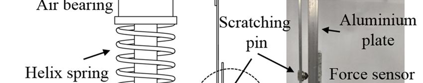
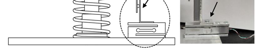
A Bayesian Conjugate Model for S. Perišić, J. Barle, P. Đukić, H. Wolf
the Estimation of Friction Intensity

 Only by observing the posterior distribution width, when the true friction force value is
unknown, the result would be accepted for CBM. This is clearly not the case as it converges
towards an incorrect value. Since the credibility interval is significantly narrowed and does
not include the true value, this conjugate prior is not suitable for the estimation of friction and
cannot be applied in a manner shown in Fig. 1; therefore, it will be left out from the further
analysis.
 The example given in the previous paragraph proves the need to introduce the precision
parameter, which can support the decision on estimation acceptance. This can be additionally
illustrated by the following example in which the total number of periods included in the
Bayesian analysis was varied. Obviously, with more evidence at disposal, the estimation will
be better. As shown in Fig. 4, the precision parameter value is correlated to the friction
estimation, i.e. a higher value of precision parameter indicates a better friction estimation.
Thus, the precision parameter can be a criterion for the diagnostic signal acceptance.

 Fig. 4 Precision parameter and the Coulomb friction in correlation with the data used

 It should be noted that by considering only the absolute value of precision an erroneous
conclusion could be reached. From the diagnostic aspect, it is advisable to have a previously
determined reference value and to draw conclusions based on the comparison. More details
will be presented in the next section. This numerical example undoubtedly shows that it is
possible to obtain an extremely good parameter estimation via the normal-gamma conjugate
prior.

4. Experimental analysis and discussion
 In this section, a testbed shown in Fig. 5 is used to experimentally verify the proposed
procedure. Precise, vertical one-dimensional motion is achieved through an air bearing [25].
Since this configuration produces extremely small damping, an external source, i.e.
mechanical contact, is added. Friction was induced by the metal contact between the
scratching pin on the moving part and the aluminium plate fixed on the stationary part. The
force was managed by increasing or decreasing pressure between those two parts.
The generated force, which was the value of interest, was directly captured by a force sensor.
The system response, which is taken to be a diagnostic signal, was captured by an
accelerometer.
 All signals were acquired via a NI-USB-6251 National Instrument DAQ device, with a
16-bit resolution and a 1000 Hz sampling rate. This is more than satisfactory considering the
natural frequency of the testbed is 2.9 Hz. No additional filtering of the DAQ system was
used. After, the friction force was processed using a Savitzky-Golay filter to refine the
reference value.

TRANSACTIONS OF FAMENA XLV-1 (2021) 69

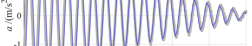
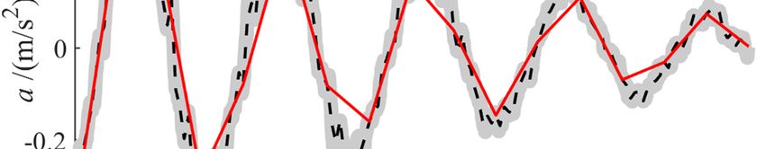
S. Perišić, J. Barle, P. Đukić, H. Wolf A Bayesian Conjugate Model for
 the Estimation of Friction Intensity

 Fig. 5 Experimental setup for the estimation of friction force

 As shown in section 3, the estimation of friction will be obtained by fitting the
envelope, so correct amplitudes ratios are required for the analysis. The linearity and cross-
sensitivity of the sensors were verified in detail, before and after the assembly. For
acceleration, an ADXL322J sensor was used; its operating range is ±2g, the noise in this
configuration is 6.2e-3g. Calibration was performed using a B&K accelerometer, Model 4370,
and a B&K calibrator, Model 4291. The total phase error of the accelerometer signal chain is
0.35 deg. During the operation, an additional displacement sensor was used to check the
signal adopted for the analysis. The sensor is Honeywell SPS-L075-HALS with an operating
range of 0-225 mm and linearity ±0.4%. For friction force, a double beam load cell was used,
with an operating range of ±1 N. The load cell was recalibrated, and its linearity and cross-
sensitivity were tested with a set of laboratory weights; it was also back-to-back tested with a
Tedea Huntley model 1015 load cell in the overload range.
 A typical friction force signal in comparison to the ideal Coulomb model is shown in
Fig. 6. Certain differences can be noticed in the whole segment, which is an aleatory
uncertainty. But at about 3.8, 4, and 4.5 seconds, the difference is more significant, which is
essentially an epistemic uncertainty, i.e. the indication of a more complex model. Since the
signal approximation is satisfying, the Coulomb model is adopted. As the system deteriorates,
the friction force increases, and a more complex model is taken to be unnecessary because the
friction values will be compared relatively. This diagnostic context of the proposed procedure
is an additional reason for adopting this model.

 Fig. 6 A typical friction force signal and the Coulomb model adopted

 The first example presented here is with a higher value of friction force, i.e., the
reference value is 0.2933 N. The acquired acceleration response can be seen in Fig. 7.

70 TRANSACTIONS OF FAMENA XLV-1 (2021)

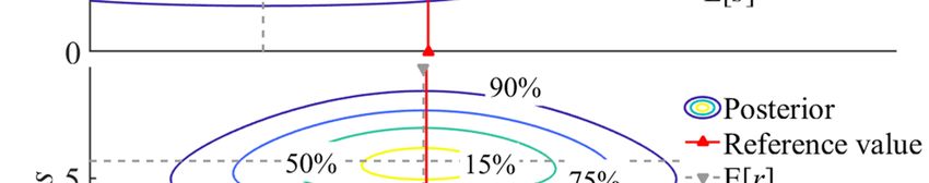
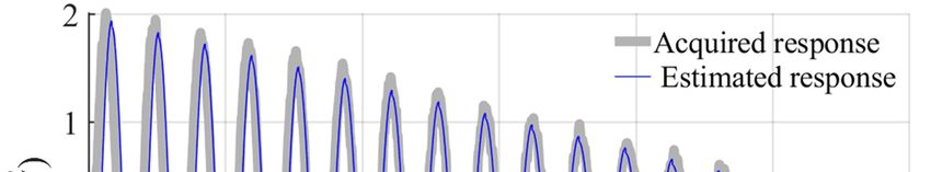
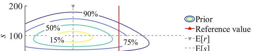
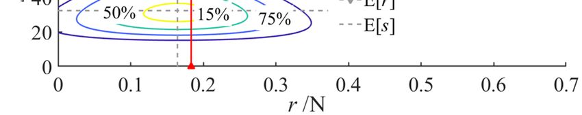
A Bayesian Conjugate Model for S. Perišić, J. Barle, P. Đukić, H. Wolf
the Estimation of Friction Intensity

 Fig. 7 Decaying acceleration amplitudes for the case with a higher value of friction force

 The prior and posterior distributions are shown in Fig. 8. The prior distribution is
relatively wide and is set quite far from the reference value, which emphasizes the uncertainty
in initial parameter values. Despite the prior distribution mean, its width ensures that the
posterior distribution converges near the reference value. The estimate parameters are: a
friction force of 0.2909 N and a precision parameter of 5.7. The estimated values in
comparison to reference values can be seen in Table 2.

 Fig. 8 The Coulomb friction force estimated for the case with a higher value of friction force.

 Besides the point estimation, the distributions also offers additional information. As
noted earlier, the precision parameter is taken to be a control parameter that evaluates the
estimation. As for the precision parameter width, it suggests a proper model selection and a
good friction estimation. However, parameters within the selected model differ. This can be
seen in Fig. 6, where the acquired friction force varies around the mean considerably.
Therefore, the distribution width for the friction force is relatively wide. In these situations, a
different prior selection could provide a more certain estimation if needed. Nevertheless,
regarding the diagnostic context, the estimation is satisfactory. For example, if this estimation
corresponds to the detection point T1, as shown in Fig. 1, then the reference value “slides” to
the right as the degradation progresses. Then, the relatively wide posterior distribution from
the first detection ensures proper updating for the following posterior distribution which
corresponds to the point T2.
 A comparison between the acquired (thick grey) and the estimated (blue) system
response is shown in Fig. 7. It is evident that the amplitude decays linearly, and that the
relative amplitude ratio is appropriate, which means that the estimation is satisfactory. Also,
there is a minor difference between the waveform amplitudes and the periods. This is due to
the fact that only one parameter was analysed. Since other system parameters, mass and

TRANSACTIONS OF FAMENA XLV-1 (2021) 71

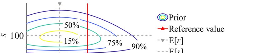
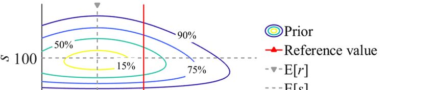
S. Perišić, J. Barle, P. Đukić, H. Wolf A Bayesian Conjugate Model for
 the Estimation of Friction Intensity

stiffness, also affect the resulting waveform, a small deviation can be attributed to them as
well. The characteristic discontinuity due to the friction force is noted on the estimated
waveform. This feature is hardly observed in the acquired response due to the sensor noise.
 The amplitude decay for the second case analysed here is shown in Fig. 9. The thick
grey line represents the acquired response. The reference friction force value is 0.1834 N.

 Fig. 9 Decaying acceleration amplitudes for the case with a lower value of friction force

 The prior and the posterior distribution can be seen in Fig. 10. Same as in the previous
case, the prior distribution is wide and relatively far from the reference value. Here, regardless
of the prior setup, good convergence is also noted, and the posterior distribution width is
significantly reduced. This suggests lower uncertainty in the parameter estimation. The
estimated parameters are the friction force (r=0. 1808 N) and the precision parameter
(s=11.6).

 Fig. 10 The Coulomb friction force estimated for the case with a lower value of friction force

 The difference between the estimated and the recorded value is around 1 %, as noted in
Table 1. However, the precision parameter has a higher value than in the previous case. This
implies a smaller deviation between the presumed model and the acquired data, which in turn
implies higher confidence in the model. This is caused by a lower value of friction force that
affects the total number of periods. If more evidence is used, the confidence is greater. The
acquired system response (thick grey line) and the estimated one (blue line) are shown in Fig.
9. Here, the acceleration discontinuity in the estimated waveform is not emphasized as in the
previous case, due to a lower value of friction force. The same effect is not observed in the
recorded response because of the sensor noise. As already shown, a reasonably good Coulomb
friction force estimation can be obtained by analysing the long, free decay responses. In the
context of CBM, they do not occur frequently. But, before the diagnostic process began, in the
set-up phase, long signals should be used to determine the values of natural frequency ω0 and

72 TRANSACTIONS OF FAMENA XLV-1 (2021)

A Bayesian Conjugate Model for S. Perišić, J. Barle, P. Đukić, H. Wolf
the Estimation of Friction Intensity

stiffness k for Eq. (2). These parameters, as assumed here, are correlated to degradation to a
lesser degree than the friction force r and will not change significantly throughout the process.
 A real diagnostic signal with just a few low-intensity periods and with the initial
condition unknown is simulated in the next case. Therefore, a short segment at the very end of
the signal shown in Fig. 9 is selected. The case to be analysed is shown enlarged in Fig. 15.
The total number of periods is more than five times smaller than the full data set. The prior
distribution is the same as that for the full data set.

 Fig. 11 The acquired signal and a reduced data set

 The estimated parameters are shown in Fig. 12. The posterior distribution width in this
case is significantly greater, which reflects higher uncertainty. Considering the small data set
and the signal-to-noise ratio, it can be concluded that the estimation is reasonably good. The
friction force is 0.1643 N, which gives the difference of 10.3 % relative to the reference value,
and the precision parameter is 32.2.

 Fig. 12 The Coulomb friction force estimated for the reduced data set

 As for the precision parameter, the conclusion would be a more certain estimation
compared to the full data set. However, the precision parameter should not be taken as an
absolute value, but as a relative one with respect to the value derived in similar conditions.
This will be demonstrated later in this section. Here, the high value can be attributed to the
prior set up and the lack of data. Nevertheless, the fact that the precision parameter decreases,
and the interval is much narrower suggests a good estimation. On the other hand, if we
consider only the friction force, the estimation would be rejected because of the large
uncertainty involved. A better estimation, if needed, would be achieved with a more suitable
prior distribution, such as the one in which the data from the previous detection points are
considered. Table 1 shows the estimated friction values in comparison to the reference value
for all three cases.

TRANSACTIONS OF FAMENA XLV-1 (2021) 73

S. Perišić, J. Barle, P. Đukić, H. Wolf A Bayesian Conjugate Model for
 the Estimation of Friction Intensity

Table 1 The friction force estimated for all analysed cases
 Data set1 Data set2 Data set2-reduced
 Estimated value r/N 0.2909 0.1808 0.1643
 Reference value r/N 0.2933 0.1834 0.1834
 Error /% 0.8 1.4 10.4

 It has been shown previously that the proposed procedure can be efficiently applied in
the diagnostic context, i.e. a small number of periods with low intensity. In the following
example we consider the quality of the data, which will be reflected in the precision
parameter. All the cases presented above are with a 1 kHz sampling rate. To simulate 100 Hz
and 10 Hz sampling rates, the down-sampling of the signal in Fig. 11 is performed and shown
in Fig. 13. Thus, by reducing the sampling rate, some pieces of information are lost. In other
words, the aleatory uncertainty increases while the epistemic uncertainty remains the same as
the previous one.

 Fig. 13 A reduced data set with different sampling rates

 The prior distribution for all three sampling rates is shown in the top panel of Fig. 12,
while the posterior distributions are shown in Fig. 14. It is apparent that the discrepancy
between the reference and the estimated friction force increases as the sampling frequency
decreases, which can be seen in Table 2. The first column in Table 2 corresponds to the third
column in Table 1, but here, the precision parameter value is added.
Table 2 The friction force estimated for the reduced data set and different sampling rates
 Sampling rate fs/Hz 1000 100 10
 Reference value r/N 0.1834 0.1834 0.1834
 Estimated value r/N 0.1643 0.1567 0.1465
 Error /% 10.4 14.4 20.1
 Precision parameter s 32.2 32.9 27.5

 The precision parameter s is used to propose the estimation acceptance criteria. In this
experiment, the value of interest is the friction force r; it was directly measured, and the error
could be defined, which is not always possible in real life.
 The signal sampled with a 100 Hz sampling rate still represents the system response
well, and there is no significant information loss. A small discrepancy between the estimated
value of friction and a 1000 Hz sampling rate exists, but the precision parameter is practically
the same. When the sampling frequency is further reduced to 10Hz, information loss occurs,
the error is twice as large and negatively correlated to the precision parameter, as shown in
Table 2.

74 TRANSACTIONS OF FAMENA XLV-1 (2021)

A Bayesian Conjugate Model for S. Perišić, J. Barle, P. Đukić, H. Wolf
the Estimation of Friction Intensity

 Although all three signals are free decay signals, the precision parameters manage to
detect the signal quality and distinguish the better from the worse. Thus, this parameter can be
used as an acceptance criterion when the value of interest cannot be directly measured. For
this particular case, the acceptance criterion could be set to 30. This is something that should
be predefined during the setup phase on a sufficiently long signal.

 Fig. 14 The Coulomb friction force estimated for the reduced data set and different sampling rates

 Since the natural frequency of the experimental setup is 2.9 Hz, relatively high sampling
rates of 1 kHz and 100 Hz provided a reasonably good friction estimation regarding the
diagnostics, which is further supported by the precision parameter. Nevertheless, when the
sampling frequency is significantly reduced, in this case to 10 Hz, the friction estimation is
poor regardless of the fact that the Nyquist frequency criterion is satisfied. Thus, in order for
the proposed analysis to achieve a reasonably good estimation, the sampling rate should be at
least two orders of magnitude higher than the natural frequency.

5. Conclusions
 In this paper, the friction force is chosen as a technical indicator for fast and efficient
condition-based maintenance (CBM) due to the good correlation with degradation. The main
goal was to propose a fast and efficient but technically simple friction estimation procedure
that can be implemented in the condition-based maintenance strategy. In the free decay case,
friction estimation can be performed by calculating the slope on two consecutive amplitudes.
Since real-life situations regarding CBM involve small data sets, noise, and interference, the
same approach could lead to a wrong estimation. Hence, the Bayesian analysis is used to
estimate parameters and the related uncertainty. To avoid complex and time-consuming
numerical methods, a conjugate prior model was used. In the numerical example, it appears
that the gamma-exponential family of conjugate priors is not suitable for friction estimation
while the normal-gamma family of conjugate priors can be efficiently used for that purpose.
The proposed conjugate prior is two dimensional, which means that it estimates the friction
force and the precision parameter. The latter was used as a control parameter, further
supporting the estimated value acceptance when the value of interest cannot be directly
measured. The proposed procedure was evaluated experimentally on the acquired acceleration
free decay responses. An excellent correlation between the estimated and the recorded friction
force was established. Furthermore, the precision parameter suggested a proper parameter
estimation. The same analysis was performed on a reduced data set; a satisfactory friction
estimation was obtained, with a small deviation compared to the full data set. In addition, the
precision parameter suggested a valid estimation.

TRANSACTIONS OF FAMENA XLV-1 (2021) 75

S. Perišić, J. Barle, P. Đukić, H. Wolf A Bayesian Conjugate Model for
 the Estimation of Friction Intensity

 In addition, the proposed analysis was tested regarding the data quality, i.e. the
sampling rate sensitivity. For the analysed testbed, it has been shown that the diagnostic
signal has to be at least two orders of magnitude higher than its natural frequency in order to
obtain a relatively good estimation. The paper proposes an efficient friction force estimation
procedure tested on a laboratory model that can be easily applied in less controlled
environmental conditions.

REFERENCES
[1] J.Z. Sikorska, M. Hodkiewicz, L. Ma, Prognostic modelling options for remaining useful life estimation
 by industry, Mech. Syst. Signal Process. 25 (2011) 1803–1836. doi:10.1016/j.ymssp.2010.11.018.
[2] W. Caesarendra, T. Tjahjowidodo, B. Kosasih, A.K. Tieu, Integrated Condition Monitoring and
 Prognosis Method for Incipient Defect Detection and Remaining Life Prediction of Low Speed Slew
 Bearings, Machines. 5 (2017) 11. doi:10.3390/machines5020011.
[3] E. Quatrini, F. Costantino, G. Di Gravio, R. Patriarca, Condition-Based Maintenance—An Extensive
 Literature Review, Machines. 8 (2020) 31. doi:10.3390/machines8020031.
[4] W. Wang, A model to predict the residual life of rolling element bearings given monitored condition
 information to date, IMA J. Manag. Math. 13 (2002) 3–16. doi:10.1093/imaman/13.1.3.
[5] J. Salgueiro, G. Peršin, J. Vižintin, M. Ivanovič, B. Dolenc, On-line Oil Monitoring and Diagnosis,
 Strojniški Vestn. – J. Mech. Eng. 10 (2013) 604–612. doi:10.5545/sv-jme.2013.973.
[6] E. Pennestrì, V. Rossi, P. Salvini, P.P. Valentini, Review and comparison of dry friction force models,
 Nonlinear Dyn. 83 (2016) 1785–1801. doi:10.1007/s11071-015-2485-3.
[7] F.A.-B. V. Lampaert, J. Swevers, Experimental comparison of different friction model for accurate low-
 velocity cracking, in: Proc. 10th Mediterr. Conf. Control Autom., Lisbon, 2002.
[8] D.A.H. Hanaor, Y. Gan, I. Einav, Static friction at fractal interfaces, Tribol. Int. 93 (2016) 229–238.
 doi:10.1016/j.triboint.2015.09.016.
[9] K. Nakano, Two dimensionless parameters controlling the occurrence of stick-slip motion in a 1-DOF
 system with Coulomb friction, Tribol. Lett. 24 (2006) 91–98. doi:10.1007/s11249-006-9107-7.
[10] M. De Simone, D. Guida, Modal Coupling in Presence of Dry Friction, Machines. 6 (2018) 8.
 doi:10.3390/machines6010008.
[11] R. Hoffmann, R. Liebich, Experimental and numerical analysis of the dynamic behaviour of a foil bearing
 structure affected by metal shims, Tribol. Int. 115 (2017) 378–388. doi:10.1016/j.triboint.2017.04.040.
[12] I. Hutchings, P. Shipway, Applications and case studies, in: Tribology, Elsevier, 2017: pp. 303–352.
 doi:10.1016/B978-0-08-100910-9.00009-X.
[13] G.W. Stachowiak, A.W. Batchelor, Engineering tribology, Second Edi, Butterworth-Heinemann, 2000.
[14] R. Tandler, N. Bohn, U. Gabbert, E. Woschke, Experimental investigations of the internal friction in
 automotive bush chain drive systems, Tribol. Int. 140 (2019) 105871. doi:10.1016/j.triboint.2019.105871.
[15] B.F. Liang, J.W., Feeny, Identifying Coulomb and Viscous Friction from Free-Vibration Decrements,
 Nonlinear Dyn. (1998) 337–347. https://doi.org/10.1023/A:1008213814102.
[16] J.-W. Liang, Identifying Coulomb and viscous damping from free-vibration acceleration decrements, J.
 Sound Vib. 282 (2005) 1208–1220. doi:10.1016/j.jsv.2004.04.034.
[17] W.T. Thomson, Theory of Vibration with Applications, Fourth, Springer US, Boston, MA, 1993.
 doi:10.1007/978-1-4899-6872-2.
[18] D. Kozelj, Z. Kapelan, G. Novak, F. Steinman, Investigating Prior Parameter Distributions in the Inverse
 Modelling of Water Distribution Hydraulic Models, Strojniški Vestn. – J. Mech. Eng. 60 (2014) 725–734.
 doi:10.5545/sv-jme.2014.1741.
[19] T. Ando, Bayesian Model Selection and Statistical Modeling, Taylor and Francis Group, New York,
 2010.
[20] K. Worden, J.J. Hensman, Parameter estimation and model selection for a class of hysteretic systems
 using Bayesian inference, Mech. Syst. Signal Process. 32 (2012) 153–169.
 doi:10.1016/j.ymssp.2012.03.019.
[21] C. Andrieu, N. De Freitas, A. Doucet, I.M. Jordan, An introduction to MCMC for machine learning,
 Mach. Learn. 50 (2003) 5–43. doi:10.1023/A:1020281327116.
[22] B.P. Carlin;, T.A. Louis, Bayesian Methods for Data Analysis Third Edition, 2009.

76 TRANSACTIONS OF FAMENA XLV-1 (2021)

A Bayesian Conjugate Model for S. Perišić, J. Barle, P. Đukić, H. Wolf
the Estimation of Friction Intensity

[23] J. Barle, D. Ban, M. Ladan, Maritime component reliability assessment and maintenance using Bayesian
 framework and generic data, in: Adv. Sh. Des. Pollut. Prev., 2010: pp. 181–188.
[24] M.J. Bernardo, A.F.M. Smith, Bayesian Theory, 3th ed., John Wiley & Sons, 2000.
[25] Q. Gao, W. Chen, L. Lu, D. Huo, K. Cheng, Aerostatic bearings design and analysis with the application
 to precision engineering: State-of-the-art and future perspectives, Tribol. Int. 135 (2019) 1–17.
 doi:10.1016/j.triboint.2019.02.020.
[26] L. Marino, A. Cicirello, Experimental investigation of a single-degree-of-freedom system with Coulomb
 friction, Nonlinear Dyn. 99 (2020) 1781–1799. doi:10.1007/s11071-019-05443-2.
[27] M.E. Paté-Cornell, Uncertainties in risk analysis: Six levels of treatment, Reliab. Eng. Syst. Saf. 54
 (1996) 95–111. doi:10.1016/S0951-8320(96)00067-1.
[28] R. Jordan-Cizelj, I. Vrbanić, Modeling Uncertainties when Estimating Component Reliability, Strojniški
 Vestn. - J. Mech. Eng. 49 (2003) 413–425.
[29] P.L. Green, Bayesian system identification of a nonlinear dynamical system using a novel variant of
 Simulated Annealing, Mech. Syst. Signal Process. 52–53 (2015) 133–146.
 doi:10.1016/j.ymssp.2014.07.010.
[30] S. Brooks, A. Gelman, G.L. Jones, X.-L. Meng, Handbook of Markov Chain Monte Carlo, CRC Press,
 2011. https://doi.org/10.1201/b10905.

Submitted: 14.01.2021 Stipe Perišić
 Jani Barle
Accepted: 22.02.2021 FESB, University of Split, R. Boškovića
 32, 21000 Split, Croatia
 Predrag Đukić
 University department of professional
 studies, University of Split, Kopilica 5,
 21000 Split, Croatia
 Hinko Wolf
 Faculty of Mechanical Engineering and
 Naval Architecture, University of Zagreb,
 Ivana Lučića 5, 10000 Zagreb, Croatia

TRANSACTIONS OF FAMENA XLV-1 (2021) 77