ECONOMIC EVALUATION OF CRYPTOCURRENCY INVESTMENT - MUNICH PERSONAL REPEC ARCHIVE - MUNICH ...

Munich Personal RePEc Archive

Economic Evaluation of Cryptocurrency
Investment

Sakemoto, Ryuta

13 June 2021

Online at https://mpra.ub.uni-muenchen.de/108283/
MPRA Paper No. 108283, posted 15 Jun 2021 00:23 UTC

Economic Evaluation of Cryptocurrency Investment

 Ryuta Sakemotoab

 June 13th, 2021

 Abstract

This study proposes a method to enhance cryptocurrency portfolios constructed by forecast

models. This study forecasts returns on four liquid cryptocurrencies (Bitcoin, Litecoin, Ripple,

and Dash) and determines the weights on the cryptocurrencies based upon a dynamic allocation

framework. We assess the performances of the portfolios using the performance fee measure.

Our results present that the proposed portfolios outperform the benchmark portfolio with the

conventional level of the risk aversion parameter. The economic gain for an investor is

equivalent to 12% per week. The economic gain is sensitive to a change in the risk aversion

parameter, which contrasts with the studies of exchange rates which is due to the high volatility

on the cryptocurrencies. Our predictors are related to the price momentum effects and they

outperform widely used network factors.

Keywords: Cryptocurrency, Bitcoin, Portfolio evaluation, Forecast model, Risk aversion

JEL codes: G10, G11, G17

aGraduate School of Humanities and Social Sciences, Okayama University, Okayama, Japan. 700-8530
Email:ryuta.sakemoto@gmail.com. This work was supported by KAKENHI(20K22092).
b
 Keio Economic Observatory, Keio University, Tokyo, Japan.

 1

1. Introduction

 Cryptocurrencies are regarded as a new asset class and attract significant attention

from both investors and regulators. They present low correlations with other asset classes

such as stocks, bonds, currencies, and commodities (Baur, Dimpfl, and Kuck, 2018;

Kajtazi and Moro, 2019; Klein, Thu, and Walther, 2018; Rognone, Hyde, and Zhang;

2020). Fang, Bouri, Gupta, Roubaud (2019) demonstrate that Bitcoin works as a hedge

for multi-asset investors during an increase in economic policy uncertainty. One of the

reasons that the cryptocurrency market attracts investors is that its high volatility provides

opportunities to create higher returns than those of the traditional assets. For instance,

Corbet, Lucey, Urquhart, and Yarovaya (2019) reported that the Bitcoin price increased

from $616 to $4,800 between October 2016 and October 2017. Biais et al. (2020) propose

an equilibrium model that valuation of a cryptocurrency depends upon transactional

benefits and large volatility is generated without a change in fundamentals.

 In this study, we assess investment strategies for cryptocurrencies in a dynamic

allocation context, because the correlation between cryptocurrencies is low and investors

receive diversification benefits 3 (Ciaian, Rajcaniova, and Kancs, 2018). Platanakis,

Sutcliffe, and Urquhart (2018) show that the equal weight cryptocurrency portfolio

3
 Diversification benefits including cryptocurrencies are explored by Brière, Oosterlinck, and Szafarz
(2015), Dyhrberg (2016) and Guesmi, Saadi, Abid, and Ftiti (2019).

 2

generates a high Sharpe ratio. Platanakis, and Urquhart (2019) consider estimation errors

and improve their previous results. We employ a different approach based upon predicting

a return on each cryptocurrency and determining the weights on the cryptocurrencies.

Adopting forecast models is important for investors since the cryptocurrency markets

have not matured yet and markets may not satisfy the informational efficiency (Urquhart,

2016; Nadarajah and Chu, 2017; Tran and Leirvik, 2020). For example, Chu, Zhang, and

Chan (2019) find that market efficiency of cryptocurrencies varies over time, which is

consistent with the adaptive market hypothesis. Cryptocurrencies have network effects

since users receive benefits from participating in a platform that grows the number of

users (Cong, Li, and Wang, 2020; Liu and Tsyvinsky, 2020; Sockin and Xiong, 2020).

The cryptocurrency markets include bubble periods and are traded by speculators 4

(Cheah and Fry, 2015; Baur, Hong, and Lee, 2018; Corbet, Lucey, and Yarovaya, 2018).

Negative bubbles in cryptocurrency markets are also observed in certain periods (Fry and

Cheah, 2016). These market features imply that considering past price information is

beneficial for investors, as reported by Grosby, Ahmed, and Sapkota (2020), and

4
 Shen, Urquhart, and Wang (2019) and Philippas, Philippas, Tziogkidis, and Rjiba (2020) find that
media attention is a driving force a change in cryptocurrency prices. In contrast, some studies present
that macro fundamentals such as money supply are important in the long-run (Kristoufek, 2015;
Bouoiyour, Selmi, Tiwari, and Olayeni, 2016; Li and Wang, 2017). Schilling and Uhlig (2019)
propose a theoretical model that a monetary policy impacts a cryptocurrency price.

 3

employing forecast models in order to construct a cryptocurrency portfolio enhances the

performance of the portfolio. To this end, we use the portfolio construction approach

proposed by Della Corte, Sarno, and Tsiakas (2009). This allows us to evaluate whether

the forecast models improve the portfolio performance in terms of investor’s perspective.

Moreover, investors adjust total risk on the portfolios with changing the weights on the

cryptocurrencies and the risk-free asset. This is also appealing because the risk on

cryptocurrency portfolios is higher than that on traditional assets5.

 The first contribution of this study is that we evaluate our prediction performance

based upon a dynamic allocation framework. Della Corte et al. (2009) highlight that return

predictability is not directly associated with an economic gain for investors. They propose

a new criterion that is linked to the willingness of investors to pay for switching from a

dynamic allocation portfolio based upon the random walk model to one that is based upon

forecast models. The effectiveness of the criterion is reported in the stock, bond, and

currency markets (Rime, Sarno, and Sojli, 2010; Della Corte, Sarno, and Tsiakas, 2011;

Thornton and Valente, 2012; Ahmed, Liu, and Valente, 2016; Opie and Riddiough, 2020).

 The second contribution of this study is that we explore a relationship between

5
 For instance, risks on the cryptocurrencies in our dataset are more than 200% per annum. See
Table 1.

 4

the risk aversion parameter and the performance measure. The risk aversion parameter

has received attention in the equity market literature and plays an important role to

determine an equity risk premium (e.g. Mehra and Prescott, 1985; Benartzi and Thaler

1995; Campbell and Cochrane, 1999). The previous studies which employ the

performance measure do not explore the effects of the risk aversion parameter since

results are not sensitive to a change in the risk aversion parameter (Della Corte et al.,

2009). Cryptocurrencies, however, both risk and return are much larger than those of the

other assets (e.g. Baur et al. 2018a). This distinct feature of cryptocurrencies may impact

the evaluation framework since less risk averse investors and speculators prefer to invest

in cryptocurrencies (Baur et al. 2018b). Zimmerman (2020) highlights that speculators

play important roles in cryptocurrency valuation. For this reason, the conventional level

of risk aversion may not be reasonable, and hence we consider both the standard risk

averse and less risk averse investors.

 This paper is related to Platanakis et al. (2018) and Platanakis, and Urquhart

(2019), while they do not consider prediction models. Moreover, they do not investigate

a relationship between portfolio performances and investor’s risk aversion. Focusing

upon the investor’s risk aversion is an important difference from the studies of Della Corte

et al. (2009) and Thornton and Valente (2012), since they examine assets which are less

 5

volatile and speculators are not main players in their markets.

 To preview our results, we find that the cryptocurrency portfolios constructed by

the forecast models outperform the benchmark portfolio constructed by the historical

average return model. More importantly, the economic gain for an investor is

large―equivalent to 12% per week. We also note that the investor’s risk aversion plays a

key role in determining the economic gain. This is the contrast result reported by the

previous literature in the exchange rate context, which is due to the high volatility on the

cryptocurrencies.

 The remainder of the paper is organized as follows: Section 2 introduces the data

set we used and the predictive regression model; Section 3 describes statistical and

economic measures in assessing forecast performances; Section 4 reports our main

empirical results; Section 5 demonstrates additional tests; and Section 6 presents our

concludes.

2. Data and Predictive Models

In this section, we introduce cryptocurrency data used in this study. Then, we describe

our predictive model that adopts past price information.

 6

2.1 Data

The data set employed in this study is weekly cryptocurrency market prices against the

U.S. dollar, obtained from coinmarketcap.com.6 We follow Platanakis et al. (2018), and

Platanakis and Urquhart (2019) and employ the four most liquid cryptocurrencies: Bitcoin,

Litecoin, Ripple and Dash. In addition to these four cryptocurrencies, we use Ethereum

for the robustness section.

 The literature in the exchange rates often use monthly data, while it does not

allow us to obtain a long period of monthly data for cryptocurrencies. Following

Platanakis et al. (2018), we focus upon weekly data. We collect every Wednesday prices

since the other assets are also traded then, and thus there is no weekend effect (e.g. Keim

and Stambaugh, 1984). Our data covers the period from 12th July 2015, to 29th July 2020,

and the total observations are 260 weeks. We calculate a return using the weekly close

price. A one-month Treasury bill rate is used as the risk-free rate, which is obtained from

the Kenneth French web-site (e.g. Fama and French, 1993).

2.2 Predictive models

We consider a predictability of return on each cryptocurrency in a time series context.

6 http://www.coinmarketcap.com.

 7

Letting +1 denote a cryptocurrency return at time t+1 and denote a vector of

predictors at time t:

 +1 = + + +1 (1)

where is a constant term, is the vector of the estimated parameters and +1 is an

error term. Following Platanakis et al. (2018), and Platanakis and Urquhart (2019), we

employ weekly data sets. Cheah and Fry (2015) and Corbet et al. (2018) find that bubble

periods in the cryptocurrency markets, which suggests that price momentum is an

important determinant of cryptocurrency prices. Motivated by this finding, we adopt

lagged returns as predictors and we employ from one to four-week lagged returns, since

a one-week lagged return is not sufficient to capture cryptocurrency price fluctuations

(Shen et al., 2019; Grobys et al., 2020) 7. We also employ network factors which are

associated with theoretical models and these are effective at a longer frequency in the

robustness section (Liu and Tsyvinsky, 2020)8.

3. Forecast Evaluation

In this section, we first introduce a statistical evaluation criterion to evaluate each

7
 We do not employ the Bayesian Information criterion since it supports no lagged return.
8
 Bleher and Dimpfl (2019) report that the google search volume does not predict returns on
cryptocurrencies, and therefore we do not focus upon the google search volume.

 8

currency investment forecasting return. Second, we describe the construction of a

portfolio based upon the predictive models and determine weights on the cryptocurrencies.

Third, we explain our approach about transaction costs. Finally, we illustrate forecast

evaluations based upon the portfolios.

3.1. Statistical measure

This section describes the measures used to evaluate the out-of-sample predictive power

 2
for our forecast models. We use the out-of-sample and compare the mean squared

errors (MSE) of the forecast and those of benchmark models (Campbell and Thompson,

2008; Rapach, Strauss, and Zhou, 2013; Risse, 2019). Let ̂ +1 be the forecast

cryptocurrency return based upon the predictive regression model and ̅ +1 the

benchmark return. Following Campbell and Thompson (2008), we adopt the historical

average of realized returns as the benchmark return. Using ̂ +1 and ̅ +1, the out-of-

 2
sample statistic is calculated as follows:

 2
 ∑ −1
 =0 ( +1 − ̂ +1 )
 2
 = [1 − ] (2)
 ∑ −1
 =0 ( +1 − ̅ +1 )
 2

 2
where +1 is the realized return. When > 0, the forecast return ̂ +1 outperforms

the historical average forecast return in terms of MSE. We conduct a statistical test based

upon the adjusted mean squared prediction error statistic (MSPE-adjusted) proposed by

 9

Clark and West (2007). This test statistic extends the Diebold and Mariano (1995), and

West (1996) statistic given its nonstandard distribution when comparing forecasts from

nested models. Following Rapach, Strauss, and Zhou (2010), a p-value for a one-sided

(upper-tail) test is adopted. Our predictive regression models are nested models when we

use the historical average as the benchmark.

3.2. Asset allocation framework

We consider that an investor adopts a dynamic allocation strategy in order to maximize

the conditional expected return subjected to target conditional volatility (Della Corte et

al., 2009, 2011; Rime et al., 2010; Thornton and Valente, 2012; Ahmed et al., 2016). We

consider the following two steps. First, each cryptocurrency one-week-ahead return

forecast is generated by the forecast models described in the previous section. Second,

the optimal weights on the cryptocurrencies are determined on the mean-variance

efficient frontier.

 Let +1 be the × 1 vector of cryptocurrency returns at time + 1 ,

 +1| = [ ] the conditional expectation of and Σ +1| = [( +1 −

 ′
 +1| )( +1 − +1| ) ] the conditional variance-covariance matrix of . An investor

determines the weights on the cryptocurrency portfolios at each time based upon the

 10

following optimization problem:

 max{( , +1| = ′ +1| + (1 − ′ ) , )} (3)
 
 . . ( ∗ )2 = ′ Σ +1| 

where , +1| is the conditional expectation on the portfolio return vector constructed

by the risky cryptocurrency currency portfolio and the risk-free asset , , is a × 1

vector of one, and ∗ is the target conditional volatility on the portfolio returns. The

optimal weights are obtained as the solution to Equation (3) and written as:

 ∗
 = Σ −1
 +1| ( +1| − , ) (4)
 √ 
 ′
where = ( +1| − , ) Σ −1
 +1| ( +1| − , ). Following Ahmed et al. (2016), we

impose a restriction for the optimal weights to avoid extreme values as:− ≤ ≤ 2 .

The gross return of an investor’s optimal portfolio is calculated as follows:

 , +1 = 1 + , +1 = 1 + (1 − ′ ) , + ′ (5)

where 1 − ′ is the weight of the risk-free asset. After obtaining the portfolio return

 , +1 , we assess performances of the predictive models.

3.3 Transaction costs

Our asset allocation framework needs to change weights on cryptocurrencies every week.

We consider transaction costs when we change the weights, and we follow Lintilhac and

 11

Tourin (2017) and Platanakis et al. (2018) and calculate transaction costs. A transaction

cost for cryptocurrency j is calculated as the proportionate cost multiplied by the

change in the weight between t and t-1. Then we aggregate all transaction costs and obtain

the total transaction cost for the portfolio at time t as:

 = ∑ 
 =1 (| , − , −1 |) (6)

where N is the total number of cryptocurrencies.

3.4. Performance measures

We employ two measures to evaluate portfolio performances. The first performance

measure is the Sharpe ratio, which is widely used in the literature (e.g. Campbell and

Thompson, 2008; Barroso and Santa-Clara, 2015). The Sharpe ratio is interpreted as a

risk-adjusted return measure and defined as:

 ̅̅̅̅̅̅̅̅̅
 − 
 
 (7)

where ̅̅̅̅̅̅̅̅̅
 − is the realized average excess return and is standard deviation of the

excess return.

 The second measure is the performance fee measure which is based upon mean-

variance analysis and used in the exchange rate and bond market studies (Della Corte et

al., 2009, 2011; Rime et al., 2010; Thornton and Valente, 2012; Opie and Riddiough,

 ̅ (∙) for an investor with investor’s relative risk
2020). The average realized utility 

 12

aversion (RRA) is constructed by a mean-variance utility function9 (Ahmed et al.,

2016):

 −1
 2 (8)
 ̅ (∙) = ̅ −
 ∑( , +1 − ̅ )
 2 
 =0

 1
where , +1 is the gross return on the investor’s portfolio and ̅ = ∑ −1 . We
 =0 , +1

consider weekly expenses as the maximum performance fee that an investor is willing to

pay to switch from the alternative portfolio to a benchmark portfolio (e.g. Fleming, Kirby,

and Ostdiek, 2001). The performance fee Φ is obtained as the difference between the

 ∗
average utility from the gross portfolio return constructed by a predictive model, , +1

and that from gross benchmark portfolio return, , +1 :

 ̅ ( , +1
 Φ= ∗ ̅ ( , +1
 )− 
 ). (9)

Note that Φ ≤ 0 means that the model has no predictive power.

4. Empirical results

This section shows our data and empirical results. First, we present summary statistics for

our cryptocurrency data. Second, we report out-of-sample return forecasts based upon the

statistical measure. Third, we present out-of-sample portfolio return forecasts based upon

9
 We do not assume a quadratic utility used by Della Corte et al (2009) and Thornton and Valente
(2012), since numerical procedures are often not converged.

 13

the performance measures. Fourth, we explore an impact on a short selling constraint.

Finally, we demonstrate a relationship between the risk aversion parameter and the

performance fee measure.

4.1. Data and summary statistics

We begin with summary statistics of cryptocurrency returns. Table 1 presents that

Ethereum has the highest weekly mean return, 2.15%, and that Litecoin has the lowest

weekly mean return, 1.01% in our sample period. Bitcoin has the lowest standard

deviation, 10.70% (204% per annum), while this value is much higher than that of the

other assets such as stock and currencies. For comparison, the annualized standard

deviation on the U.S stock market return is approximately 14% (e.g. Klein et al., 2018).

The annualized Sharpe ratio ranges from 0.45 to 0.97, which is higher than that of the

U.S. stock market.10 Correlations across cryptocurrencies are moderate and hence it is

worthwhile to consider a combined portfolio.11

10
 The annualized Sharpe ratio of the U.S. stock market is approximately 0.4 (e.g. Barroso and
Santa-Clara, 2015).
11 We show the correlation result in Table A1.

 14

4.2. Results of statistical measures

We move on to the out-of-sample performances of our predictive models. Following

Platanakis et al. (2018), and Platanakis and Urquhart (2019), we use 26-, 52- and 110-

week rolling window schemes. Platanakis et al. (2018) employ expanding window

schemes, but we instead employ rolling window schemes. This is because our evaluation

approach needs to reflect a change in market states. Furthermore, Grobys et al. (2020)

report that the effectiveness of moving average technical indicators.

 2
 Table 2 displays the results for the out-of-sample statistic (Campbell and

Thompson, 2008). We notice that the 26-week rolling window predictive model

improves the forecast accuracy for all five cryptocurrencies and that these results are

statistically significant at the 1% level according to the MSPE-adjusted statistics (Rapach

et al., 2010). This suggests that the lagged return information contains future return

information and is consistent with the finding of Grobys et al. (2020). Interestingly, when

we extend the rolling window size, the predictive power decreases. Only the predictive

models for Bitcoin and Dash are statistically significant using 110-week rolling windows.

This implies that the market states of the cryptocurrencies vary over time (Chu, et al.,

2019), and hence it is important to update information. Our result is also associated with

the finding of Griffin and Shams (2020) who address that a few large investors inflate a

 15

Bitcoin price when it goes down to a certain level.

 In summary, our predictive models with 26- and 52-week rolling window

schemes outperform the benchmark models.

4.3. Results of economic measures

Given our promising statistical measure results, we turn to the portfolio evaluations for

the out-of-sample forecast models. We focus upon one-week-ahead forecasts. Each

cryptocurrency return is predicted by the forecast model in Equation (1), and the portfolio

is optimized based upon Equation (3). The optimized portfolio is dynamically rebalanced

at a weekly frequency. We use 26-, 52- and 110-week rolling window schemes. When we

solve the optimization problem in Equation (3), we need to assume the target volatility

 ∗ and the investor’s relative risk aversion (RRA) . We set ∗ to 8, 10 and 12% per

annum12 and to 2 as in Della Corte et al. (2009).13 The historical average of realized

returns is employed as the benchmark (e.g. Campbell and Thompson, 2008).

 Table 3 reports annualized returns, standard deviation, Sharpe ratio (SR), and

12 These values are divided by square root of 52 and we obtain weekly values.

13 Grandelman and Hernandez-Murillo (2015) report that the risk aversion parameter is around one.

 16

weekly performance fees for the combined cryptocurrency portfolios. Panel A in Table 3

displays the empirical results when the target volatility ∗ is 8%. We focus upon the

predictive model with a 26-week rolling window estimation and SR is 0.96, which is

much higher than that of the benchmark. The difference of SR is statistically significant

at the 10% level. The performance fee measure Φ is 11.8% per week and this value is

larger than that of the exchange rate context (Della Corte et al., 2009). SR for the

predictive model decreases as the window size is extended. This suggests that reflecting

recent information is substantial in forecasting the cryptocurrency returns. Clearly,

predictive models with a 110-week rolling window have weaker predictive power, which

is consistent with our finding in Table 2. Panels B and C in Table 3 indicate the results

from changing the target volatility, and we observe the same pattern in Panel A.

4.4. Results of economic measures with short constraint

Having found significant results for our 26-week predictive model, we explore an impact

on the short selling constraint (Platanakis et al., 2018; Platanakis and Urquhart, 2019).

They may affect the portfolio returns due to high volatility on cryptocurrencies. We repeat

the same exercise but adopt the following new restriction: 0 ≤ ≤ 2 , which means

that an investor does not construct short selling positions.

 17

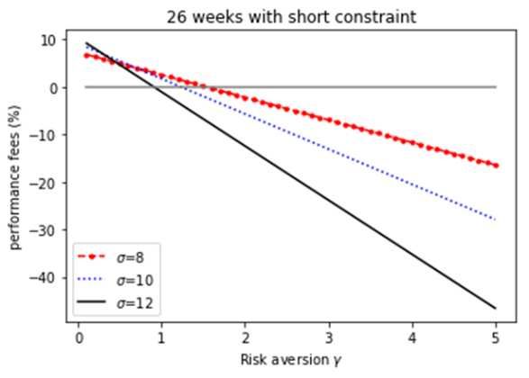
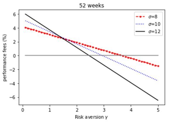
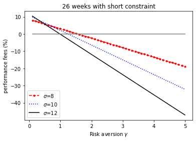
Table 4 presents the impact on the short selling constraint and we see that the SR

for the 26-week predictive model is still higher that that for the benchmark in rows (1),

(4), and (7), while the performance fee is no longer positive. This is because the SR of

the benchmark model increases with the short constraint. Moreover, the performance fee

measure depends upon the investor’s utility in Equation (8) and hence the risk aversion

parameter plays an important role.

4.5. Change in risk aversion

Given the importance of short positions in the cryptocurrency markets, we investigate

whether the risk aversion parameter affects our results. High volatility in the

cryptocurrencies means that the second term of the right-hand side in Equation (8) has a

dominant impact, which implies that our result may have been sensitive to a change in

the risk aversion parameter. Figure 1 depicts the result of the performance fee measure as

changing the risk aversion parameter from 0.1 to 5. The left panel in Figure 1 illustrates

the results for the 26-week rolling window model without the short constraint. We see

that the performance fee measure keeps a positive value over the risk aversion parameter

interval.

 We move on to the result for the 26-week rolling window model with the short

 18

constraint. The right panel in Figure 1 illustrates that the performance fee measure

becomes negative as reaches around 1.5. This decay speed is faster than the result

reported by the exchange rates as in Della Corte et al. (2009), since volatility on the

cryptocurrency portfolio is much larger than that on a currency portfolio. The risk

aversion parameter assumption is substantial whether cryptocurrency investors obtain an

economic gain. Moreover, when the investor’s risk aversion is small, adopting predictive

models is a reasonable decision for investors. This reflects the fact that cryptocurrencies

are speculative assets and that investor’s risk aversion is very low or investors are more

risk lovers (Cheah and Fry, 2015; Baur et al., 2018b; Corbet et al. 2018). We do not

present results for the 52- and 110-week models since they do not outperform the

benchmark model, as reported by Tables 3 and 4.

 Overall, the change in the risk aversion parameter affects the results. We find

that obtaining a positive economic gain depends upon the degree of the risk aversion if

investors are not allowed to hold the short selling positions.

5. Robustness

Having found the effectiveness of using predictive models for cryptocurrency investors,

we investigate the robustness of our findings. More specifically, we conduct: (i) change

 19

in proportionate cost; (ii) inclusion of Ethereum in our portfolio; (iii) change in the risk

aversion parameter for the Ethereum portfolios; (iv) adopting network factors; and (v)

using the elastic-net approach.

5.1. Change in the proportionate cost

In this subsection, we investigate an impact on transaction costs in this subsection. We

used 50 basis points for all cryptocurrency proportionate costs in the previous section

(Lintilhac and Tourin, 2017; Platanakis et al., 2018). Transaction costs depend upon

market states and it may have a large impact on returns (e.g. Burnside et al. 2007). Figure

2 depicts the change in weights on cryptocurrencies when we employ the 26-week

predictive model. The weights on the four cryptocurrencies vary over time, and therefore

the transaction costs are related to the results. We repeat the same exercise using 25 and

100 basis point proportionate costs.

 Table 5 presents whether a change in the proportionate cost impacts our

empirical results, and we only report the results using the predictive models to save space.

Panel A in Table 5 displays that SR increases by about 0.3 with the 25 basis point

proportionate cost and decreases by about 0.6 with the 100 basis point proportionate cost.

The performance fee decreases monotonically with the proportionate cost when we focus

 20

upon the 26 week rolling results.

 Overall, the change in the proportionate cost is related to SR while the impact on

the performance fee measure is marginal, which is associated with both the predictive and

the benchmark models.

5.2. Including Ethereum

We employed the most liquid four cryptocurrencies in Section 4, which is consistent with

Platanakis et al. (2018) and Platanakis and Urquhart (2019). Dash, however, is a relatively

smaller market capitalization compared with the other three cryptocurrencies. We replace

Dash with Ethereum, which is the second largest market capitalization,14 and repeat the

same exercise.

 Table 6 presents that SRs for both 26- and 52-week regression models are slightly

smaller than those of Table 3. The performance fee measure result depends upon the target

volatility level when we focus upon the 26- week rolling window model. The 52-week

model generates the positive performance fee measures since the SR for the benchmark

model is negative.

14
 This value is based upon the market capitalization of August 25, 2020 and obtained by
crypto.com.

 21

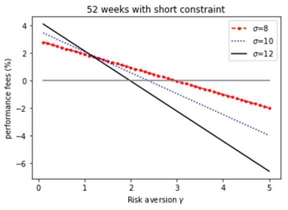
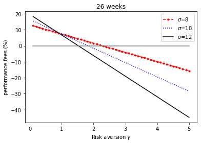
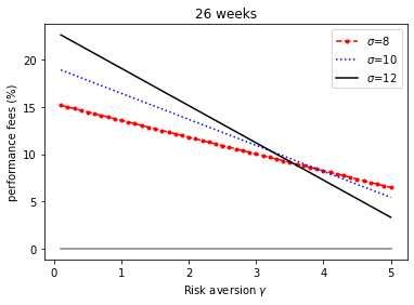
Next, we also consider an impact on the short selling constraint and, interestingly,

SRs for both the predictive and benchmark models are improved, as reported in Table 7.

In particular, the benchmark model provides better results than those of Table 6, which

causes the declines in the performance fee measures.

 In summary, the predictive portfolios generate high SRs compared with the

benchmark portfolios, while the results for the performance fee are mixed.

5.3. Change in risk aversion for Ethereum portfolios

Having found the importance of volatility term for the performance fee measure in the

previous section, we explore whether a change in the risk aversion parameter also plays

an important role for the portfolio that including Ethereum.15

 Figure 3 illustrates the relationships between the risk aversion and the

performance fee. We note that an investor does not obtain an economic gain if the risk

aversion parameter is above 2 with the 26-week predictive model. Turning to the 52-week

predictive model, the decay of performance fee measure is slower than that of the 26-

week model, while the performance fee becomes negative with an increase in the risk

aversion parameter. This supports our previous finding that cryptocurrencies are

15 Impacts on the transaction costs are explored in the online Appendix.

 22

speculative assets and hence are preferable for less risk averse investors (e.g. Baur et al.,

2018b).

5.4. Network factors

Valuations of cryptocurrency depend upon transaction demands since users conduct peer-

to-peer transactions on a decentralized digital platform (e.g. Cong et al., 2020; Sockin and

Xiong, 2020). Cryptocurrencies have strong network effects and Liu and Tsyvinsky

(2020) propose the following network factors: the number of active address (address),

those of transaction count (transaction), those of payment count (volume), and a principal

component of these factors (PC). 16 These data are obtained from Blockchain.com. 17

We also consider these factors in our out-of-sample prediction context and calculate out-

 2
of-sample statistics. Table 8 presents that all four factors outperform the benchmark

and most results are statistically significant based upon MSPE-adjusted p-values. The

impacts, however, are moderate in compared with those of Table 2 which use lagged

return information.

5.5. Elastic-net approach

16
 We exclude the number of wallet uses since weekly data is not available. We replace the number
of payment count with trading volumes for data availability.
17 https://www.blockchain.com/charts#currency

 23

This section considers to combine cryptocurrency price and network factor information.

To this end, we employ the elastic-net approach proposed by Zou and Hastie (2005). The

elastic-net is a variable selection method and overcomes the drawback of Lasso

(Tibshirani, 1996) that selects a single variable from a group of correlated variables. It

has been widely used in the asset return and macroeconomic indicator predictions (e.g.

Rapach et al., 2013; Li, Tsiakas, and Wang, 2015). Estimators using the elastic-net are

obtained by the following system:
 2
 
 1 (10)
 arg min = ∑ ( +1 − − ∑ , )
 2
 =1 =1

 s.t. ∑ =1| | < 1 and ∑ =1 2 < 2

where is the number of predictors, 1 and 2 are the tuning parameters. When 1 =

∞, Equation (10) reduces to the ridge regression and when 2 = ∞, Equation (10) does

to the Lasso. We follow Li and Chen (2014) and decide the turning parameters using cross

validation for each window throughout the out-of-sample period. Table A3 shows the out-

 2
of-sample statistic results and we observe that the combination between legged

returns and network factors does not lead to prediction accuracy. We conclude that the

lagged returns are strong predictors for cryptocurrency returns at weekly frequencies.

 24

6. Conclusion

This study evaluates predictability for cryptocurrency returns using the dynamic

allocation approach proposed by Della Corte et al. (2009). Cryptocurrency markets are

expanding rapidly and many investors are attracted due to the high risk and return profile.

The cryptocurrency markets have not yet matured and some studies report that

information efficiency is not satisfied (Urquhart, 2016; Tran and Leirvik, 2020). There is

no fundamental value for cryptocurrencies and many investors are speculators, causing

bubble periods (Cheah and Fry, 2015; Baur et al., 2018b). These features of the

cryptocurrency markets imply that investors may obtain profits using past price

information (Grosby et al. 2020). Moreover, a cryptocurrency return is not strongly

correlated to the returns of other cryptocurrencies (Klein et al. 2018), and hence adopting

the portfolio approach provides diversification benefits with investors.

 We find the following results. First, the forecast model for each cryptocurrency

outperforms the historical average benchmark model in the out of sample context. Second,

our cryptocurrency portfolios constructed by the forecast models generate a higher SR

than that of the benchmark and the difference between SRs is statistically significant.

Third, an investor obtains an economic gain around 12% per week when he or she

switches from the benchmark portfolio to the predictive model portfolio. Fourth, a change

 25

in the investor’s risk aversion impacts the economic gain. In particular, the result is

sensitive to the change in the investor’s risk aversion with the short selling constraint.

This contrast result to the exchange rate literature reflects high volatility on the

cryptocurrencies.

References

Ahmed, S., Liu; X., and Valente, G. (2016). Can currency-based risk factors help forecast
exchange rates?” International Journal of Forecasting, 32, 75-97.

Barroso, P. and Santa-Clara, P. (2015). Beyond the carry trade: optimal currency
portfolios. Journal of Financial and Quantitative Analysis, 50, 1037-1056.

Baur, D.G., Dimpfl, T., and Konstantin, K. (2018a). Bitcoin, gold and the US dollar – A
replication and extension. Finance Research Letters, 25, 103-110.

Baur, D.G., Hong, K. and Lee., A.D. (2018b). Bitcoin: medium of exchange or speculative
assets? Journal of International Financial Markets, Institutions and Money, 54, 177-189.

Benartzi, S. and Thaler, R.H. (1995). Myopic loss aversion and the equity premium puzzle.
Quarterly Journal of Economics, 110, 73-92.

Biais, B., Bisière, C., Bouvard, M., Casamatta, C., and Menkveld, A.J. (2020).
Equilibrium bitcoin pricing. EconPol Working Paper 45.

Bleher, J. and Dimpfl, T. (2019). Today I got a million, tomorrow, I don't know: On the
predictability of cryptocurrencies by means of Google search volume. International
Review of Financial Analysis, 63,147-159.

Bouoiyour, J., Selmi, R., Tiwari, A., and Olayeni, O. (2016). What drives Bitcoin price?
Economics Bulletin, 36, 843-850.

 26

Brière, M., Oosterlinck, K., and Szafarz, A. (2015). Virtual currency, tangible return:
Portfolio diversification with Bitcoin. Journal of Asset Management, 16, 365-373.

Burnside, C., Eichenbaum, M., Rebelo, S., 2007. The returns to currency speculation in
emerging markets. American Economic Review, Papers and Proceedings, 97, 333–338

Campbell, J.Y. and Cochrane, J.H. (1999). By force of habit: A consumption based
explanation of aggregate stock market behavior. Journal of Political Economy, 107, 205-
251.

Campbell, J.Y. and Thompson, S.B. (2008). Predicting excess stock returns out of sample:
Can anything beat the historical average? Review of Financial Studies, 21, 1509-1531.

Cheah, E-T. and Fry, J. (2015). Speculative bubbles in Bitcoin markets? An empirical
investigation into the fundamental value of Bitcoin. Economics Letters, 130, 32-36.

Chu, J., Zhang, Y., and Chan, S. (2019). The adaptive market hypothesis in the high
frequency cryptocurrency market. International Review of Financial Analysis, 64, 221-
231.

Ciaian, P., Rajcaniova, M., and Kancs, A. (2018). Virtual relationships: Short- and long-
run evidence from BitCoin and altcoin markets. Journal of International Financial
Markets, Institutions and Money, 52, 173-195.

Clark, T. and West, K. (2007). Approximately normal tests for equal predictive accuracy
in nested models. Journal of Econometrics, 138, 291-311.

Cong, L.W., Li, Y., and Wang, N. (2020). Tokenomics: dynamic adoption and valuation.
Review of Financial Studies, forthcoming.

Corbet, S., Lucey, B., Urquhart, A., and Yarovaya, L. (2019). Cryptocurrencies as a
financial asset: A systematic analysis. International Review of Financial Analysis,
62,182-199.

Corbet, S., Lucey, B., and Yarovaya, L. (2018). Datestamping the Bitcoin and Ethereum
bubbles. Finance Research Letters, 26, 81-88.

 27

Della Corte, P., Sarno, L., and Tsiakas, I. (2009). An economic evaluation of empirical
exchange rate models. Review of Financial Studies, 22, 3491-3530.

Della Corte, P., Sarno, L., and Tsiakas, I. (2011). Spot and forward volatility in foreign
exchange. Journal of Financial Economics, 100, 496-513.

Diebold, F.X., and Mariano, R.S. (1995). Comparing predictive accuracy. Journal of
Business and Economic Statistics, 13, 253–63.

Dyhrberg, A.H. (2016). Bitcoin, gold and the dollar – A GARCH volatility analysis.
Finance Research Letters, 16, 85-92.

Fang, L., Bouri, E., Gupta, R., and Roubaud, D. (2019). Does global economic uncertainty
matter for the volatility and hedging effectiveness of Bitcoin? International Review of
Financial Analysis, 61, 29-36.

Fama, E.F. and French, K.R. (1993). Common risk factors in the returns on stock and
bonds. Journal of Financial Economics, 33, 3–56.

Fleming, J., Kirby, C., and Ostdiek, B. (2001). The economic value of volatility timing.
Journal of Finance, 56, 329-352.

Fry, J. and Cheah, E.-T. (2016). Negative bubbles and shocks in cryptocurrency markets.
International Review of Financial Analysis, 47, 343-352.

Gandelman, N. and Hernandez-Murillo, R. (2015). Risk aversion at the country
level. Review, 97, 53-66.

Griffin, J.M. and Shams, A. (2020). Is Bitcoin really untethered? Journal of Finance, 75,
1913-1964.

Grobys, K., Ahmed, S., and Sapkota, N. (2020). Technical trading rules in the
cryptocurrency market. Finance Research Letters, 32, 101396.

Guesmi, K., Saadi, S., Abid, I., and Ftiti, Z. (2019). Portfolio diversification with virtual
currency: Evidence from bitcoin. International Review of Financial Analysis, 63, 431-

 28

437.

Kajtazi, A. and Moro, A. (2019). The role of bitcoin in well diversified portfolios: A
comparative global study. International Review of Financial Analysis, 61, 143-157.

Keim, D.B. and Stambaugh, R.F. (1984). A Further Investigation of the Weekend Effect
in Stock Returns. Journal of Finance, 39, 819-835.

Klein, T., Thu, H.P., and Walther, T. (2018). Bitcoin is not the new gold - a comparison of
volatility, correlation, and portfolio performance. International Review of Financial
Analysis, 59, 105-116.

Kristoufek, L., (2015). What are the main drivers of the Bitcoin price? Evidence from
wavelet coherence analysis. PLOS One, 10, e0123923.

Ledoit, O. and Wolf, M. (2008). Robust performance hypothesis testing with the Sharpe
ratio. Journal of Empirical Finance, 15, 850–859.

Li, J. and Chen, W. (2014). Forecasting macroeconomic time series: LASSO-based
approaches and their forecast combinations with dynamic factor models. International
Journal of Forecasting, 30, 996-1015.

Li, J., Tsiakas I., and Wang, W. (2015). Predicting exchange rates out of sample: can
economic fundamentals beat the random walk? Journal of Financial Econometrics, 13,
293-341.

Li, X and Wang, C.A. (2017). The technology and economic determinants of
cryptocurrency exchange rates: The case of Bitcoin. Decision Support System, 95, 49-60.

Lintilhac, P.S. and Tourin, A. (2017). Model-based pairs trading in the bitcoin markets.
Quantitative Finance, 17, 703–716.

Liu, Y. and Tsyvinski, A. (2020). Risks and returns of cryptocurrency, Review of
Financial Studies, Forthcoming.

Mehra, R and Prescott, E. C. (1985). The equity premium: A puzzle. Journal of Monetary
Economics, 15, 145-161.

 29

Nadarajah, S. and Chu, J. (2017). On the inefficiency of Bitcoin. Economics Letters, 150,
6-9.

Opie, W. and Riddiough, S.J. (2020). Global currency hedging with common risk factors.
Journal of Financial Economics, Forthcoming.

Philippas, D., Philippas, N., Tziogkidis, P., and Rjiba, H. (2020). Signal-herding in
cryptocurrencies. Journal of International Financial Markets, Institutions and Money,
Forthcoming.

Platanakis, E., Sutcliffe, C., and Urquhart, A. (2018). Optimal vs naïve diversification in
cryptocurrencies. Economics Letters, 171, 93-96.

Platanakis, E. and Urquhart, A. (2019). Portfolio management with cryptocurrencies: The
role of estimation risk. Economics Letters, 177, 76-80.

Rapach, D.E., Strauss, J.K., and Zhou, G. (2010). Out-of-Sample Equity Premium
Prediction: Combination Forecasts and Links to the Real Economy. Review of Financial
Studies, 23, 821-861.

Rapach, D.E., Strauss, J.K., and Zhou, G. (2013). International Stock Return
Predictability: What Is the Role of the United States? Journal of Finance, 68, 1633-1662.

Rime, D., Sarno, L., and Sojli, E. (2010). Exchange rate forecasting, order flow and
macroeconomic information. Journal of International Economics, 80, 72-88.
Risse, M. (2019). Combining wavelet decomposition with machine learning to forecast
gold returns. International Journal of Forecasting, 35, 601-615.

Rognone, L., Hyde, S., and Zhang, S.S. (2020). News sentiment in the cryptocurrency
market: An empirical comparison with Forex. International Review of Financial Analysis,
69, 101462.

Schilling, L. and Uhlig, H. (2019). Some simple bitcoin economics. Journal of Monetary
Economics, 106, 16-26.

Shen, D., Urquhart, A., and Wang, P. (2019). Does twitter predict Bitcoin? Economics
Letters, 174, 118-122.

 30

Sockin, M. and Xiong, W. (2020). A model of cryptocurrencies. NBER Working Papers
26816.

Thornton, D.L. and Valente, G. (2012). Out-of-sample predictions of bond excess returns
and forward rates: an asset allocation perspective. Review of Financial Studies, 25, 3141-
3168.

Tibshirani, R. (1996). Regression Shrinkage and Selection via the Lasso. Journal of the
Royal Statistical Society, Series B(Methodological), 58, 267-288.

Tran, V.L. and Leirvik, T. (2020). Efficiency in the markets of crypto-currencies. Finance
Research Letters, 35, 101382.

Urquhart, A. (2016). The inefficiency of Bitcoin. Economics Letters, 148, 80-82.

Welch, I. and Goyal, A. (2008), A comprehensive look at the empirical performance
Of equity premium prediction. Review of Financial Studies, 21, 1455-1508.

West, K.D. (1996). Asymptotic inference about predictive ability. Econometrica, 64,
1067–84.

Zimmerman, P. (2020). Blockchain structure and cryptocurrency prices. Bank of England
Staff Working Paper No. 855

Zou, H. and Hastie, T. (2005). Regularization and variable selection via the elastic net,
Journal of the Royal Statistical Society, Series B(Statistical Methodology), 67, 301–320

 31

Table 1 Summary statistics of cryptocurrency returns
 Mean Std Dev Skewness Kurtosis Max Min SR
Bitcoin 1.44 10.70 -0.23 5.34 36.83 -41.23 0.95
Litecoin 1.01 16.07 2.18 15.24 110.37 -36.38 0.44
Ripple 1.31 19.86 2.55 14.32 125.81 -47.15 0.47
Dash 1.27 16.38 1.62 9.25 91.61 -37.98 0.55
Ethereum 2.15 17.50 1.05 6.40 80.45 -52.88 0.88
Notes: This table reports mean, standard deviations, skewness, kurtosis, maximum,
minimum, and the annualized Sharpe ratio of cryptocurrency returns. A one-month
Treasury bill rate is used as the risk-free rate in order to calculated the Sharpe ratio. We
employ weekly returns and the sample period covers from 12th July, 2015 to 29th July,
2020.

 32

2
 Table 2 Out-of-sample forecasting results
 Bitcoin Litecoin Ripple Dash Ethereum
 (1) 26 weeks 21.26 *** 12.82 *** 41.30 *** 20.06 *** 22.02 ***
 (2) 52 weeks 10.38 *** 7.75 ** 21.76 ** 11.04 ** 12.38 ***
 (3) 110 weeks 1.30 ** 0.68 2.04 3.62 ** -0.10

Notes: This table displays statistical measures of the out-of-sample forecast of predictive
models in Equation (1). We conduct the one-week-ahead return forecasts of
cryptocurrencies using rolling regressions. Predictors are from one to four-week lagged
returns and the window sizes are 26, 52 and 110 weeks. The Campbell and Thompson
 2
(2008) out-of-sample statistic is reported, and the p-value based upon the Clark and
West (2007) MSPE-adjusted statistic is employed: the statistic corresponds to a one-side
test of the null hypothesis that the competing model has equal MSPE relative to the
historical average benchmark forecasting model against the alternative hypothesis that
the competing forecasting model has a lower MSPE than the historical average
benchmark forecasting model. *,**, and *** indicate significance at the 10%, 5% and 1%
levels, respectively.

 33

Table 3 Out-of-sample portfolio return predictability
 Benchmark Predictive
Panel A: σP =8 Mean St.Dev SR Mean St.Dev SR Φ
 (1) 26 weeks -0.22 7.99 -0.03 7.76 8.08 0.96 * 11.80
 (2) 52 weeks 2.77 8.20 0.34 2.15 8.19 0.26 -0.61
 (3) 110 weeks -2.60 8.04 -0.32 -6.01 7.69 -0.78 -119.02
Panel B: σP =10
 (4) 26 weeks 0.04 9.98 0.00 10.02 10.11 0.99 * 13.68
 (5) 52 weeks 3.82 10.24 0.37 3.04 10.23 0.30 -0.58
 (6) 110 weeks -2.81 10.05 -0.28 -7.07 9.60 -0.74 -183.57
Panel C: σP =12
 (7) 26 weeks 0.31 11.97 0.03 12.28 12.13 1.01 * 15.14
 (8) 52 weeks 4.87 12.29 0.40 3.93 12.27 0.32 -0.47
 (9) 110 weeks -3.02 12.06 -0.25 -8.14 11.52 -0.71 -262.12

Notes: This table presents the out-of-sample economic value of the predictive models for
cryptocurrency portfolio returns, including the historical average benchmark model. We
conduct the one-week-ahead return forecasts of cryptocurrencies using rolling regressions
The window sizes are 26, 52 and 110 weeks. We employ four cryptocurrencies: Bitcoin,
Litecoin, Ripple and Dash. Mean is the annualized returns and St.Dev is the annualized
standard deviation on the portfolio. SR indicates the annualized Sharpe ratio (SR) and the
SR difference between the benchmark and the predictive models are tested by the method
of Ledoit and Wolf (2008). The weekly performance fee measure (Φ) for the predictive
model against the benchmark model is calculated by Equation (9). We set the portfolio
target volatility ( ∗ ) to 8%, 10% and 12%, respectively. The relative risk aversion
parameter is 2 (Della Corte et al., 2009). *,**, and *** indicate significance at the
10%, 5% and 1% levels, respectively.

 34

Table 4 Out-of-sample portfolio return predictability with the short constraint
 Benchmark Predictive
Panel A: σP =8 Mean St.Dev SR Mean St.Dev SR Φ
 (1) 26 weeks 1.52 5.69 0.27 5.96 6.17 0.97 * -2.44
 (2) 52 weeks 3.25 6.20 0.52 3.01 6.18 0.49 0.20
 (3) 110 weeks -1.31 6.50 -0.20 -3.67 5.61 -0.66 -64.73
Panel B: σP =10
 (4) 26 weeks 2.22 7.11 0.31 7.77 7.71 1.01 * -6.46
 (5) 52 weeks 4.41 7.74 0.57 4.11 7.72 0.53 0.46
 (6) 110 weeks -1.20 8.13 -0.15 -4.15 7.01 -0.59 -99.36
Panel C: σP =12
 (7) 26 weeks 2.92 8.53 0.34 9.58 9.25 1.04 * -11.84
 (8) 52 weeks 5.58 9.29 0.60 5.22 9.26 0.56 0.79
 (9) 110 weeks -1.09 9.75 -0.11 -4.64 8.41 -0.55 -141.43

Notes: This table presents the out-of-sample economic value of the predictive models for
cryptocurrency portfolio returns, including the historical average benchmark model.
Portfolios are constructed without short positions. We conduct the one-week-ahead return
forecasts of cryptocurrencies using rolling regressions. The window sizes are 26, 52 and
110 weeks. We employ four cryptocurrencies: Bitcoin, Litecoin, Ripple and Dash. Mean
is the annualized returns and St.Dev is the annualized standard deviation on the portfolio.
SR indicates the annualized Sharpe ratio (SR) and the SR difference between the
benchmark and the predictive models are tested by the method of Ledoit and Wolf (2008).
The weekly performance fee measure (Φ) for the predictive model against the benchmark
model is calculated by Equation (9). We set the portfolio target volatility ( ∗ ) to 8%, 10%
and 12%, respectively. The relative risk aversion parameter is 2 (Della Corte et al.,
2009). *,**, and *** indicate significance at the 10%, 5% and 1% levels, respectively.

 35

Table 5 Impacts on transaction costs
Panel A: without short constraint
 TC=25 TC=50 TC=100
Panel A: σP=8 Mean St.Dev SR Φ Mean St.Dev SR Φ Mean St.Dev SR Φ
 (1) 26 weeks 10.30 8.06 1.28 12.00 7.76 8.08 0.96 11.80 2.66 8.16 0.33 11.68
 (2) 52 weeks 4.48 8.19 0.55 0.19 2.15 8.19 0.26 -0.61 -2.52 8.19 -0.31 -2.10
Panel B: σP=10
 (3) 26 weeks 13.20 10.07 1.31 13.91 10.02 10.11 0.99 13.68 3.64 10.21 0.36 13.66
 (4) 52 weeks 5.96 10.24 0.58 0.51 3.04 10.23 0.30 -0.58 -2.80 10.23 -0.27 -2.61
Panel C: σP=12
 (5) 26 weeks 16.10 12.09 1.33 15.39 12.28 12.13 1.01 15.14 4.63 12.25 0.38 15.27
 (6) 52 weeks 7.44 12.28 0.61 0.94 3.93 12.27 0.32 -0.47 -3.08 12.28 -0.25 -3.11

Panel B: with short constraint
 TC=25 TC=50 TC=100
Panel A: σP=8 Mean St.Dev SR Φ Mean St.Dev SR Φ Mean St.Dev SR Φ
 (7) 26 weeks 7.39 6.17 1.20 -2.21 5.96 6.17 0.97 -2.44 3.11 6.18 0.50 -2.74
 (8) 52 weeks 4.12 6.18 0.67 0.83 3.01 6.18 0.49 0.20 0.78 6.17 0.13 -0.93
Panel B: σP=10
 (9) 26 weeks 9.56 7.71 1.24 -6.29 7.77 7.71 1.01 -6.46 4.20 7.72 0.54 -6.67
 (10) 52 weeks 5.51 7.73 0.71 1.38 4.11 7.72 0.53 0.46 1.33 7.71 0.17 -1.20
Panel C: σP=12
 (11) 26 weeks 11.73 9.25 1.27 -11.73 9.58 9.25 1.04 -11.84 5.30 9.26 0.57 -11.90
 (12) 52 weeks 6.89 9.27 0.74 2.08 5.22 9.26 0.56 0.79 1.88 9.25 0.20 -1.48

Notes: This table presents the out-of-sample economic value of the predictive models for
cryptocurrency portfolio returns. We set the proportionate cost to 25, 50 and 100 basis
points in order to calculated the transaction costs (TC). TC=50 is employed in Tables 3
and 4. Panel A presents the results without the short constraint and Panel B does the
results with the short constraint. The window sizes are 26 and 52 weeks. We employ four
cryptocurrencies: Bitcoin, Litecoin, Ripple and Dash. Mean is the annualized returns and
St.Dev is the annualized standard deviation on the portfolio. SR indicates the annualized
Sharpe ratio (SR) and the SR difference between the benchmark and the predictive models
are tested by the method of Ledoit and Wolf (2008). The weekly performance fee measure
(Φ) for the predictive model against the benchmark model is calculated by Equation (9).
We set the portfolio target volatility ( ∗ ) to 8%, 10% and 12%, respectively. The relative
risk aversion parameter is 2 (Della Corte et al., 2009).

 36

Table 6 Out-of-sample portfolio return predictability: Ethereum
 Benchmark Predictive
Panel A: σP=8 Mean St.Dev SR Mean St.Dev SR Φ
 (1) 26 weeks -0.31 7.92 -0.04 6.50 8.28 0.79 1.59
 (2) 52 weeks -2.48 8.02 -0.31 -0.32 8.09 -0.04 0.75
Panel B: σP=10
 (3) 26 weeks -0.07 9.90 -0.01 8.45 10.35 0.82 -1.57
 (4) 52 weeks -2.75 10.02 -0.27 -0.04 10.11 0.00 1.66
Panel C: σP=12
 (5) 26 weeks 0.17 11.87 0.01 10.40 12.42 0.84 -6.16
 (6) 52 weeks -3.01 12.02 -0.25 0.23 12.13 0.02 1.16

Notes: This table presents the out-of-sample economic value of the predictive models for
cryptocurrency portfolio returns, including the historical average benchmark model. We
conduct the one-week-ahead return forecasts of cryptocurrencies using rolling regressions.
The window sizes are 26 and 52 weeks. We employ four cryptocurrencies: Bitcoin,
Litecoin, Ripple and Ethereum. Mean is the annualized returns and St.Dev is the
annualized standard deviation on the portfolio. SR indicates the annualized Sharpe ratio
(SR) and the SR difference between the benchmark and the predictive models are tested
by the method of Ledoit and Wolf (2008). The weekly performance fee measure (Φ) for
the predictive model against the benchmark model is calculated by Equation (9). We set
the portfolio target volatility ( ∗ ) to 8%, 10% and 12%, respectively. The relative risk
aversion parameter is 2 (Della Corte et al., 2009). *,**, and *** indicate significance
at the 10%, 5% and 1% levels, respectively.

 37

Table 7 Out-of-sample portfolio return predictability:
 Ethereum and the short constraint
 Benchmark Predictive
Panel A: σP=8 Mean St.Dev SR Mean St.Dev SR Φ
 (1) 26 weeks 2.17 6.00 0.36 5.99 6.39 0.94 -2.17
 (2) 52 weeks 1.03 6.12 0.17 2.53 6.21 0.41 0.92
Panel B: σP=10
 (3) 26 weeks 3.04 7.50 0.41 7.80 7.99 0.98 -5.66
 (4) 52 weeks 1.65 7.65 0.22 3.51 7.76 0.45 0.55
Panel C: σP=12
 (5) 26 weeks 3.91 8.99 0.43 9.62 9.58 1.00 -10.33
 (6) 52 weeks 2.26 9.18 0.25 4.50 9.31 0.48 -0.06

Notes: This table presents the out-of-sample economic value of the predictive models for
cryptocurrency portfolio returns, including the historical average benchmark model.
Portfolios are constructed without short positions. We conduct the one-week-ahead return
forecasts of cryptocurrencies using rolling regressions. The window sizes are 26 and 52
weeks. We employ four cryptocurrencies: Bitcoin, Litecoin, Ripple and Ethereum. Mean
is the annualized returns and St.Dev is the annualized standard deviation on the portfolio.
SR indicates the annualized Sharpe ratio (SR) and the SR difference between the
benchmark and the predictive models are tested by the method of Ledoit and Wolf (2008).
The weekly performance fee measure (Φ) for the predictive model against the benchmark
model is calculated by Equation (9). We set the portfolio target volatility ( ∗ ) to 8%, 10%
and 12%, respectively. The relative risk aversion parameter is 2 (Della Corte et al.,
2009).

 38

2
 Table 8 Out-of-sample forecasting results: network factors
 Bitcoin Litecoin Ripple Dash Ethereum
Panel A: address
 (1) 26 weeks 6.88 *** 3.48 *** 3.78 *** 5.42 ** 6.15 **
 (2) 52 weeks 2.03 * 1.41 * 1.56 * 1.46 1.56 *
Panel B: transaction
 (3) 26 weeks 5.03 ** 7.44 *** 5.46 ** 5.30 *** 5.07 ***
 (4) 52 weeks 1.82 ** 2.34 * 3.46 1.82 ** 2.78 **
Panel C: volume
 (5) 26 weeks 4.05 *** 5.96 *** 6.45 *** 4.70 *** 5.68 ***
 (6) 52 weeks 3.35 *** 4.59 *** 4.04 *** 2.12 *** 3.32 ***
Panel D: PC
 (7) 26 weeks 5.83 *** 2.67 * 6.87 *** 5.48 *** 5.84 ***
 (8) 52 weeks 2.89 ** 5.48 * 4.27 ** 6.10 *** 5.01 ***

Notes: This table displays statistical measures of the out-of-sample forecast of predictive
models in Equation (1). We consider the following four network factors as predictors (Liu
and Tsyvinsky, 2020): the number of active address (address), those of transaction count
(transaction), trading volumes (volume), and a principal component of these factors (PC).
We conduct the one-week-ahead return forecasts of cryptocurrencies using rolling
regressions. The window sizes are 26 and 52 weeks. The Campbell and Thompson (2008)
 2
out-of-sample statistic is reported, and the p-value based upon the Clark and West
(2007) MSPE-adjusted statistic is employed: the statistic corresponds to a one-side test
of the null hypothesis that the competing model has equal MSPE relative to the historical
average benchmark forecasting model against the alternative hypothesis that the
competing forecasting model has a lower MSPE than the historical average benchmark
forecasting model. *,**, and *** indicate significance at the 10%, 5% and 1% levels,
respectively.

 39

Figure 1. Risk aversion and performance fee measure

Notes: This figure provides the relationships between the risk aversion parameter ( ) and
the performance fee measure (Φ). The left figure presents the 26-week rolling regression,
the right figure does the 26-week rolling regression with the short constraint. We employ
four cryptocurrencies: Bitcoin, Litecoin, Ripple and Dash. We set the portfolio target
volatility ( ∗ ) to 8%, 10% and 12%, respectively.

 40

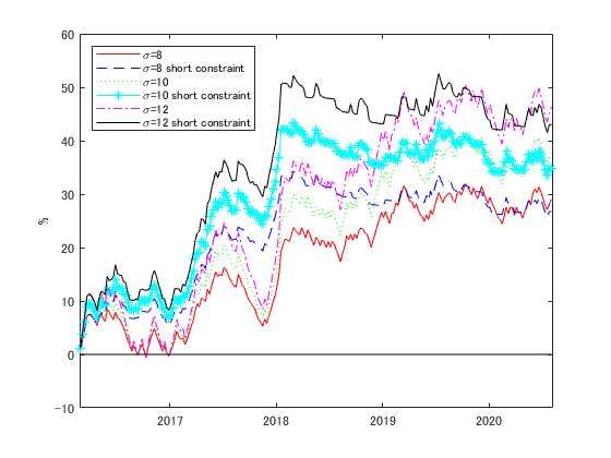
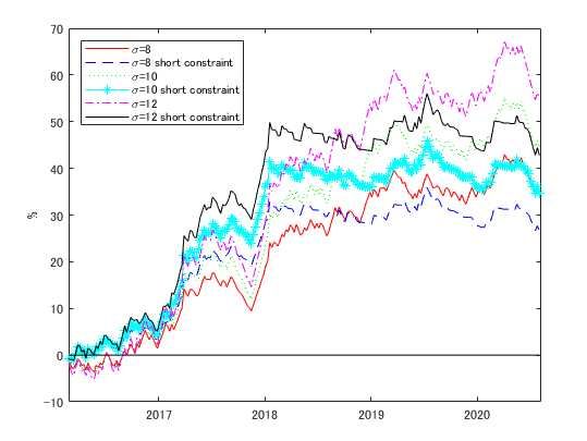
Figure 2. Weights on cryptocurrencies

Notes: This figure provides weights on cryptocurrencies based upon the predictive models.
We employ the 26-week rolling regressions and the weights are determined by Equation
(4). We use four cryptocurrencies: Bitcoin, Litecoin, Ripple and Dash. The upper left
panel sets the target volatility to 8%, the upper right panel does that to 10% and the lower
panel does that to 12%. We do not impose the short constraint.

 41

Figure 3. Risk aversion and performance fee measure: Ethereum

Notes: This figure provides the relationships between the risk aversion parameter ( ) and
the performance fee measure (Φ ). The upper left figure presents the 26-week rolling
regression, the upper right figure does the 26-week rolling regression with the short
constraint, the lower left figure does the 52-week rolling regression and the lower right
figure does the 52-week rolling regression with the short. We employ four
cryptocurrencies: Bitcoin, Litecoin, Ripple and Ethereum. We set the portfolio target
volatility ( ∗ ) to 8%, 10% and 12%, respectively.

 42