A FOM/ROM HYBRID APPROACH FOR ACCELERATING NUMERICAL SIMULATIONS - MPG.PURE
←
→
Page content transcription
If your browser does not render page correctly, please read the page content below
A FOM/ROM Hybrid Approach for Accelerating Numerical
                                                                                                               ∗
                                                                                          Simulations
                                                                                    †1                   ‡2                     §3
                                                                    Lihong Feng          , Guosheng Fu        , and Zhu Wang
arXiv:2103.08642v1 [math.NA] 15 Mar 2021

                                           1
                                               Max Planck Institute for Dynamics of Complex Technical Systems, 1 Sandtorstr, 39106
                                                                              Magdeburg, Germany
                                               2
                                                 Department of Applied and Computational Mathematics and Statistics, University of
                                                                       Notre Dame, Notre Dame, IN 46556
                                                 3
                                                   Department of Mathematics, University of South Carolina, Columbia, SC 29208

                                                                                              Abstract

                                                       The basis generation in reduced order modeling usually requires multiple high-fidelity large-
                                                   scale simulations that could take a huge computational cost. In order to accelerate these
                                                   numerical simulations, we introduce a FOM/ROM hybrid approach in this paper. It is devel-
                                                   oped based on an a posteriori error estimation for the output approximation of the dynamical
                                                   system. By controlling the estimated error, the method dynamically switches between the
                                                   full-order model and the reduced-oder model generated on the fly. Therefore, it reduces the
                                                   computational cost of a high-fidelity simulation while achieving a prescribed accuracy level.
                                                   Numerical tests on the non-parametric and parametric PDEs illustrate the efficacy of the
                                                   proposed approach.

                                           Keywords. Reduced-order model, proper orthogonal decomposition, error estimation

                                           1       Introduction

                                           Reduced order modeling has been developed to provide an efficient computational model for
                                           dynamical systems appeared in many scientific research and engineering application problems.
                                               ∗
                                                The authors acknowledge the support from the Institute for Computational and Experimental Research in
                                           Mathematics (ICERM) at Brown University for participating the “Model and dimension reduction in uncertain
                                           and dynamic systems” semester program in Spring 2020, which were supported by the National Science Foundation
                                           under Grant No. DMS-1439786 and the Simons Foundation Grant No. 50736. Z. Wang was partially supported by
                                           the National Science Foundation through Grants No. DMS-1913073,2012469 and the U.S. Department of Energy
                                           Grant No. DE-SC0020270.
                                              †
                                                E-mail: feng@mpi-magdeburg.mpg.de
                                              ‡
                                                E-mail: gfu@nd.edu
                                              §
                                                E-mail: wangzhu@math.sc.edu; Corresponding author

                                                                                                  1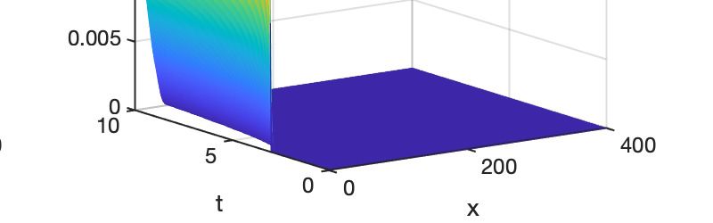
Given a parametric, time-dependent problem, the projection-based model reduction method first
generates reduced basis at an offline stage from snapshots obtained at selected parameters and
time instances, and builds a low-dimensional model in which the matrices and vectors of the
system can be fully assembled; then at the online stage, this reduced-order model (ROM) can
be simulated at a very low cost, thus make fast or even real-time numerical simulations feasible
for many-query applications. Model reduction techniques have achieved many successes, but also
faces several issues.

    On the one hand, to build ROMs for a complex system, one usually has to run large-scale, high
fidelity simulations for many times to find the reduced basis. Although the basis generation is part
of the offline process, its high computational effort makes reduced order modeling not attractive
in practice. Thus, it is desired to speed up this offline process. On the other hand, it is difficult
to build effective ROMs for certain problems. For instance, if problems with a large Kromogrov
n-width are considered such as transport or convection-dominated phenomena, it is generally hard
to find a low-dimensional basis for approximating the solution manifold. Meanwhile, problems
with varying initial conditions or forcing can bring big challenges to the ROM as well because it is
impossible to parametrize the general initial condition or the forcing, and snapshots are not likely
to cover all the possible system responses. This also makes the prediction ability of ROMs pretty
weak: if the snapshots are collected over a given time interval, once the ROM evolves beyond the
interval, there is no accuracy guarantee of the reduced-order simulations.

    Several approaches have been pursued to tackle these issues. To save the computational cost
for snapshot generation, a hybrid snapshot simulation methodology was proposed to accelerate
the high-quality data generation for the proper orthogonal decomposition (POD) ROM develop-
ment in [3, 2]. In this approach, the simulation alternates between full-order model (FOM) and
local ROM based on criteria related to the singular value distribution and the magnitude of POD
basis coefficients. Similarly, the equation-free/Galerkin-free approaches developed in [7, 21] also
chose between the fine-scale and coarse-scale models during the simulations. The fine-scale run
provides data by performing full-order simulations with a small time step size that finds a handful
of leading POD basis. The POD modes are used to parametrize the low-dimensional attracting
slow manifold; while the coarse-scale run evolves the coefficients of leading POD basis functions
by using a larger step size. The resulting reduced-order approximation can be constructed accord-
ingly, which then initializes the fine-scale simulations. However, the choice of the frequency for
switching between the two scale models is empirical. Note that the idea combining the ROM and
FOM has been used in parallel-in-time simulations, for example, in [9, 6, 17], where the ROM on
the fly is regarded as a coarse propagator. For problems with large Kromogrov n-width, the idea
of adaptivity has been introduced for adjusting reduced basis dynamically. The adaptive h-refined
POD was developed in [4, 8]. In this approach, an adjoint-based error estimation is used to mark
basis vectors with major error contributions. Such basis vectors are then refined till the estimated
error becomes under a prescribed tolerance. The refined basis will be compressed online if the
refined-basis dimension exceeds a specified threshold or a prescribed number of time steps has
elapsed. An online adaptive bases and adaptive sampling was developed for transport-dominated

                                                 2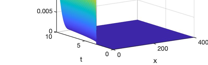
problems in [19], in which both the state and the nonlinear term are projected onto the POD
basis subspace, and the existing POD basis is adjusted at every step. The basis update is of
low rank that is sought from an optimization problem for minimizing the POD/DEIM projection
error of the nonlinear term. A related approach has been proposed in [13] for Hamiltonian sys-
tems. Another research direction is to consider the data-driven ROMs, which first finds nonlinear
solution manifold by taking advantages of the expression power of deep neural network, and then
builds projection-based or machine learning-based ROMs in the nonlinear manifold, for instance,
in [16, 15, 14, 10, 20, 18].

    In this paper, we focus on the projection-based ROMs and use the POD method for construct-
ing the reduced basis. In order to accelerate the snapshot generation and deal with situations for
which the ROM may be not effective, we propose a FOM/ROM hybrid approach. The main idea
is to dynamically update ROM on the fly and switch simulation between the FOM and the ROM,
which is close to the idea in [7, 21, 3], but we introduce a more rigorous criterion based on an a
posteriori error indicator. By comparing the estimated error with a user-defined tolerance, the
hybrid approach automatically alternates between FOM and ROM while controlling the output
approximation error.

    The rest of the paper is organized as follows. In Section 2, we discuss the a posteriori error
indicator; in Section 3, we introduce the hybrid approach, which is numerically investigated in
Section 5. A few concluding remarks are drawn in the last section.

2    Error estimation of output approximation

Consider the following discrete input/output dynamical system: given the state xk and input uk
at time tk , to find the output y k+1 that satisfies

                                 E k xk+1 = Ak xk + f (xk ) + B k uk ,                         (2.1a)
                                        k+1      k+1
                                    y         = Cx       .                                     (2.1b)

 The system in (2.1) is regarded as the full-order model (FOM). The first equation of the state may
come from a time-dependent PDE after discretizing the differential operators and state variable
in space and considering an explicit/semi-implicit time-stepping algorithm. In case an implicit
scheme is used for integrating a nonlinear PDE, this equation could appear in the linearized
system during nonlinear iterations. The second equation evaluates the output of the system,
which approximates linear functionals of the PDE solution – quantities of interest of the system.
Naming (2.1a) the primal equation and, to measure and further control the output approximation
error, we follow [5] and consider the following dual problem: to find xk+1
                                                                       du at time tk+1 satisfying

                                          (E k )| xk+1    |
                                                   du = −C .                                     (2.2)

Based on the original system and choices of time step sizes, the coefficient matrices E k , Ak and B k
could vary with time. Here, for simplicity of presentation, we assume that they stay unchanged

                                                     3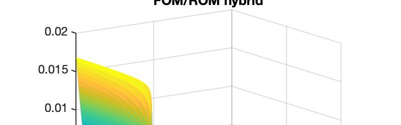
during the simulation in the sequel of discussion. Therefore, we instead consider the following
primal equation:
                                Exk+1 = Axk + f (xk ) + Buk ,                              (2.3)

together with the output equation (2.1b) and the dual equation:

                                                E | xdu = −C | .                                    (2.4)

But we emphasize that our approach could be directly applied to the general case represented by
(2.1) and (2.2).

    To reduce the computational cost of the FOM simulations, model reduction techniques such as
the POD method can be used to generate a ROM. The POD method extracts a low-dimensional
set of orthonormal basis vectors from the snapshot data and uses it to build a low-dimensional
model based on projections. Indeed, given the POD basis Φk and the state xk at time tk , we find
a reduced-order state approximation xbk+1 = Φk xk+1
                                                r   to approximate xk+1 and further determine
a reduced-order output approximation yrk+1 . The associated Galerkin projection-based ROM has
the following form:

                                 Er xk+1
                                     r   = Ar xkr + fr (Φk xkr ) + Br uk ,                         (2.5a)
                                    yrk+1   =   Cr xk+1
                                                    r   ,                                          (2.5b)

 where xkr = Φ|k xk , Er = Φ|k EΦk , Ar = Φ|k AΦk , Br = Φ|k B, Cr = CΦk , and fr (Φk xkr ) =
Φ|k fb(Φk xkr ) with fb(·) = f (·) if POD is used or fb(·) = Pf (·) if an interpolation method is applied.
For instance, when DEIM is considered, P = Φf (P| Φf )−1 P with Φf the DEIM basis and P the
matrix for extracting rows corresponding to the interpolation points.

   The dual equation (2.4) needs to be considered for estimating the error, which has the same
dimension as the FOM. To avoid solving the large-scale discrete system, one can seek an approx-
imate solution x                                                 bdu = Ψk xdu
                 bdu , e.g., via a ROM of the dual equation. Let x         r with Ψk the POD
basis of xdu , the ROM of dual equation reads:
                                                       | |
                                            Er| xdu
                                                 r = −Ψk C .                                        (2.6)

   To derive a bound on the output error, we test (2.4) by xk+1 − x
                                                                  bk+1 and have

                            (xk+1 − x
                                    bk+1 )| E | xdu = −(xk+1 − x
                                                               bk+1 )| C | .                        (2.7)

Taking transpose on both sides yields

                                       bk+1 ) = −x|du E(xk+1 − x
                              C(xk+1 − x                       bk+1 ),                              (2.8)

in which the term on the left represents the output error of the reduced approximation and the
term on right is related to the solution of the dual problem and the residual of the primal problem.
Define
                      k+1                                   (2.3)
                     rpr  := Axk + f (xk ) + Buk − Eb  xk+1 = E(xk+1 − x  bk+1 ),               (2.9)

                                                       4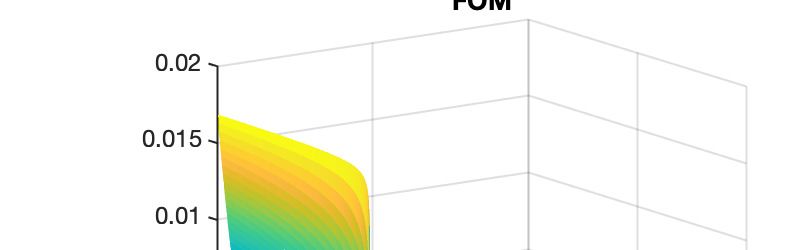
and define the residual of dual equation to be
                                                         (2.4)
                             rdu := −C | − E | x
                                               bdu = E | (xdu − x
                                                                bdu ).                        (2.10)

Therefore, combining (2.8), (2.9) and (2.10), we have

                                                    bk+1 ) = −x|du rpr
                           y k+1 − yrk+1 = C(xk+1 − x               k+1

                                        = [−(x|du − x
                                                    b|du ) − x
                                                             b|du ]rpr
                                                                    k+1                       (2.11)
                                             |
                                        = −(rdu        b|du )rpr
                                                E −1 + x      k+1
                                                                  .

It leads to an upper bound for the output approximation:

                          |y k+1 − yrk+1 | ≤ krdu kkE −1 k + kb
                                                                    k+1
                                                              xdu k krpr k.                   (2.12)

                     k+1 in (2.9) needs the FOM solution xk . To reduce the computational cost,
However, evaluating rpr
            k+1 with the residual of the reduced-order approximation, i.e.,
we replace rpr

                                k+1
                              rbpr      xk + f (b
                                    := Ab       xk ) + Buk − Eb
                                                              xk+1 .                          (2.13)

Then the output error satisfies

                       |y k+1 − yrk+1 | ≤ krdu kkE −1 k + kb
                                                           xdu k ρk+1 kbk+1

                                                                       rpr  k,                (2.14)

where
                                                       k+1 k
                                                     krpr
                                           k+1
                                          ρ      =     k+1
                                                                 .
                                                     kb
                                                      rpr  k
It is proved in [23] that, under mild conditions, e.g., f is bi-Lipschitz continuous, the ratio ρk+1
is bounded by positive constants from above and below. In particular,

              k+1     k+1
            krpr  − rbpr  k = kA(xk − x
                                      bk ) + f (xk ) − f (b
                                                          xk )k ≤ (kAk + Lf )kxk − x
                                                                                   bk k.

When the reduced approximation is accurate enough, i.e., kb  xk − xk k is sufficient small, krpr
                                                                                              k+1 −

  k+1 k becomes close to zero, and the ratio ρk+1 approaches 1. Indeed, this is true in our compu-
rbpr
tational setting presented in the next section, as we aim at finding accurate numerical solutions
by combining the FOM and the ROM during the simulations. Therefore, we define

                              ∆k+1 = krdu kkE −1 k + kb
                                                            k+1
                                                      xdu k kb
                                                             rpr k,                           (2.15)

which gives an error estimation of |y k+1 − yrk+1 | for the system (2.3). We emphasize that ∆k+1
only serves as an error indicator at the step k because the numerical error accumulates over time
that may deflect xk , the initial condition of the very step, off the trajectory of a high-fidelity
simulation.

                                                     5
3 A hybrid approach
Based on the error indicator presented in Section 2, we introduce a FOM/ROM hybrid approach
in this section. The goal is to accelerate numerical simulations while keeping an accurate output
approximations. The basic idea of this approach is to generate a ROM on the fly based on
snapshots available in a fixed-width time window, and apply the ROM whenever possible. The
associated output accuracy is measured by the error indicator ∆k . If it does not reach a user-
defined tolerance, one switches the model to the FOM, updates snapshots, and generates the
ROM that is to be used in the next step’s simulation. Therefore, this approach dynamically
switches the simulation model between the ROM and the FOM. For the system, (2.3) and (2.4),
the approach is detailed in Algorithm 1.
Algorithm 1: The hybrid approach for solving (2.3)-(2.1b)
Input: Initial condition x0 , error tolerance tol, time window width w, total number of time steps nt .
Output: System output.
compute an approximate solution x bdu to the dual equation and evaluate Cdu = krdu kkE −1 k + kbxdu k;
run the FOM from t to t and compute the output; generate snapshots S = [x1 , x2 , . . . , xw ], SE = ES,
1 w
SA = AS and initialize a ROM;
for k = w : nt − 1 do
run the ROM on [tk , tk+1 ], obtain x
bk+1 and evaluate the estimated error ∆k+1 = Cdu kb k+1
rpr k;
k+1
if ∆ ≤ tol then
xk+1 = xbk+1 , flag = 1;
else
solve the FOM for xk+1 ;
set ∆k+1 = eps (in MATLAB notation) and flag = 2.
end
evaluate output y k , update time window data: S, SE and SA ;
if flag = 2 then
generate a ROM based on S, SE and SA .
end
end
Note that here we still assume time invariant coefficient matrices in system (2.3). Since the
dual problem (2.1b) only needs to be solved once, we use a full-order approximation and compute
Cdu = krdu kkE −1 k + kb xdu k at the beginning of the simulation. The hybrid approach starts with
the FOM simulation over a fixed-width time window, [t1 , . . . , tw ]. Based on this time window
data S = [x1 , x2 , . . . , xw ], a ROM is initialized; At each subsequent time step k, we first use the
available ROM to advance the simulation over a step, and evaluate the output error indicator. By
comparing it with a prescribed tolerance (tol), we will either accept the reduced approximation
bk+1 as xk+1 if ∆k+1 ≤ tol, or reject it if ∆k+1 > tol and run a full-order simulation to get xk+1
x
with a higher fidelity. In either case, xk+1 is used to update the time window data S. Whenever
a FOM solution is added, we shall update the ROM.
The computational saving stems from the replacement of FOM with ROM at all the possible
time steps. To determine when to use FOM, the error indicator ∆k+1 is evaluated where the major
6computation is spent on calculating kb k+1 k. For updating the ROMs, the main computation is
rpr
spent on updating the POD basis Φk+1 from S and assembling coefficient matrices and vectors,
Ar , Er and fr , in the reduced system. Note that
k+1
rbpr = AΦk xkr + f (Φk xkr ) + Buk − EΦk xk+1
r ,
and Ar = Φ|k AΦk , Er = Φ|k EΦk , calculating AΦk and EΦk in a cheaper way would improve the
efficiency. On the other hand, the POD basis Φk is generated based on the available time window
snapshots S, which is a tall matrix in general. For such a case, the method of snapshots (MOS)
can be used to find the POD basis (i.e., left singular value vectors of S) quicker than the singular
value decomposition (SVD):
S | SV = V Λ and Φ = SV Λ−1/2 .
The method can be further improved in efficiency as discussed in [22] by taking advantage of
parallel computing. Thus, at the end of the step k in the algorithm, besides updating the time
window snapshots S = [S(:, 2 : w), xk+1 ], we also update SE = [SE (:, 2 : w), Exk+1 ] and SA =
[SA (:, 2 : w), Axk+1 ]. It leads to a cheaper evaluation of
EΦk+1 = SE V Λ−1/2 and AΦk+1 = SA V Λ−1/2
at the next step.
The computational complexity at each step is dominated by the time window data updates
if flag = 1. There, the main complexity, O(n max(r, a)) with r the dimension of ROM and a the
max nonzero numbers in each row of sparse matrices E and A, is used to update time window
data and evaluate error indicator. It generally dominates the cost for solving the reduced system.
When flag = 2, the computational complexity at each step is dominated by the FOM solution
and the ROM update. There, the FOM solution takes O(np ) with p dependent on the choice of
numerical solver, suppose it dominates the nonlinear function evaluation cost O(α(n)), and the
MOS takes O(nw2 +rnw +w3 ), in which O(nw2 ) flops are needed for evaluating S | S, O(w3 ) flops
for the eigen-decomposition of S | S and O(nwr) flops for the calculation of the POD basis. Note
that, when the DEIM is used, additional computation is required for updating the DEIM basis
and interpolation points. Since r ≤ w and w
n in general, the dominating complexity becomes
O(nw2 ). Assume the percentage of the FOM runs in the hybrid model simulation is c × 100%,
for c ∈ [0, 1], then the ratio of the complexity for the FOM to that of the hybrid approach is
np
c(np +nw2 )+(1−c)(n max(r,a))
. Obviously, this factor is bounded by 1c from above and by 1 from below
when w2 ≤ (1 − c)n(p−1) .
The hybrid approach accelerates the FOM simulations, which has several applications: Firstly,
it can be used to speed up the offline snapshot generation for model order reduction (MOR) tech-
niques as it replaces the FOM simulations with the ROM simulations at certain steps; Secondly,
it can overcome the issue on the accuracy loss when using a ROM in a computational setting
different from which the ROM was built. Next, we focus on the first application to illustrate the
usefulness of the approach.
74 Accelerating the offline stage of MOR
The application of ROM usually involves certain high-fidelity simulations to find reduced-order
basis vectors offline and/or update them at the online stages. When the system has a large
dimension, generation of snapshots using the FOM could be time-consuming. In this section we
show that the hybrid approach can be naturally employed at the offline stage of MOR.
In particular, when the reduced basis method (RBM) is applied to parametric time-evolution
problems, the basis to approximate the solution manifold can be found by using the POD-Greedy
algorithm [12]. Guided by an a posteriori error estimator ∆(·), the algorithm implements a
sequence of FOM simulations at selected parameter samples to obtain the corresponding trajectory
of the solution, i.e. the snapshots. At this point, the hybrid simulation in Section 3 can be applied
to accelerating the FOM simulation with accuracy loss being controlled by the error indicator.
In Algorithm 2, we present a modified, hybrid model-based POD-greedy algorithm. It is worth
mentioning that, because the FOM runs occur at a portion of time steps, e.g., {t1 , . . . , tK } in the
hybrid model simulations at µ∗ and the ROMs on the fly are essentially generated from them, one
only needs to collect the snapshots Xµ∗ at those steps, that are enough to represent the system
information.
Algorithm 2: The hybrid model-based POD-Greedy algorithm
Input: Parameter training set Θ, tolerance tol.
Output: basis matrix Φ.
Initialize Φ = [ ], randomly choose µ∗ ∈ Θ;
while ∆(µ∗ ) > tol do
simulate the hybrid model at µ∗ and obtain snapshots Xµ∗ = [x(t1 , µ∗ ), . . . , x(tK , µ∗ )];
find left singular vectors U of Xµ∗ = (I − ΦΦ| )Xµ∗ and define Φ = orth{Φ, U(:, 1)};
find µ∗ = arg maxµ∈Θ ∆(µ).
end
Based on the same idea, we can further apply the proposed hybrid method to the adaptive
basis construction approaches introduced in [5]. Especially, the adaptive POD-Greedy-DEIM
algorithm in [5] builds a nonlinear ROM offline, which chooses the POD basis vectors, the DEIM
basis vectors and interpolation points in an adaptive manner controlled by an a posteriori error
estimator ∆(·). Since high-fidelity simulations need to be performed at selected parameters for
updating basis, we replace the associated FOM simulations with the FOM/ROM hybrid ones.
The modified, hybrid model-based algorithm is presented in Algorithm 3.
5 Numerical results
To investigate the performance of the proposed hybrid method, we consider three test cases in this
section: the first one is the non-parametric Burger’s equation, the second one is the parametric
Burgers’ equation, and the last one is a nonlinear circuit problem with a step input signal. For
8Algorithm 3: The hybrid model-based adaptive POD-Greedy-DEIM algorithm
Input: Parameter training set Θ, tolerance tol.
Output: POD basis Φ, DEIM basis Φf and interpolation points P.
solve the nonparametric dual system and obtain Cdu ;
Initialize Φ = [ ], Iµ = [ ], `P OD = 1, `DEIM = 1, randomly choose µ∗ ∈ Θ;
while ∆(µ∗ ) ∈ / zoa = [tol/10, tol] do
if `P OD < 0 then
remove the last `RB columns from Φ;
else
if µ∗ ∈/ Iµ then
solve hybrid model at µ∗ for snapshots Xµ∗ and nonlinear snapshots Fµ∗ and store them;
else
load snapshots Xµ∗ ;
end
find left singular vectors U of Xµ∗ = (I − ΦΦ| )Xµ∗ and define Φ = orth{Φ, U(:, 1 : `P OD )};
end
update `DEIM DEIM basis Φf and interpolation points P based on all the available nonlinear
snapshots;
update the POD-DEIM model and evaluate ∆(µ) = ∆P OD (µ) + ∆DEIM (µ) for all µ ∈ Θ;
find µ∗ = arg maxµ∈Θ ∆(µ) and update Iµ = [Iµ , µ∗ ];
∗
∆DEIM (µ∗ )
`P OD = `P OD + blog ∆P OD(µ
tol
)
c ± 1, and `DEIM = `DEIM + blog tol
c ± 1.
end
the first and third cases, we aim at achieving accurate numerical simulations; for the second one,
we combine the hybrid method with adaptive offline basis selection for reduced order modeling.
To check the behavior of the error indicator, we compare the estimated error ∆k+1 with the
“true” error that is referred to the value of |y k+1 − yrk+1 | for the given data xk at the time step k.
For investigating the numerical performance of the hybrid approach, we quantify the accuracy of
its numerical simulation by Eo , the mean error of the approximate output over the time interval;
and measure the efficiency by Pf , the percentage of the number of FOM runs in the total number
of time steps for the hybrid simulation, and by the wall-clock time for integrating the hybrid
model, th , compared to that of the FOM, tf . All simulations are implemented in Matlab and the
wall-clock time are estimated by the timing functions tic/toc.
Test case 1. We first consider the 1D Burgers’ equation:
∂t q(x, t) − ν∂x2 q(x, t) + q(x, t)∂x q(x, t) = 0
for x ∈ [0, 1] and t ∈ [0, 1], where the viscosity coefficient ν is a constant. The problem is
associated with the zero Dirichlet boundary condition imposed at both endpoints of the domain
and the initial condition (
1, 0.1 ≤ x ≤ 0.2,
q(x, 0) =
0, otherwise,
R1
together with an output of interest y(t) = 0 q(x, t) dx.
9When a full order simulation is performed, the semi-implicit Euler method is taken for time
stepping. The whole domain is equally partitioned by n = 2p − 1 interior grid points and the time
interval is divided into Nt = 2p+1 uniform subintervals. The finite difference discretization using
central scheme leads to the following system:
EQk+1 = Qk + f (Qk ),
where E = I − ∆tνL with L the discrete Laplacian and f (Qk ) = −∆tQk ◦ (Dx Qk ) with Dx
the discrete first-order differential operator and ◦ represents the Hadamard product. The output
quantity represents the average value of the state variable over the domain
Y k+1 = CQk+1 ,
where C = n1 (1n )| with 1n denotes the all-ones column vector of dimension n.
Figure 1: Time evolution plots of Burgers’ equation at ν = 10−3 : (left) FOM, (right) the hybrid
model when w = 20 and tol = 10−4 .
Firstly, we set ν = 10−3 and p = 10 in the discretization. In the hybrid approach, we use
POD ROM, set the time window width w = 20 and the tolerance of output error at each step
to be 10−4 . As the dual problem (2.4) only needs to be solved once, we compute it by a direct
solver. The time evolutions of the FOM and the hybrid model results are plotted in Figure 8,
respectively. The snapshots at t = 0, 0.25, 0.5, 0.75, 1 obtained by both approaches are plotted
in Figure 2. It is seen that, compared with the FOM, the hybrid approach obtains an accurate
state approximation. Time evolutions of estimated errors ∆k+1 and “true” errors, plotted once
every 4 steps, are shown in Figure 3. Note that for some steps, the estimated error is of machine
precision that is because full order simulations are performed at those time steps. It shows that
∆k+1 provides a reliable indicator of the output approximation error.
In this test, the number of FOM runs during the hybrid model simulation is Nf = 469 times,
which takes about Pf = 22.9% of the total number of time steps. The CPU time for integrating
the hybrid model is th = 2.03 seconds while the full order model simulation takes tf = 4.25
seconds. Overall, it is observed that the hybrid approach in this test is able to achieve accurate
state and output approximations close to those of the FOM at a lower cost.
101 FOM/ROM Hybrid
FOM
0.8
0.6
0.4
0.2
0
0 0.1 0.2 0.3 0.4 0.5 0.6 0.7 0.8 0.9 1
Figure 2: Time snapshots t = 0, 0.25, 0.5, 0.75, 1 of Burgers’ equation at ν = 10−3 , w = 20.
10 -5
10 -10 estimated error
true error
10 -15
10 -20
0 0.1 0.2 0.3 0.4 0.5 0.6 0.7 0.8 0.9 1
Figure 3: Estimated and true errors of Burgers’ equation at ν = 10−3 , w = 20.
Secondly, we investigate the numerical behavior of the hybrid model with respect to the output
error tolerance and the width of time window. To this end, we fix the estimated error tolerance
tol to be 10−3 , 10−4 or 10−5 while varying the time window width w from 10, 20 to 40. The
results are listed in Table 1. It is seen that, for a fixed tolerance, varying w does not have a
significant influence on the output error and the number of full order simulations in the hybrid
approach. Meanwhile, for a fixed w, decreasing the tolerance would reduce the output error, but
resulting more FOM runs in the hybrid approach, which also cause more CPU time to complete
the simulation.
Remark 1 Note that ∆k+1 estimates the output error at the k-th step. Because the actual error
accumulates over time, the time average of output error Eo can be greater than the user-defined
error tolerance at each time step, tol.
tol = 10−3 tol = 10−4 tol = 10−5
w
Eo Pf th Eo Pf th Eo Pf th
10 1.26 × 10⁻² 14.0% 1.30 8.87 × 10⁻⁴ 22.8% 1.73 6.41 × 10⁻⁵ 30.1% 2.20
20 1.28 × 10⁻² 13.8% 1.40 8.79 × 10⁻⁴ 22.9% 2.03 6.57 × 10⁻⁵ 29.7% 2.49
40 1.28 × 10⁻² 13.8% 1.77 9.04 × 10⁻⁴ 22.5% 2.89 6.62 × 10⁻⁵ 29.3% 2.93
Table 1: The hybrid model results at different choices of error tolerance tol and time window
width w for 1D Burgers’ equation with ν = 10−3 .
11Thirdly, we fix the parameters w = 20 and tol = 10−4 in the hybrid approach but enlarge
or shrink the viscosity coefficients of the Burger’ equation by 5 times. When ν = 5 × 10⁻³ , we
set p = 10 in the discretization. The associated numerical results at selected time instances are
plotted in Figure 4. When ν = 2×10⁻⁴ , we change p = 11 because the problem is more convection
dominated. Snapshots of numerical results at the same time instances are presented in Figure 5.
The output error, percentage of FOM runs, and the CPU times for both cases are listed in Table
2, respectively. It is seen that the FOM runs are conducted at 10.4% of the entire time steps in
the first case and about 32.1% in the second case.
1 FOM/ROM Hybrid
FOM
0.8
0.6
0.4
0.2
0
0 0.1 0.2 0.3 0.4 0.5 0.6 0.7 0.8 0.9 1
Figure 4: Time snapshots t = 0, 0.25, 0.5, 0.75, 1 of Burgers’ equation at ν = 5 × 10⁻³ , w = 20.
1 FOM/ROM Hybrid
FOM
0.8
0.6
0.4
0.2
0
0 0.1 0.2 0.3 0.4 0.5 0.6 0.7 0.8 0.9 1
Figure 5: Time snapshots t = 0, 0.25, 0.5, 0.75, 1 of Burgers’ equation at ν = 2 × 10⁻⁴ , w = 20.
ν Eo Pf th (tf ) ν Eo Pf th (tf )
2× 10⁻³ 1.05 × 10⁻³ 10.4 % 1.16 (4.07) 2× 10⁻⁴ 8.35 × 10⁻⁴ 32.1% 27.2 (44.4)
Table 2: The hybrid model results for Burgers’ equation when w = 20 and tol = 10−4 .
Test case 2. We next consider the 1D parameterized Burgers’s equation. The computational
setting is the same as that in the first test case, except the diffusion coefficient ν ∈ [0.005, 1].
To build a ROM valid in the parameter domain, we employ the hybrid model-based adaptive
POD-Greedy-DEIM method presented in Algorithm 3. Although the nonlinearity in the equation
is quadratic, which can be treated efficiently by tensor calculation, we use the DEIM approach
here. We compare the performance of the adaptive basis selection algorithm when the hybrid
model is used with that when the FOM is considered.
12For the offline training, Θ is composed of 20 logarithmically spaced parameter values in
[0.005, 1] and the tolerance is set to be tol = 10−3 . When the FOM is used as the high-fidelity
solver for the snapshot generation, after adaptively selecting the POD and DEIM basis, it ends
up with a final dimension (`P OD , `DEIM ) = (21, 21). The whole process takes 7 iterations and
involves 3 FOM runs. The CPU time for these 3 FOM runs takes 93.9 seconds in total. On
the other hand, when the FOM/ROM hybrid model is used as the high-fidelity solver, after the
greedy search, it ends up with a final dimensional (`P OD , `DEIM ) = (25, 26). The process takes 10
iterations and has 5 hybrid model runs. The CPU time for the hybrid model simulations is 30.6
seconds in total. The results are listed in Table 3. It is observed that using the hybrid model saves
about 2/3 of offline time compared with the FOM used in the adaptive basis selection algorithm.
(`P OD , `DEIM ) iterations FOM CPU of FOM
FOM is used
(21, 21) 7 3 runs 93.90 second
(`P OD , `DEIM ) iterations Hybrid CPU of hybrid
Hybrid is used
(25, 26) 10 5 runs 30.63 second
Table 3: Adaptive basis selection when the FOM and the hybrid model are respectively used for
snapshot generations.
0.1
ROM output (hybrid used)
0.0995 ROM output (FOM used)
FOM output
0.099
0.0985
Output
0.098
0.0975
0.097
0.0965
0 0.1 0.2 0.3 0.4 0.5 0.6 0.7 0.8 0.9 1
Time
Figure 6: Outputs generated from the FOM and the ROMs. Either FOM or hybrid model is used
for adaptively selecting basis vectors.
To check the performance of the ROM, we consider the ν = 0.005 case. The time evolution
of the output in the reduced-order approximations are plotted in Figure 6, together with the
output of the full-order simulation. It shows that the ROM generated by either the adaptive
POD-Greedy-DEIM or the hybrid model-based adaptive POD-Greedy-DEIM algorithm is able to
provide accurate outputs, which are close to the FOM outputs.
Test case 3. Next we consider a nonlinear circuit example with RC structure shown in Figure 7.
This is a widely used benchmark example for MOR of nonlinear systems [11, 1]. The diodes in the
circuit constitute the nonlinear part of the model, which characterized by g(v) = e40v − 1 with v
the nodal voltage. The voltage v1 (t) at node 1 is the output and the current I is the input signal
13v1 g(v) v2 vn̄−2 g(v) vn̄−1 g(v) vn̄
u(t) = i g(v) C C C C C
Figure 7: RC circuit diagram.
u(t) of the system. After applying Kirchhoff’s current law at each of the n̄ nodes, and assuming
that the capacitance is normalized, i.e., C = 1, we obtain the nonlinear circuit model
v̇(t) = Av(t) + f (v(t)) + bu(t), y(t) = cv(t), (5.16)
where Taylor series expansion at v = 0 is applied to separate the linear part Av from g(v) so that
the proposed error indicator can be efficiently applied, i.e., g(v) = Av(t) + f (v(t)). The input,
output matrices are given by b = cT ∈ Rn̄ , and b is a unit basis vector with 1 in the first entry
and all other entries are zeros. The input u(t) is a step signal, taken as u(t) = 0 if t ≤ 3 and
u(t) = 1 if 3 < t ≤ 10.
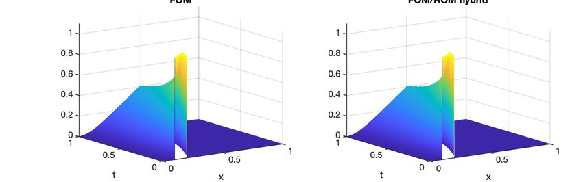
Figure 8: Time evolution plots of nonlinear circuit with the step input signal: (left) FOM, (right)
the hybrid model when w = 20 and tol = 10−4 .
We consider n̄ = 401 and the simulation time interval t ∈ [0, 10] seconds in this test. For the
time integration, we use semi-implicit method with Nt = 400 uniform time steps. In the hybrid
approach, we use the POD ROM, set the time window width w = 20 and the tolerance of output
error at each step to be 10−4 . The dual problem is solved once by a direct solver. The time
evolutions of the FOM and the hybrid model voltage values are shown in Figure 8 and the output
results are shown in Figure 9, respectively. It is seen that, compared with the FOM, the hybrid
approach obtains an accurate approximation. Time evolutions of the estimated error ∆k+1 and
“true” error are shown in Figure 10, which indicates that ∆k+1 provides a reliable indicator of
14the output approximation error at each time step. Note that, because the system input is zero in
the first 3 seconds, the estimated error is zero, which matches the real error in the time interval.
To make these errors visible in Figure 10 which has a log-scale y-axis, we set them to be the
floating-point relative accuracy (eps in Matlab notation).
10 -3
20
15
FOM/ROM Hybrid
FOM
10
5
0
0 1 2 3 4 5 6 7 8 9 10
Figure 9: Time evolution of the outputs from the FOM and the hybrid model.
10 -5
estimated error
true error
-10
10
10 -15
0 1 2 3 4 5 6 7 8 9 10
Figure 10: Estimated and true errors of the circuit problem during the simulation.
The total number of FOM runs during the hybrid model simulation is Nf = 40 times, which
includes 20 initial FOM runs at the beginning of the simulation. The hybrid model takes Pf =
10% of the total number of time steps. The CPU time for integrating the hybrid model is
th = 4.22 × 10⁻² seconds while the full order model simulation takes tf = 9.47 × 10⁻² seconds.
6 Conclusions
Multiple high-fidelity large-scale simulations are generally needed in building ROMs for complex
dynamical systems. These simulations provide snapshot data for which the reduced basis is
extracted and the solution manifold is approximated. In this paper, a FOM/ROM hybrid approach
is developed to accelerate such high-fidelity simulations. The development is based on an a
posteriori error estimation for the output approximation. By controlling the estimated error, the
method switches between the FOM and the ROM generated on the fly in a dynamical manner.
Numerical tests on the Burgers’ equation and a nonlinear circuit problem illustrates that the
hybrid approach is able to save the computational time while achieving a user-defined level of
accuracy. Our future work includes the hybrid MOR for systems with changing input signals, the
15extension of the error indicator to state approximations and the design of more efficient algorithms
for updating the ROM on the fly.
References
[1] M. M. A. Asif, M. I. Ahmad, P. Benner, L. Feng, and T. Stykel. Implicit higher-order
moment matching technique for model reduction of quadratic-bilinear systems. Journal of
the Franklin Institute, 358(3):2015–2038, 2021.
[2] F. Bai and Y. Wang. DEIM reduced order model constructed by hybrid snapshot simulation.
SN Applied Sciences, 2(12):1–25, 2020.
[3] F. Bai and Y. Wang. Reduced-order modeling based on hybrid snapshot simulation. Inter-
national Journal of Computational Methods, 18(01):2050029, 2021.
[4] K. Carlberg. Adaptive h-refinement for reduced-order models. International Journal for
Numerical Methods in Engineering, 102(5):1192–1210, 2015.
[5] S. Chellappa, L. Feng, and P. Benner. Adaptive basis construction and improved error
estimation for parametric nonlinear dynamical systems. International Journal for Numerical
Methods in Engineering, 121(23):5320–5349, 2020.
[6] F. Chen, J. S. Hesthaven, and X. Zhu. On the use of reduced basis methods to accelerate and
stabilize the parareal method. In Reduced Order Methods for modeling and computational
reduction, pages 187–214. Springer, 2014.
[7] V. Esfahanian and K. Ashrafi. Equation-free/Galerkin-free reduced-order modeling of the
shallow water equations based on proper orthogonal decomposition. Journal of fluids engi-
neering, 131(7), 2009.
[8] P. A. Etter and K. T. Carlberg. Online adaptive basis refinement and compression for
reduced-order models via vector-space sieving. Computer Methods in Applied Mechanics and
Engineering, 364:112931, 2020.
[9] C. Farhat, J. Cortial, C. Dastillung, and H. Bavestrello. Time-parallel implicit integrators for
the near-real-time prediction of linear structural dynamic responses. International journal
for numerical methods in engineering, 67(5):697–724, 2006.
[10] S. Fresca and A. Manzoni. POD-DL-ROM: enhancing deep learning-based reduced order
models for nonlinear parametrized PDEs by proper orthogonal decomposition. arXiv preprint
arXiv:2101.11845, 2021.
[11] C. Gu. QLMOR: A projection-based nonlinear model order reduction approach using
quadratic-linear representation of nonlinear systems. IEEE Trans. Comput. Aided Des. In-
tegr. Circuits. Syst., 30(9):1307–1320, 2011.
16[12] B. Haasdonk and M. Ohlberger. Reduced basis method for finite volume approximations
of parametrized linear evolution equations. ESAIM: Mathematical Modelling and Numerical
Analysis, 42(02):277–302, 2008.
[13] J. S. Hesthaven, C. Pagliantini, and N. Ripamonti. Rank-adaptive structure-preserving re-
duced basis methods for Hamiltonian systems. arXiv preprint arXiv:2007.13153, 2020.
[14] Y. Kim, Y. Choi, D. Widemann, and T. Zohdi. Efficient nonlinear manifold reduced order
model. arXiv preprint arXiv:2011.07727, 2020.
[15] K. Lee and K. Carlberg. Deep conservation: A latent-dynamics model for exact satisfaction
of physical conservation laws. arXiv preprint arXiv:1909.09754, 2019.
[16] K. Lee and K. T. Carlberg. Model reduction of dynamical systems on nonlinear manifolds
using deep convolutional autoencoders. Journal of Computational Physics, 404:108973, 2020.
[17] Y. Maday and O. Mula. An adaptive parareal algorithm. Journal of computational and
applied mathematics, 377:112915, 2020.
[18] R. Maulik, B. Lusch, and P. Balaprakash. Reduced-order modeling of advection-dominated
systems with recurrent neural networks and convolutional autoencoders. Physics of Fluids,
33(3):037106, 2021.
[19] B. Peherstorfer. Model reduction for transport-dominated problems via online adaptive bases
and adaptive sampling. SIAM Journal on Scientific Computing, 42(5):A2803–A2836, 2020.
[20] O. San and R. Maulik. Neural network closures for nonlinear model order reduction. Advances
in Computational Mathematics, 44(6):1717–1750, 2018.
[21] S. Sirisup, G. E. Karniadakis, D. Xiu, and I. G. Kevrekidis. Equation-free/Galerkin-free
POD-assisted computation of incompressible flows. Journal of Computational Physics,
207:568–587, 2005.
[22] Z. Wang, B. McBee, and T. Iliescu. Approximate partitioned method of snapshots for POD.
Journal of Computational and Applied Mathematics, 307:374–384, 2016.
[23] Y. Zhang, L. Feng, S. Li, and P. Benner. An efficient output error estimation for model
order reduction of parametrized evolution equations. SIAM Journal on Scientific Computing,
37(6):B910–B936, 2015.
17You can also read