Machine Learning and Neural Networks in Finance Machine Learning Models of Corporate Bond Relative Value - Risk Training
←
→
Page content transcription
If your browser does not render page correctly, please read the page content below

Machine Learning and Neural Networks in Finance
Machine Learning Models of Corporate Bond
Relative Value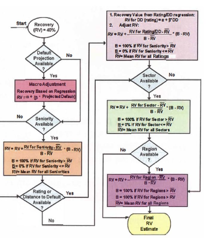
Corporate Bond Relative Value
The objective of this project is to improve upon our current method for beating corporate
bond indexes by adding variables and applying machine learning techniques.

 OVERALL GOAL: Outperform the cut-and-rotate method
 at beating corporate bond benchmarks
  ! In 2004, we developed a strategy that consistently outperforms global
    corporate bond indexes and have been testing it out-of-sample since
    then
  ! The strategy takes as input bonds' model-based expected default
    probabilities and recovery values in default along with credit spreads
    and applies rules for portfolio construction based on those inputs
  ! We wanted to use additional explanatory variables in a non-linear
    model to more accurately determine fair yield spreads and anticipate
    spread change/convergence
     ! Use neural networks to model non-linear relationship
  ! Using those network-based relative value numbers, test the
    performance of the new relative value numbers in our cut-and-rotate
    strategy
     ! Predict 1 month change in OAS directly

                                                                                            2
Benzschawel Scientific, LLC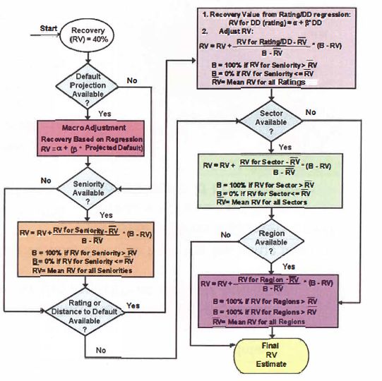
Bond Pricing – Yield Spreads to Treasuries
The yield spread to Treasuries is the market standard for quoting and evaluating the
relative riskiness among different corporate bonds and/or of different maturities.
                                                                        Yield Curves for US Treasuries and
● To isolate the price of credit risk, corporate                           for Single-A Corporate Bonds
  bonds are typically quoted on a yield                                               7

  spread-to-Treasury basis
  ⏤ The credit risk of a bond is the yield spread
                                                                                      6

                                                                                                          Credit Spread

    over the yield of a Treasury bond of similar

                                                                                (%)
                                                                                      5

                                                                        Yield (%)
                                                                       Yield
    maturity                                                                          4

  ⏤ To compute the present value of a bond with
                                                                                                      US Treasury Yields
                                                                                                      Corporate Bond Yields
                                                                                      3

    maturity, T:                                                                      2
                               é                 ù                                        0      5   10       15           20   25   30   35

                               ê2T -1   c        ú c + 100                                                Years    toMaturity
                                                                                                            Years to   Maturity

      for US Treasuries:   PV = å
                               ê          2      ú+ 2
                               ê t =1 æ r0.5t öt ú æ rT ö 2T
                               ê ç1 +         ÷ ú ç1 + ÷                                      Yield Spread by Agency Rating
                               ë      è   2   ø û è   2 ø Credit
                                                              Spread
                                é                     ù
                                ê2T -1    c           ú   c + 100
         for Corporates:   PV = ê å          2        ú+    2
                                ê t =1 æ r0.5t + s ö ú æ rT + s ö 2T
                                                    t

                                ê ç1 +             ÷ ú ç1 +     ÷
                                ë è          2 ø û è          2 ø
     Where PV is the price of bond with coupons (ct), rt
     is the term structure of US Treasury spot yields at
     0.5 year intervals, and s is the yield spread of the
     credit curve to US Treasuries. Spread is often                                            Yield spreads to Treasuries
     Basis Points where 1bp is 1/100 of 1%                                                     increase with maturity and
                                                                                               decreasing credit quality.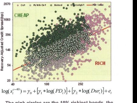
Calculating Bond Relative Value - Default Risk
    The success of our current "cut-and-rotate" strategy depends on having accurate estimates
    of bonds' expected probabilities of default and recovery values. We consider first our model
    for predicting bond defaults; Citi's Hybrid Probability of Default (HPD) model.

    ● We use the hybrid                                     Hybrid Probability of Default Model
      probability of default (HPD)
      model to estimate firms'
      probabilities of default
      ⎼ The model is called a "hybrid"
        because it combines a
        "Merton-type" structural model
        with statistical variables on
        firms' size, profitability and
        cash flow
      ⎼ This model is the best we know
        of commercial and industrial
        firms

    ● We use the Merton model framework because idiosyncratic risk
      in the equity market appears to lead the bond market
     ⎼ The equity market is larger, has more strategist coverage and is more
          liquid
8
      ⎼   It is cheapest to put on a view of credit in the equity market
                                      Benzschawel Scientific, LLC                                  4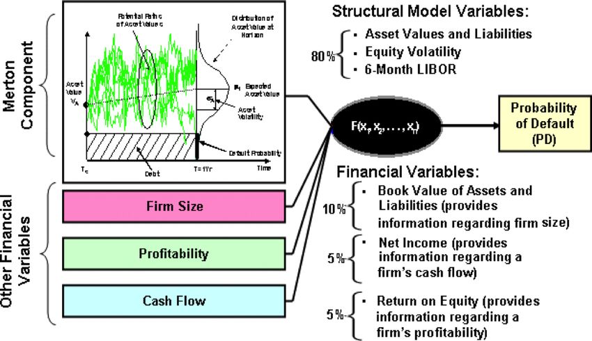
Bond Relative Value – Recovery Value
    Calculating
Expected              Bond Relative
          losses on corporate  bonds dependValue   - the
                                              on both Recovery      Value
                                                         likelihood of default and
recovery value in default. We use a decision-tree model of recovery value in default.
      Expected losses on corporate bonds depend on both likelihood of default and recovery value
●   The   decision-tree
      in default.              model
                  We currently use                       Model
                                   a decision tree model of      forvalue
                                                            recovery Recovery     Value in Default
                                                                          in default.
      • The decision-tree
    embeds                  model embeds of Model for Recovery Value in Default
               known determinants
        known determinants of recovery
    recovery
        value in value
                 default. in default
                           These are:
    ⎼ Credit cycle,
       ─ Credit       seniority,
                 cycle,              industry
                         seniority, industry
      sector, credit
          sector, creditquality
                          quality, and  geography
                                   and geography
       The tree begins by assigning a recovery rate of
       40% for all securities. If one has no other
       information, the tree will output 40%
       The first decision point is the adjustment for
       credit cycle dependency. The next step in the
       decision tree concerns seniority in the capital
       structure
       Following the hierarchy shown in the figure,
       we assign the firm's seniority to one of the
       following six categories

       The next adjustment in the model is for credit
       quality just prior to default. If nothing is input at
       this stage, the analysis advances to the sector
       adjustment stage
       The recovery value is then adjusted for
       industry sector

       The final adjustment is for geographical region
       as different regions have different bankruptcy
       regimes, legal procedures and precedents                Benzschawel Scientific, LLC
                                                                                                     5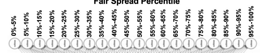
Corporate Bond Relative Value
We calculate bonds' relative values as the amount of credit spread for their default
probability, recovery value, and duration relative to the average of all bonds.
● We calculate bonds' relative                               Credit Spreads vs Log Default
  values by plotting their recovery-                         Probability and Log Duration
  adjusted spreads to Treasuries
  versus the logarithms of their one-
  year default probabilities and
  durations
   ⎼ Relative value is z-score vertical
     distance from the fair value line (the
     red line in the figure)
● The recovery-adjusted spread puts all
  bonds on a 40% recovery value basis
  and is calculated as:
                 (                  (45 6 789:;< ∗9;?@AB
   !"#$%& = − )*+,-"./   ∗ ln 1 −     ( 4+5#.C5+D +,-5

● Thus, our model for yield spreads to
  Treasuries for bond i is:                                   The pink circles are the 10% riskiest
                                                              bonds, the gray are 10% riches and
  log $%&'() = *)+ *+ ∗ -./ 01% + *2 ∗ -./ 134% + 5%          dark read are 10% cheapest
● The relative value measure adjusts for effects of duration and
  recovery value on spreads                                                                           6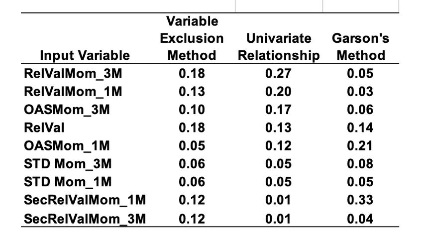
Predicting 1-Month OAS Changes
We decided to test if we could predict one-month changes in option-adjusted
credit spreads.
● We used our relative value measure and other variables as input to
  regression and neural network models to predict one-month changes
  in bond spreads to US Treasuries
! In addition to bonds’ relative values, we added the variables:
   ⎼   OAS Momentum (1M an 3M)
   ⎼   Relative Value Momentum (1M and 3M)
   ⎼   Spread-Times-Duration Momentum (1M and 3M)
   ⎼   Sector Relative Value Momentum (1M and 3M)

              Input Variables for 1-Month OAS Change Models

                             Benzschawel Scientific, LLC                      7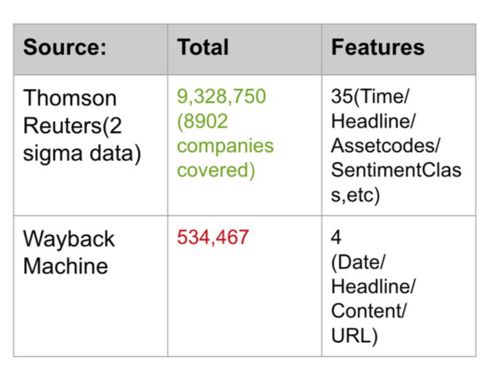
Input Variable Definitions
Because several of the variables are normalized with respect to changes in the
market, they are defined explicitly below.
● OAS Momentum N-Month:

● Relative Value Momentum N-Month:

● Spread Duration Momentum N-Month:

● Sector Relative Value Momentum N-Month:

                            Benzschawel Scientific, LLC                          8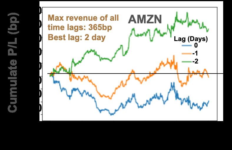
Network Architecture – The Output Layer
We chose a 20-bin output layer, scaled in units of 5% of the ranked population of
one-month spread changes and applied the Softmax function to normalize the
distribution.
● We rank all the                Output Layer (Relative Value Percentiles)
  relative value
  numbers in the
  training sample
  and convert them
  to percentiles as
  the dependent
  variable for each bond
● Then for each training case output, we apply the Softmax function
  which takes an un-normalized vector of density across the 20 bins and
  normalizes it into a probability distribution
● The standard (unit) Softmax function is given by the standard
  exponential function on each coordinate, divided by the sum of the
  exponential function applied to each coordinate
    — The sum of the exponential function acts as a normalizing constant, so
      the output coordinates sum to 1:

  Benzschawel Scientific, LLC                                                       9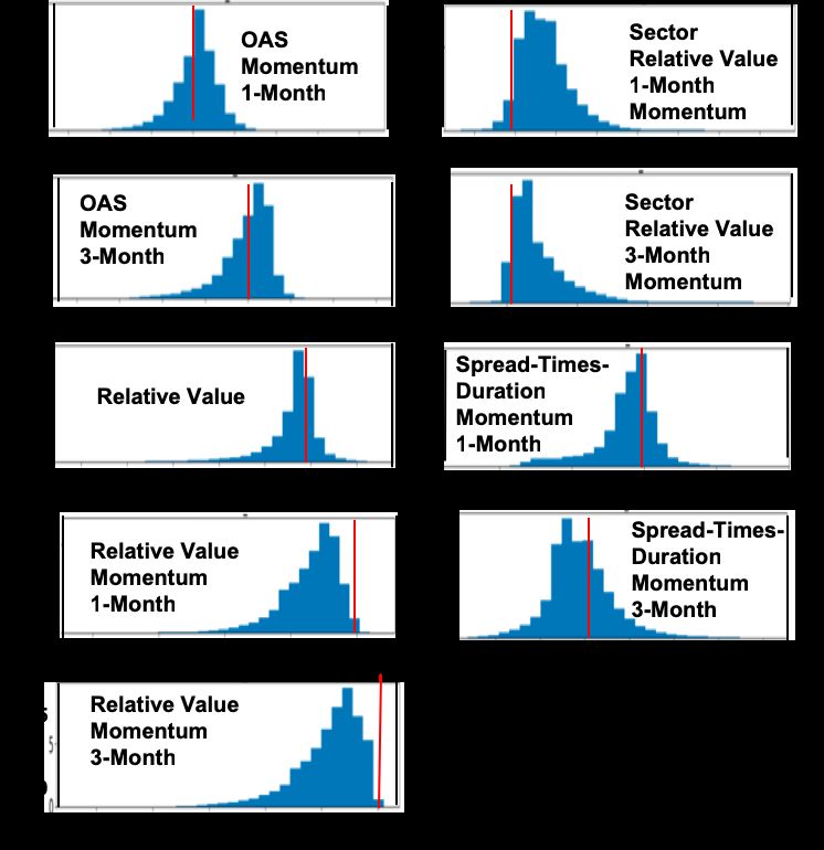
Choosing the Loss Function and Network Architecture
We chose the categorical cross entropy measure as the error function and
used it as a criterion for choosing the network architecture.
● We used categorical cross entropy as the error function

● The double sum is over the observations i, whose number is N, and
  the categories c, whose number is C
● The term          is the indicator function of the ith observation
  belonging to the cth category. The               is the model
  probability for the ith observation to belong to the cth category.
● The network outputs a vector of C probabilities, each giving the
  probability that the network input should be classified as belonging
  to the respective category
● We used the cross entropy error function as a measure for deciding
  on the structure of the network (see next slide)

                           Benzschawel Scientific, LLC                 10
Neural Network and Regression Model
We trained both a regression model and neural network model using the same
input variables using the same walk-forward procedure used previously.
● The regression model was an ordinary least squares regression
● The overall approach to the neural network architecture was similar to that
for the relative value network. That is,
— We used a standard Softmax function with 20 OAS bins as the output layer
of the network
— We used categorical cross entropy as the error function
● As before, to determine the
Categorical Cross Entropy Error vs
optimal neural network
Number of Nodes in Each Layer
architecture, we began with a
single node in a single hidden
layer, and add nodes and layers We kept the same
Error Magnitude
network structure for
until performance fails to all the years tested.
improve
— For example, the chart on the right
shows that a two-layer network is
preferable to a single layer
— We decided on a network with 2
hidden layers with 7 and 9 nodes,
respectively Number of Nodes
11
Benzschawel Scientific, LLCTraining the Network – The Walk Forward Procedure
We used a walk-forward procedure to train each network, each year adding the
data from the previous year.
● We used a ”walk forward” Illustration of Walk-Forward Network
procedure to train a series of Training Procedure
annual neural network models
2005 to Year X
— For example, the chart on the
right shows that the first
network model was trained
only on the data from 2005
— That model was used to
generate relative value
numbers for 2006
● Then data from 2006 were
added to the training
sample of 2005 and used to 05 06 07 08 09 10 11 12 13 14 15
train the model to test on
data from 2007
● This process continued until the final model in 2015 which trained on
data from 2005 through 2015 was used to generate predictions for 2016
— Thus, each successive annual model was trained on an increasing amount
of data
Benzschawel Scientific, LLC 120%-5%
5%-10%
of 10,000
10%-15%
Epochs with
15%-20%
The model was
trained for 5,000
20%-25%
Learning Batch Size
Bias - 25%-30%
Benzschawel Scientific, LLC
OAS Momentum 1M - 30%-35%
OAS Momentum 3M - 35%-40%
Relative Value - 40%-45%
Rel Val Momentum 1M - 45%-50%
Rel Val Momentum 3 M - 50%-55%
STD Momentum 1M - 55%-60%
STD Momentum 3M - 60%-65%
Sector Rel Val Momentum 1M - 65%-70%
OAS Spread Change Percentile
Sector Rel Val Momentum 1M - 70%-75%
75%-80%
80%-85%
85%-90%
ReLU
ReLU
Function
Function
90%-95%
95%-100%
to 1
Scaled in
Percentiles From 0
Input Variables are
Softmax Function
Corporate Bond 1 Month OAS Change Network
Layer 1 Layer 2
13
Input Layer Hidden Hidden Output LayerOne Month OAS Change Network Performance
Both the regression and neural net models of one-month OAS changes were
designed to select bonds on relative OAS change only.
● The 1-Month OAS change models predicted spreads directly, so did
not go through the cut-and-rotate paradigm.
● The OLS and neural net models had information ratios of 1.3 and 1.7,
respectively, mainly by reducing the volatility of returns
⎼ These are far superior to the 0.6 and 1.1 information ratios of the
benchmark and neural network cut-and-rotate strategies
Annual Returns and Summary Statistics from Relative Value and 1-Month OAS Models
OAS Relative Value Models 1 Month Change in OAS
Average Annual Benchmark Neural Network OLS Neural Network
Year Spread Change Cut Rotate CnR Cut Rotate CnR Cut Rotate CnR Cut Rotate CnR
2006 95 -5 4 30 38 -4 21 14 -5 -19 -22 -5 -16 -40
2007 196 111 -4 -15 -17 13 -18 4 11 -4 13 11 7 28
2008 676 477 56 -10 8 134 -92 62 134 180 291 134 63 252
2009 212 -403 -71 614 553 -188 386 147 -190 18 -126 -190 135 -39
2010 171 -18 -6 129 122 -4 79 73 -3 98 91 -3 88 96
2011 237 65 18 30 46 21 -2 20 19 76 96 19 83 124
2012 152 -85 5 121 137 -6 103 98 -8 94 93 -8 92 94
2013 131 -29 -11 27 20 -16 47 31 -15 83 62 -15 67 39
2014 126 12 7 72 93 15 81 104 15 57 71 15 73 82
2015 165 46 47 -15 39 63 -6 64 66 56 129 66 78 127
2016 136 -42 -64 116 35 -82 55 -27 -80 117 35 -80 107 22
Sum 2297 129 -19 1099 1074 -54 654 590 -56 756 733 -56 777 785
Mean 209 12 -2 100 98 -5 59 54 -5 69 67 -5 71 71
Std Dev 153 195 37 171 151 77 116 49 77 54 98 77 41 80
Ratio 0.0 0.6 0.6 -0.1 0.5 1.1 -0.1 1.3 0.7 -0.1 1.7 14
0.91-Month OAS Change Model Performance (cont.)
We also analyzed models’ performance using monthly returns by relative value
decile. 1M Change in OAS - Neural Net Model
1M Change in OAS - OLS Model
120
1M Change - Neural Network
Neural Net Model
● We analyzed 10
1M Change - OLS Model Annual Annual Info
OLS Model
Cumulative Uncompounded Return (% )
100 Annual Annual Info
10 Decile Mean StdDev Ratio
Cumulative Uncompounded Return (% )
Decile Mean StdDev Ratio 1 10.09 6.05 1.67
9 100
1 8.93 6.33 1.41 2 8.57 6.25 1.37 9
monthly returns 80
2
3
4
8.54
7.86
7.42
6.13
6.57
6.53
1.39
1.20
1.14
8
7
6 80
3
4
5
7.84
7.52
6.82
6.84
6.42
6.03
1.14
1.17
1.13
8
7
5 7.07 6.80 1.04 Idx 6.23 5.73 1.09
6
by decile for the 60
Index
6
7
6.23
5.91
5.62
5.73
6.27
5.49
1.09
0.94
1.02
5
4 60
6
7
8
5.94
5.43
4.11
5.56
5.60
5.84
1.07
0.97
0.70
5
4
3 9 3.48 5.61 0.62
OLS and neural
8 5.67 5.37 1.06
9 3.30 5.49 0.60 10 2.47 5.31 0.47
10 1.95 5.34 0.36 3
40 40
2
network 1-month 20
2
1 20
1
change models 0
0
● Both models -20
-20
2006 2007 2008 2009 2010 2011 2012 2013 2014 2015 2016 2017
perform well at 2006 2007 2008 2009 2010 2011 2012 2013 2014 2015 2016 2017
ranking absolute 1M Change - OLS Model
1M Change - Neural Network
Annual Annual Info
and risk adjusted Annual Annual Info
Decile Mean StdDev Ratio
Decile Mean StdDev Ratio
returns by decile 1
10 8.93 6.33 1.41
1
10 10.09 6.05 1.67
29 8.57 6.25 1.37
29 8.54 6.13 1.39
● Returns from 38 7.86 6.57 1.20
38 7.84 6.84 1.14
decile 10 versus 47 7.42 6.53 1.14 47 7.52 6.42 1.17
56 7.07 6.80 1.04 56 6.82 6.03 1.13
decile 1 are 50bp Index 6.23 5.73 1.09
Index 6.23 5.73 1.09
per annum 65 5.91 6.27 0.94 65 5.94 5.56 1.07
74 5.43 5.60 0.97
greater for the 74 5.62 5.49 1.02
83 4.11 5.84 0.70
83 5.67 5.37 1.06
neural network 92 3.30 5.49 0.60 92 3.48 5.61 0.62
model 1
10 1.95 5.34 0.36 1
10 2.47 5.31 0.47
15
Benzschawel Scientific, LLC1-Month OAS Change Model Performance (cont.)
We analyzed profitability from each model of going long the bonds in decile 10
and short the bonds in decile 1
● Both OLS and Neural Net models perform well in decile 10 versus decile 1
long/short trades
⎼ The OLS model has 74% profitable months with an average return of 56bp
(6.72% per annum) and an information ratio of 1.4
⎼ The neural network was profitable 77% of months with an average return of
63bp (7.56% per annum) and an information ratio of 1.7
● The Neural Network model performs best
Monthly Returns and Summary Statistics from 1-Month OAS Models
8 8
Monthly Return (Long - Short)
Monthly Return (Long - Short)
Profitable Months = 77%
Profitable Months = 74% Average Monthly Retrun = 63bp
6 6
Average Monthly Retrun = 58bp Annual Sharpe Ratio -= 1.68
Annual Sharpe Ratio -= 1.43
4 % 4
%
2 2
0 0
-2 OLS Model -2 Neural Net Model
-4 -4
2006 2007 2008 2009 2010 2011 2012 2013 2014 2015 2016 2017 2006 2007 2008 2009 2010 2011 2012 2013 2014 2015 2016 2017
160 Benzschawel Scientific, LLC 16
rn
901-Month OAS Change Model Performance (cont.)
We analyzed cumulative profitability from each model of going long the bonds in
decile 10 and short the bonds in decile 1
● We analyzed cumulative uncompounded returns from the OLS and Neural
Network Models
● Models perform similarly as regards profitable years and drawdowns, but
the Neural Network had higher overall returns
⎼ Both are profitable 10 of 11 years and drawdowns are -1.9% and -2.4%, but the
neural network has higher absolute returns
● Both models have steady returns after the credit crisis of 2008-2009
⎼ Recall the because of the “walk-forward” procedure, the samples for the
models increase as time goes on
2006 2007 2008 2009 2010 2011 2012 2013 2014 2015 2016 2017
Monthly Returns and Summary Statistics from 1-Month OAS Models
90 90
80 Profitable Years = 10 of 11
Cumulative Uncompounded
80 Profitable Years = 10 of 11
Cumulative Uncompounded
Maximum Drawdown = -1.9% in Feb 2007 70 Maximum Drawdown = -2.4% in Mar 2007
70
60
Return (%) 60
50
Return (%)
50
40 40
30 30
20 20
3
10 OLS Model 10
Neural Net Model
0 0
-10 -10
2006 2007 2008 2009 2010 2011 2012 2013 2014 2015 2016 2017 2006 2007 2008 2009 2010 2011 2012 2013 2014 2015 2016 2017
Benzschawel Scientific, LLC
17Analysis of Variable Contributions – 1M OAS Change
For the 1-month OAS change network, there is greater dispersion of variable
importance rankings among analysis methods.
● Relative value Importance of Variables in OAS Change
momentum is Neural Network
important in variable
exclusion and
univariate analyses
⎼ However, they are
relatively
unimportant using
Garson’s method
⎼ Garson’s method
ranks relative value
and 1-month OAS
momentum as most
important
● Sector relative value momentum at 1M and 3M is important in
variable exclusion and Garson’s method, but have only a weak
univariate relationship to OAS changes
18
Benzschawel Scientific, LLCVariable Contributions - Derivative Analysis
The analysis of derivatives confirms the importance of relative value momentum
in the neural network model, but relative value and STD momentum are important
● As for the exclusion Summary Statistics from Derivative Analysis
and univariate Std
Input Variable Mean Deviation Skew Kurtosis
methods, the derivative
OASMom_1M 0.03 0.05 0.71 3.58
method assigns
OASMom_3M 0.00 0.05 -0.75 3.91
greatest importance to SecRelValMom_1M 0.02 0.02 1.27 3.52
1-month relative value SecRelValMom_3M 0.02 0.05 0.32 7.59
momentum RelVal -0.09 0.07 -1.58 5.24
STD Mom_1M -0.07 0.15 -0.72 3.49
⎼ 3-Month relative
STD Mom_3M 0.01 0.12 1.86 6.87
value momentum is RelValMom_3M -0.06 0.04 -1.71 5.26
also important RelValMom_1M -0.09 0.06 -1.69 5.22
● Consistent with
Garson’s method, relative value is tied with relative value momentum
as the third most important variable
● Average values of sector relative value momentum and OAS
momentum indicate little directional bias in the effects of those
variables.
19
Benzschawel Scientific, LLCVariable Contributions – Distribution of Derivatives
The derivative method provides information regarding the strength of each
variable, but the direction and consistency of its contribution.
● The distributions of Distribution of Derivatives for Input Variables
derivatives show that
variables whose mean
derivatives are close to
zero can have large
influences on network
responses
Probability Density (Sum to 100)
⎼ For example, OAS
momentum (1 and 3
month) derivatives
have broad
influences, but in
both directions
● Increases in relative
value and relative value
momentum consistently
lead the model to
predict tighter spreads
Benzschawel Scientific, LLC Value of Derivative 20Machine Learning and Neural Networks in Finance
Predicting Market Moves from News
HeadlinesProject Objectives The objective of this project was to generate sentiment scores from news headlines and use those scores to predict credit spread moves. ● In this project, we focused on using Natural Language Processing (NLP) techniques to build trading strategies for 1-day horizons for the corporate bond market using news headlines. ● Using data scraped from multiple financial sources, we employ machine learning approaches of varying complexities ● We find that pure sentiment prediction does not require models of very high complexity, but the link between sentiments and predictability of returns is not straight- forward ● We also find that approaches using the latest advances in NLP are better suited to predict future returns in credit indices, by using news headlines directly as inputs, instead of news headline sentiments
Introduction and Background
The objective of this project was to generate sentiment scores from news
headlines and use those scores to predict credit spread moves.

Natural Language Processing (NLP)
● Natural language processing (NLP) is a branch of artificial
  intelligence that is being used more and more for both
  business and financial applications
  − Financial institutions, on both the buy- and sell-sides, are adopting the
    technology for tasks like robo-advisories, credit checks, employee
    surveillance, and investment strategies
  − Financial literature on NLP has focused on metrics related to corporate
    governance, competitive dynamics, management quality, etc. that would
    be useful for longer-term investment signals in equity markets

● Traditional approaches have generally focused on
  conventional NLP methods like bag of words, TF-IDF scores to
  rank firms based on the frequency of occurrences of pre-
  defined “relevant” words in the firms’ 10-Ks, analyst reports,
  earnings call transcripts or news
   − There has also been progress in parsing through high-frequency
     information sources like news, employing the information gleaned in
     high frequency trading
Bag of Words
● Bag of Words (BoW) is an algorithm that counts how many
times a word appears in a document
− Those word counts allow us to compare documents and gauge their
similarities for applications like search and document classification
● BoW lists words paired with their word counts per document
− In the table where the words and documents that effectively become
vectors are stored, each row is a word, each column is a document, and
each cell is a word count
− Each of the documents in the corpus
is represented by columns of equal
length
− Those are wordcount vectors, an
output stripped of context
● Before they’re fed to the neural network, each vector of wordcounts
is normalized such that all elements of the vector add up to one
− Thus, the frequency of each word is effectively converted to represent the
probabilities of those words’ occurrence in the document
− Probabilities that surpass certain levels will activate nodes in the network
and influence the document’s classificationTerm Frequency-Inverse Document Frequency
(TF-IDF)
Term-frequency-inverse document frequency (TF-IDF) is another way to
judge the topic of an article by the words it contains.
● With TF-IDF, words are given weight – TF-IDF measures relevance,
not frequency
− Wordcounts are replaced with TF-IDF scores across the whole dataset
● TF-IDF measures the number of times that words appear in a given
document (that’s “term frequency”).
− Because words such as “and” or “the” appear frequently in all documents,
those must be discounted
− That’s the inverse-document frequency part. The more documents a word
appears in, the less valuable that word is as a signal to differentiate any
given document
− That’s intended to leave only the frequent and distinctive words as markers.
Each word’s TF-IDF relevance is a normalized data format that also adds up
to one.
− Those marker words are then fed to the neural net as features in order to
determine the topic covered by the document that contains themIntroduction and Background (cont.)
One common problem is that old approaches (like bag of words) lead to
highly sparse predictor matrices.
● A standard way of dealing with the sparse matrix problem is creating
vector representations for each word, called the “word2vec”
algorithm (Mikolov, et al., 2013)
− Word2vec is a step towards transfer learning - for instance, Google has
trained a freely-downloadable word2vec model outputting word
representations using over a 100 billion words from a Google news dataset
● There are some issues with using off-the-shelf word2vec models
− One problem is that the data on which the model is trained is generic - it
encompasses non-financial data, leading to meanings which might not
make much sense in our context
− For instance, the closest words to “bull” in the Google word2vec model
would be other animals like “cow” and “dog”, whereas we want to see
similar words like “bear”, “rally” and so on
● Li and Shah (2017) used finance-relevant text data from micro-
blogging sites (StockTwits, Twitter) to train their word2vec models
− They created sentiment-specific embeddings so as to be able to predict
text sentiment of any given text for any firmIntroduction and Background (cont.)
● Moore and Rayson (2017) used news headlines to train a
word2vec model*
− Moore et al. try to predict sentiments in headlines concluding that
deep learning approaches like Bidirectional Long-Short Term Models
(BiLSTM) beat simpler approaches like Support vector Regressions
(SVR) by 4-6%
● Schumaker and Chen (2007) take a linguistic approach to
predicting intraday stock movements based on financial
news
− They extract specific phrases from all documents split by sector,
leading to a less sparse predictor set than a simple Bag of Words
approach
− They conclude that firm- / sector-specific training for their models
leads to better performance
● Recent work by Velay and Daniel (2018) used top 25 news
headlines to predict the end-of-day value of the DJIA index
− They tried both statistical and deep learning models, but find that
deep learning algorithms had difficulty figuring out the link between
the headlines and the index trend
* They have kindly open-sourced their model which we use for one of our approachesIntroduction and Background – Our Approach
In this project, we incorporate lessons from the above cited literature
(among others) as we attempt to use sentiment data to predict corporate
bond prices.
● Most previous approaches approaches have focused either
on pure sentiment prediction, or on its effects in liquid
markets like equities, with little attention being given to
credit markets.
● This study explores different approaches to predicting
corporate bond price moves over a 1-day horizon, using a
self-sourced dataset of news headlines
● We focus on both single-name credits as well as the
investment grade and high yield credit index ETFs
− These different levels of aggregations carry their own benefits and
challenges.
− One obvious benefit for single-name credits is the better one-to-one
correspondence between a news item and the firm
− However, there are fewer headlines for individual firms than the
market and trading single-name credits involves relatively high
transaction costsThe Data
Headline data were collected from major finance news sources such as Wall
Street Journal, Yahoo Finance, Washington Post and PR News
● Data were collected
using the Wayback
machine
− The Wayback Machine
was launched in 2001 to
address the problem of
website content
vanishing whenever it
gets changed or shut
down
− The service enables
users to see archived
versions of web pages
across time, which the
archive calls a "three
dimensional index".
− Kahle and Gilliat created
the Wayback machine
hoping to archive the
entire Internet and
provide "universal
access to all knowledge."Data - Sources
In addition to the data from the Wayback machine, we were able to find
sentiment scores from the Thomson-Reuters 2 Sigma data.
● Wayback Machine Data (Crawl Data Source Properties
Data)
− The raw html files contain the date,
headline, content, and link for each
news item
− There is no sentiment data
associated with the news items
− Although there are headlines, there
is typically very little additional news
● 2 Sigma Data
− The participants were given access
to organized and comprehensive finance data provided by 2 sigma (from
2007-01-01 to 2018-07-31, total 9 million rows).
− This dataset contains information at both article level and asset level and
includes article details, sentiment and other commentary
− The sentiment class in the news data indicates the predominant sentiment
class for this news item regarding to the specific asset
− Sentiment for each item is divided into three classes: Negative, Neural and
Positive, then selected the class with the highest probabilityWayback Data by News Source
We extracted a total of over 500,000 news headlines from the Wayback
machine beginning in 2000.
Number
● The aggregated level data was obtained by crawling the web
● Duplicate headlines were dropped from the dataset
● Over half of the data comes from the Wall Street Journal
(WSJ)Company Coverage
In addition to the data from the Wayback machine, we were able to find
sentiment scores from the Thomson-Reuters 2 Sigma data.
● We chose two corporate bond index: LQD (investment-grade)
and HYG (high yield) as our analysis targets
− The charts below show the number of news stories for each company
covered in the 2-sigma data
Netflix Inc
Spirit Communications
Tesla
First Chrysler Autos
Continental Resources
Tenet Healthcare
Community Health Systems
Sirius XM Radio
Western Digital Corp
International Game Tech
HCA Holdings
Investment United Rentals High
Scientific Games
Grade Clear Channel Holdings
Yield
First Data Corp
Zayo Colocation
0
600
200
400
800
1000
1200Predicting Returns from Individual Firms
In our first set of studies we summed the sentiment scores from the 2 sigma
data on individual firms and used it to go long or short their bonds.
● Trading strategy for Individual firms from sentiment data
− For each target company, aggregate all the news before 4 pm on each
trading day and sum their daily sentiment scores
− Go long their bonds if the sum of daily scores is positive; go short if
negative; and do nothing if zero
− Trade with that day’s closing price and close position on the next trading
day’s closing price
− Test on different Daily Sentiment Scores for Amazon
time lag of the
signals
AMZN
10
Daily Sentiment Score
● An example of the
summed daily
0
sentiment scores
for Amazon -10
appears on the
right -20
77 Trading Days
9/2012 10/2012 11/2012 12/2012 1/2012Sentiment Strategy for Individual Firms We calculate the daily P/L of our long/short trades based on sentiment data by looking at the change in spread on the bond over the period in question. ● For a long position in a given bond, we calculate the daily P/L as: which is the change is spread times the duration of the bond. ● For a short position in a given bond, the P/L is the negative of the long position P/L above ● To eliminate the effect of changes in market spreads, we hedge the single name companies with the LQD index ● That is, we take the P/L of a single firm and subtract the appropriate P&L of the index for each trading day ● Use the adjusted duration and spread change of LQD index to get the daily P/L of the firm in question
Some Examples of Results for Individual Firms
We provide some examples of cumulative uncompounded returns from
bonds of individual firms based on sentiment long/short trades (ignore
transactions costs)
                     800
                               CVS
 Cumulate P/L (bp)

                     600
                     400
                     200
                      0
                -200
                -400
                           0     200    400   600     800   1000
                                       Trading Days

                                                                   ● The performance differences
                                                                     across different time lags vary,
                                                                     which may indicate the limited
  35                                                                 power of the strategy
Firm Level Sentiment Prediction We will not have access to 2 Sigma data going forward, we decided to build a model to mimic the 2 Sigma sentiment scores and use the to predict market moves. ● We will not have access to the 2 Sigma data going forward ● Need to “back-calculate” firm-level sentiment model from given information so as to be useful in trading ● Disadvantages of neural nets for sentiment prediction − Too complex − ~100k parameters − Computationally difficult to train ● Past approaches have shown benefits of simpler models like Naive Bayes in sentiment classification, after appropriate text clean-up ● We decided to build a boosted tree model trained on the 2 Sigma data to generate sentiment scores ● We then would use those sentiment scores to try to predict market moves for individual firms.
You can also read