ISPD: an iconic-based modeling simulator for distributed grids
←
→
Page content transcription
If your browser does not render page correctly, please read the page content below
iSPD: an iconic-based modeling simulator for distributed grids
                  Aleardo Manacero, Renata S. Lobato, Paulo H.M.A. Oliveira, Marco A.B.A. Garcia,
                          Aldo I. Guerra, Victor Aoqui, Denison Menezes, Diogo T. da Silva
                                          Univ. Estadual Paulista - UNESP
                                       Computer Science and Statistics Dept.
                                          (aleardo,renata)@ibilce.unesp.br

Keywords: iconic modeling, grid simulation, distributed           [4] and Gridsim [3], being strongly dependent of scripting
systems                                                           languages.
                                                                     In this paper we describe an iconic based simulator, iSPD
Abstract                                                          (iconic Simulator of Parallel and Distributed Systems), which
Simulation of large and complex systems, such as computing        allows the creation of grid models through a graphical envi-
grids, is a difficult task. Current simulators, despite provid-   ronment. The simulator transforms the graphical model into a
ing accurate results, are significantly hard to use. They usu-    queue system, which is executed to provide performance data
ally demand a strong knowledge of programming, what is            for the user. The whole process can be performed very intu-
not a standard pattern in today’s users of grids and high per-    itively, starting from the iconic model of the grid that needs
formance computing. The need for computer expertise pre-          to be simulated, including its resources and tasks that must be
vents these users from simulating how the environment will        executed.
respond to their applications, what may imply in large loss of       In the following pages we firstly contextualize iSPD among
efficiency, wasting precious computational resources. In this     the other grid simulators available, then describe its specifica-
paper we introduce iSPD, iconic Simulator of Parallel and         tion and design. Results from its use are also provided, along-
Distributed Systems, which is a simulator where grid mod-         side the conclusions drawn from these tests.
els are produced through an iconic interface. We describe the
simulator and its intermediate model languages. Results pre-      2.   RELATED WORK
sented here provide an insight in its easy-of-use and accu-
                                                                     Grid simulators are in use for several years now. Some dif-
racy.
                                                                  ferent simulators have been proposed, although only a few
                                                                  are regularly used. During this section a brief description of
1.   INTRODUCTION                                                 them is provided. A greater attention will be provided to the
   The use of high performance computing is growing re-           mainstream simulators, Simgrid and Gridsim, since they are
markably in this century. It is not restricted to high-end sci-   well maintained and developed.
entific applications anymore. This growth has been enabled
by the introduction of less expensive systems associated with     Simgrid [5] is the first simulator proposed and still one of
the use of resource sharing systems, such as computer grids.      the most used. Its initial goal was the evaluation of centralized
As a result of the improved demand a large amount of HPC          scheduling policies for heterogeneous and distributed com-
users that are neither computer experts nor have a large com-     putational environments. New versions of Simgrid have been
puter support team to help with system analysis has appeared.     released continually, although it still lacks an easy-to-use in-
These new users create a new demand to HPC developers,            terface to create models. One of its strenghts is the capability
which is the creation of easy-to-use tools for system’s eval-     to model background traffic and computation, which is not
uation, since they need to grasp the best performance of an       present in most simulators. Models are configured by XML
environment that they do not fully understand.                    and C files, which is not easy for non-expert users. Currently
   Among the tools for system’s evaluation there are a wide       there is a GUI, Grid Matrix [12], that allows for an easy con-
range of simulators. Simulation is considered an important        trol of the simulation process, besides the schedulers continue
approach for performance evaluation since it can provide          to be provided through their actual codification in C.
modeling flexibility with reasonable accuracy. It is also rel-
atively cheaper than actual benchmarking and can be used          GridSim [3] is another largely used simulator, currently in
in any stage of a system development. The major drawback          its version 5.0. It allows for modeling of different classes of
with simulation is that most of simulators demand the knowl-      environments, including schedulers and machines. It is based
edge of specific programming languages, either simulation or      in the SimJava simulation engine. It is quite flexible and has
conventional languages. In the case of grid simulators this is    an interface that makes easier to model some types of com-
totally true, with the most influential tools, namely Simgrid     puting grids. It is more portable than other simulators since is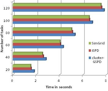
Java-based. Models are built through a Java program, using
pre-build classes for tasks and other components.
System model
GangSim [6] was developed to evaluate scheduling poli- ICONIC
cies in grid environments. It allows the analysis of interac- Iconic Model
INTERFACE
tions between local and global schedulers. This feature is very Results
interesting and it is under development in iSPD. Gangsim, as
the other simulators, does not enable an easy modeling inter- Simulatable Model
face, demanding the writing of scripts in an internal language. SIMULATOR
OptorSim [2] was initially developed to evaluate dynamic
replication algorithms used to optimize data location over the MODEL
grid. Optorsim has been used in this field, which is a ma- INTERPRETER Worlkload
jor difference when compared to the usual application of grid Database
simulators in scheduling analysis. Compared with iSPD it
does not have a simple interface to model grids while iSPD is External Models
not currently capable to manage data replication. Figure 1. iSPD Basic Structure
BeoSim [8, 9] is a discrete event simulator aimed to com-
puter grids assembled as Beowulf clusters, interconnected Grids can be simulated through some basic components,
through a dedicated network. It enables the evaluation of such as clusters, communication links, and individual hosts.
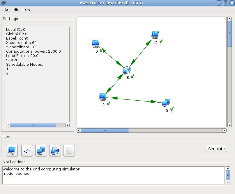
smaller grids under different workloads and scheduling poli- A basic model can be depicted in Figure 2, where the model
cies. contains three individual nodes (nodes 0, 1 and 2), a clus-
ter (node 3), a pointo-to-point communication link (between
GSSIM (Grid Scheduling Simulator) [7, 10] was built
nodes 1 and 3) plus internet connections (internet cloud is
over GridSim aiming to solve the problems with workload
node 8). From this figure it is also possible to identify the
generation and scheduling levels present in other simulators.
components in the interface. The main component is the
These simulators have been used mostly to evaluate drawing sector, where the user actually draws the model to
scheduling policies. In order to perform such evaluation, it is be simulated. On its side there is an information display, the
necessary to model the grid (hosts and networks), the work- “Settings” window, which shows the parameters of a selected
load, and the scheduling policies themselves. These tasks are icon (node 0 in that case). Just below these windows there
not easy to perform in the simulators just described. iSPD, are the icons menu and the “Simulate” button. Finally there
however, makes all these tasks easier to be performed while is the “Notifications” window, where a log of the session is
providing comparable accuracy. Hosts and their connections registered.
are easily modeled by an iconic interface, while the schedul- Once the model is entered to the system, the interface gen-
ing policies are parameters provided to specific components erates a text file containing its description, using a block-
and may also be modeled through a simple interface. based iconic description language. This language describes
a grid through a set of individual description blocks using a
specific grammar for this. Figure 3 shows the file created for
3. THE iSPD the model drawn in Figure 2. This file is then interpreted by
The design of iSPD is structured in three basic modules: the model converter, leading to a second text file containing
the graphical interface, the language interpreter/decoder and the grid described as a queue model using a queueing descrip-
the simulation engine. Besides these modules, some addi- tion language 4.
tional interfaces are present, mostly concerned with import- Although the use of two different languages may seem
ing/exporting models and metrics collection. The interaction clumsy, it saves a lot of effort when dealing with imported
between modules can be seen in Figure 1. In that Figure one models. Using this approach it is possible to restrict the con-
sees that the user inputs the model through an iconic model, version to/from other simulators to the iconic language, en-
which is translated to a simulatable model, receiving the re- abling the user to easily recover models built for those simula-
sults from its simulation. The simulation can make use of a tors to the iSPD iconic interface. Using a separate language to
workload database or a random workload. There is also the describe the simulation constraints and model also avoids the
possibility to convert external models to an iconic model or need for queue-oriented parameters or objects in the iconic
vice versa1 . interface. Figure 4 shows part of the queueing model for the
1 Currently it is possible to convert Simgrid models to iSPD models given example, where some lines were omitted for the sakeMODEL
TASK
RANDOM 11 28 55 0.98
11 16 22 1.0
0 2 30
END_TASK
SERVICE_CENTERS
CS_0 cs_icon1 1 1 QUEUES q_icon1 SERVERS
serv_icon1 0 1200.000 30.000 MASTER RoundRobin LMAQ cs_icon3
CS_2 cs_lan13 1 1 QUEUES q_lan13 SERVERS
serv_lan13 1 10000.000 10.000 0.400000
.
.
.
CS_1 cs_icon3 2 8 RoundRobin QUEUES q_0_icon3 q_1_icon3 SERVERS
serv_icon3 0 20000.000 10000.000 0.400000
CS_2 cs_lan10 1 1 QUEUES q_lan10 SERVERS
serv_lan10 1 10000.000 10.000 0.400000
END_SERVICE_CENTERS
CONNECTIONS
cs_icon111 cs_lan13
.
.
.
cs_icon2 cs_lan10
cs_lan10 cs_icon111
Figure 2. iSPD Basic Structure END_CONNECTIONS
END_MODEL
HOST icon1 1200.000 30.000 MASTER RoundRobin LMAQ icon3
HOST icon2 2000.000 30.000 SLAVE Figure 4. An example of iSPD’s queueing description lan-
HOST icon0 2000.000 20.000 SLAVE guage
CLUSTER icon3 8 20000.000 10000.000 0.400000 RoundRobin
INET icon111 20.000 1.000000 40.000
LINK lan7 10000.000 0.400000 10.000 CONNECTS icon3 icon1
LINK lan10 10000.000 0.400000 10.000 CONNECTS icon2 icon111 • User’s satisfaction, as a measure of fairness in user’s at-
LINK lan5 10000.000 0.400000 10.000 CONNECTS icon1 icon3
LINK icon14 10000.000 0.400000 10.000 CONNECTS icon1 icon111 tention; and
LINK lan12 10000.000 0.400000 10.000 CONNECTS icon111 icon0
LINK lan11 10000.000 0.400000 10.000 CONNECTS icon111 icon1 • Average waiting times, as a measure of contention for
LINK lan13 10000.000 0.400000 10.000 CONNECTS icon111 icon2
LINK lan9 10000.000 0.400000 10.000 CONNECTS icon0 icon111 resources.
LOAD RANDOM
11 28 55 0.98
11 16 22 1.0 In order to correctly model a grid environment through
0 2 30 a queueing network it was necessary to map each resource
type to a network configuration. This resulted in modeling
communication links and single hosts as 1-queue-1-server
Figure 3. An example of iSPD’s iconic description language networks, computer clusters as 1-queue-N-servers, and the
whole grid as N-queues-N-servers. In fact, a grid can be seen
of simplicity. as a recursive assembly of clusters, single nodes and commu-
The process continues with the simulation engine initially nication links.
converting the simulatable model to a queueing network. Although the user may configure the probability distribu-
Once the network is created, iSPD starts the model simula- tion functions used by the service centers in the queueing
tion using scheduling policies provided as grid parameters. network, there are few distributions that must be present as
Results from the simulation are then aggregated in order to defaults. Therefore, iSPD offers random generators for the
provide a series of performance metrics for the user. The file Poisson, exponential and two-stage uniform functions. The
containing the results is very large and will not be shown here. choice for these functions is based on previous results pro-
It basically contains the whole simulation history, from which vided by Lublin and Feitelson [11], showing that they make
performance parameters are extracted. The performance met- good models for distributed systems.
rics currently provided by iSPD include:
3.1. Iconic and Queueing languages
• Average turnaround times, as the average time spent to
complete each task; The core of iSPD is the use of two languages to represent
the iconic, graphical in nature, model, and the simulatable
• System’s efficiency, as a measure of system demand and model. The grammars for these languages are reasonably sim-
occupation; ple, generated using context-free grammars that include allneeded objects to create those models. Here we provide only manding information about processing speed and occupation
the main parts of the grammars that generate the models. for example. SC1 is mapped to clusters, demanding informa-
The grammar of the iconic modeling language is context- tion about local bandwidth, processing speed, occupation and
free, with a reasonably small amount of symbols. The re- scheduling policy. SC2 is mapped to communication links
served words in this language include “HOST”, “CLUS- and SC3 to the internet cloud.
TER”, “LINK”, “INET”, “MASTER”, “SLAVE”, and few
other internally defined terms for input parameters. The start- ::= SERVICE_CENTERS END_SERVICE_CENTERS
ing token for a model specification is . It leads to a ::= |
::= | | |
list of the available icons from the user interface. The rules ::= SC_0 QUEUES SERVERS
in Figure 5 describe the model global specification and the ::= SC_1 QUEUES
SERVERS
HOST grammar rules. The grammar rules for the remaining ::= SC_2 QUEUES SERVERS
components of a model, which are similar to the rules for ::= SC_3 QUEUES SERVERS
::=
HOST, will be ommited here. ::=
::=
::=
::=
::= {}+
::= | | | |
::= HOST Figure 7. Description of service centers invf the queue de-
::= MASTER HOST_LIST | SLAVE scription language grammar
::=
::=
::=
::= RR | WORKQUEUE | FPLTF
::= {}+ 3.2. Simulation engine
Figure 5. Section of the iconic description language gram- The simulation engine reads the system’s model, after its
mar conversion from the iconic to the queueing model and sim-
ulates it through an event-based process. It is composed by
The first three lines in figure 5 define the icons that are two modules: one that manages the service centers, includ-
present in the modeling interface. The fourth line is the start- ing queues and their respective servers, and other that man-
ing point for the definition of a single host in the model. As it ages the scheduling policies used by each server. The differ-
can be seen, the icon for a host is described by rules defining ent events managed by the simulation engine are:
the node type (master or slave), processing capacity (comput-
ing power) in MFlops, and load average (percentage). If the • Task arrival: when a specific task is added to a server’s
node is a master it also defines the scheduling algorithm and queue;
the list of slaves attached to it. • Task service: when a task is served by the server;
Using the same approach, the grammar of the queue mod-
eling language is also context-free and reasonably simple. • Task delivery: when a task is removed from a service
Figure 6 shows the top levels of the grammar for the queue center and, eventually, creates a new Task arrival in an-
modeling language. Line 1 shows the starting symbol for this other center.
grammar (), while the remaining lines de-
scribe the starting ramifications for the rules defining service Figure 8 shows how the simulator works. It follows the
centers and the connections between them. Event Scheduling/Time Advance [1] model, managing the fu-
ture events (FE) list through correct insertions and removals,
::= MODEL END_MODEL
and adjusting the simulated time. When no more events are
::= | present in the list, the engine produces all relevant metrics
::= | |
::= CONNECTIONS END_ CONNECTIONS
that may have interest for the grid evaluation.
::= | Each element from the grid model is mapped to specific
::= SERVICE_CENTERS END_SERVICE_CENTERS servers (service centers) in the queue model. Specific centers
include:
Figure 6. Initial section of the queue description language
grammar • Communication service centers
Figure 7 shows the initial rules for service centers and for – Direct link centers: following the one queue-one
servers. Lines 4 to 7 in this figure () define rules for server model, with a FIFO service policy. These
specific service centers, which are responsible to simulate dif- centers are used to connect two other centers in or-
ferent grid elements. SC0 is mapped to processing nodes, de- der to move data around the grid;simulator has to be accurate, that is, the predicted behavior
of a set of tasks in a given grid environment must be repro-
duced during simulation. Secondly, it is needed to compare
how easy a model can be configured using iSPD against other
simulators. These results are presented now.
4.1. Accuracy
In order to verify iSPD accuracy several different tests were
performed. A first set of tests aimed to verify its correctness
against simple queue models. A second set of tests aimed to
verify its correctness against complete grid models. Results
from the first set will not presented here, since they were per-
formed only to verify if the elementary components of iSPD
were implemented correctly and to tune up the random gen-
erators used in the simulation engine. The latter set of tests
was composed by simulations using iSPD and Simgrid.
The tests involved a real program running on a research
cluster, named cluster-GSPD, and comparing its measured
execution times with simulated times from iSPD and Sim-
grid. The cluster runs Debian linux, version 2.6.26, and
is composed by a front-end plus eight nodes of pentium
dual machines, with 2 Gbytes of RAM. Figure 9 presents a
schematics of how the cluster is structured. The actual pro-
Figure 8. Simulation Process cessing speed of each node of this cluster was measured
and resulted, in average, 700 billion instructions per second
(700,000 Mflops). This value was used by the simulator as
– Switching centers: following the multiple queues- the average computational speed for the system.
one server model, with a FIFO service policy. They
are used to connect cluster nodes;
– Internet center: following a one queue-multiple
servers model, where the number of servers is al-
lowed to grow indefinitely. This allows to emulate
a zero length queue that is fed by and feeds other
communication service centers;
• Processing service centers
– Host service centers: follow a one queue-multiple
servers model, with a FIFO policy. This type of
center emulates the jobs processing, containing
one or more servers to represent hosts with single-
or multiprocessors with shared memory;
– Centralized server service centers: follow a one
queue-multiple servers model, with FIFO policy. It
differs from the host centers by being the center
that executes the global job scheduling, directing
the events to the servers that will actually execute
the job. Figure 9. Cluster-GSPD schematics
4. iSPD EVALUATION A round-robin policy was implemented in the cluster by a
Since its goal is to provide an intuitive modeling interface MPI program. It is composed by a master process, running
there are two different lines of test to be presented. Firstly, the in the front-end, and eight slaves, one in each of the clus-ter’s nodes. The master process creates tasks and distributes Table 1. Simulation results for models using the Round-
them following the round-robin policy. Each slave has three Robin scheduler (column “Time” refers to the simulated time
threads with specific functions: receiving data, munching data (iSPD/Simgrid) or the measured time (cluster-GSPD).
and sending results. system # of tasks Time (sec) % of cluster
Models for such environment were created both in iSPD cluster-GSPD 1.819 –
and Simgrid. For this test each task has a computing cost of iSPD 20 1.552 85.32
384.45 Mflops and a communication cost (data transferred) Simgrid 1.511 83.07
of 1 kbits. Tests were performed with the number of tasks cluster-GSPD 2.831 –
ranging from 20 to 120, in 20 tasks steps. The plot in Fig- iSPD 40 2.592 91.54
ure 10 presents the average measured execution times for the Simgrid 2.513 88.75
complete job in the cluster-GSPD and the simulated execu- cluster-GSPD 4.306 –
tion times achieved with Simgrid and iSPD. iSPD 60 4.050 94.06
Simgrid 4.016 93.27
cluster-GSPD 5.308 –
iSPD 80 5.090 95.90
Simgrid 5.018 94.53
cluster-GSPD 6.797 –
iSPD 100 6.550 96.37
Simgrid 6.521 95.94
cluster-GSPD 7.807 –
iSPD 120 7.590 97.23
Simgrid 7.523 96.37
To create the model using iSPD it was necessary only to in-
sert the cluster icon and insert its parameters. Since the round-
robin scheduler is already available, no other activity had to
be performed by the user. The information that had to be pro-
Figure 10. Measured and simulated times for different num- vided consisted only of the number of nodes, scheduling pol-
ber of executed tasks (Round-Robin) icy, processing speed, communication speed and system load,
in the grid side, and computational demand in the task side.
As one can see from Figure 10, the results provided by All of these data is necessary for any simulation model, which
iSPD are very close to those provided by Simgrid, with their is not different in iSPD’s case.
difference averaging 1.6%. When compared to the actual On the other hand, to create the Simgrid model it was nec-
measurements from the cluster-GSPD, iSPD performed rea- essary to write a program for the round-robin scheduler (al-
sonably well too. The average error was 6.6% (8.0% for Sim- though it has just 200 lines of C code, it demands knowledge
grid), and the error linearly decreased when the number of about C and the structures of the scheduling algorithm) and
tasks increased (2.8% for 120 tasks). These results, also sum- two XML definitions file. Besides the XML files, describing
marized in Table 1, are a strong indicator that the iSPD gen- the environment and the application, are straightforward, they
erated models are quite accurate and can easily map real en- can be quite long in order to represent individual links, nodes
vironments. and so on. For the model in review, the application file has 23
lines and the environment file has more than 120 lines. Figure
4.2. Easiness of use 11 shows part of the environment file for this model. In that
Since the major claim made about iSPD is that it makes figure it is possible to identify three sections. One to define
the modeling process easier than other grid simulators, it is the processing nodes, one to define the communication links,
necessary to provide proof for that. Fortunately, this can be and a final one to define the routing adopted for these links.
made simply by comparing the processes for creating the Despite not shown here, it is obvious that a C program with
same model in iSPD and in one of the available simulators. 200 lines is not as simple as simply applying a pre-defined
During the previous section this task has already been per- scheduling policy, as is the case for iSPD. Therefore, it is
formed to evaluate iSPD’s accuracy. Therefore, that modeling possible to assure that it is easier to model grid systems using
process will be reported here. iSPD than using Simgrid. Since all other grid simulators inother simulators, where current works are in interpreters from
iSPD to Simgrid and to/from Gridsim models. In another
front, it is been developed an interface to automaticaly build
grid schedulers. With such interface it will be possible to de-
... fine and evaluate new scheduling policies with simplicity. In
this interface an user will provide parameterized rules for the
policy and an intermediate Java class will be generated to em-
ulate such policy, which could be added to the scheduler li-
brary offered by iSPD. Other additions under consideration
include the simulation of virtualized environments, and com-
...
puting clouds.
To finish this section we can conclude that iSPD is an in-
teresting option to model grids. It is accurate and easy to use.
It has an intuitive interface based on iconic modeling, which
distinguished it from other grid simulators in use.
...
ACKNOWLEDGMENTS
The authors must acknowledge to FAPESP, that supported
this research through grants 08/09312-7 and individual schol-
Figure 11. Partial view of XML file describing the environ- arships. We also want to acknowledge G.C. Furlanetto and
ment for Simgrid R.S. Stabile, for their contributions in the execution of the
benchmarks.
use have modeling characteristics similar to Simgrid, it is also
possible to assume that it is easier to model grid systems using REFERENCES
iSPD. [1] J. Banks, J. S. Carson, D. M. Nicol, and B. L. Nelson.
As a side note, using a GUI such as Grid Matrix with Sim- Discrete-Event System Simulation. Prentice-Hall, 3nd
grid [12], solves only the creation of the XML files. with Grid edition, 2001.
Matrix the user can draw the grid topology and insert infor- [2] W.H. Bell, D.G. Cameron, L. Capozza, A.P. Millar,
mation about the environment and the application using its K. Stockingger, and F. Zini. Simulation of dynamic
GUI. The scheduling policy, however, still have to be pro- grid replication strategies in optorsim. In Proc. of the
grammed from the scratch, what means a 200 lines C code ACM/IEEE Workshop on Grid Computing. Springer-
for the Round-Robin scheduler, for example. Verlag, 2002.
[3] R. Buyya and M. Murshed. Gridsim: a toolkit for the
5. CONCLUSIONS modeling and simulation of distributed resource man-
The work presented in this paper is concerned with a new agement and scheduling for grid computing. Concur-
approach for grid simulation. Its goal was to provide an easy- rency and Computation: Pract. and Exper., 14:1175–
to-use modeling interface, which enabled non-expert users to 1220, 2002.
model grid systems without the need to write complex pro-
grams or scripts. This easier modeling should come without [4] H. Casanova, L. Legrand, and A. Marchal. Scheduling
prejudice in the simulator’s accuracy. distributed applications: The simgrid simulation frame-
The tool built under these specifications, iSPD, showed work. In Proc. of the 3rd IEEE Intl Symp. on Clus-
both accuracy and simplicity. As the results presented in the ter Computing and the Grid - CCGrid’03. IEEE Press,
previous section showed, iSPD is quite accurate, providing 2003.
simulation results very close to results from real executions.
[5] Henri Casanova. Simgrid: a toolkit for the simulation
It is also simple to use, since its graphical interface allows for
of application scheduling. In Proceedings of the First
an easy modeling process, based on icons and specific param-
IEEE/ACM International Symposium on Cluster Com-
eters asked by the interface. All of this at a very low process-
puting and the Grid (CCGrid 2001, pages 430–437,
ing cost, providing very reasonable simulation times even in
2001.
a simple desktop computer.
New developments in iSPD are already under way. They [6] C. Dumitrescu and I. Foster. Gangsim: a simulator for
include the addition of more interpreters for models from/to grid scheduling studies. In Proc. of the 5th IEEE IntlSymp. on Cluster Computing and the Grid - CCGrid’05,
pages 1151–1158. IEEE Press, 2005.
[7] GSSIM. Grid scheduling simulator website. Web page
available at http://www.gssim.org, last accessed in Jan-
uary 2012, 2012.
[8] W. M. Jones, L. W. Pang, D. Stanzione, and W. B. Ligon
III. Characterization of bandwidth-aware metasched-
ulers for co-allocating jobs across multiple clusters.
Journal of Supercomputing, 34:135–163, 2005.
[9] William M. Jones, John T. Daly, , and Nathan De-
Bardeleben. Impact of sub-optimal checkpoint inter-
vals on application efficiency in computational clusters.
In Proceedings of the 19th ACM International Sym-
posium on High Performance Distributed Computing,
pages 276–279. ACM, 2010.
[10] K. Kurowski, J. Nabrzyski, A. Oleksiak, and J. Weglarz.
Grid scheduling simulations with gssim. In Proceed-
ings of the 13th International Conference on Parallel
and Distributed Systems - Volume 02, pages 1–8, 2007.
[11] Uri Lublin and Dror G. Feitelson. The workload on
parallel supercomputers: modeling the characteristics of
rigid jobs. J. Parallel Distrib. Comput., pages 1105–
1122, 2003.
[12] P. Yabo. Grid matrix website. available at
http://research.nektra.com/Grid Matrix, last accessed
February, 2012, 2011.You can also read