OTC: A Novel Local Descriptor for Scene Classification
←
→
Page content transcription
If your browser does not render page correctly, please read the page content below

OTC: A Novel Local Descriptor for Scene
                  Classification

                Ran Margolin, Lihi Zelnik-Manor, and Ayellet Tal

                                 Technion Haifa, Israel

       Abstract. Scene classification is the task of determining the scene type
       in which a photograph was taken. In this paper we present a novel lo-
       cal descriptor suited for such a task: Oriented Texture Curves (OTC).
       Our descriptor captures the texture of a patch along multiple orienta-
       tions, while maintaining robustness to illumination changes, geometric
       distortions and local contrast differences. We show that our descriptor
       outperforms all state-of-the-art descriptors for scene classification algo-
       rithms on the most extensive scene classification benchmark to-date.

       Keywords: local descriptor, scene classification, scene recognition

1    Introduction

Scene classification addresses the problem of determining the scene type in which
a photograph was taken [6, 18, 21, 27] (e.g. kitchen, tennis court, playground).
The ability to recognize the scene of a given image can benefit many applica-
tions in computer vision, such as content-based image retrieval [32], inferring
geographical location from an image [8] and object recognition [22].
     Research on scene classification has addressed different parts of the scene clas-
sification framework: low-level representations, mid-level representations, high-
level representations and learning frameworks.
     Works on low-level representations focus on designing an appropriate local
descriptor for scene classification. Xiao et al. [34] investigate the benefits of sev-
eral well known low-level descriptors, such as HOG [2], SIFT [17] and SSIM [26].
Meng et al. [18] suggest the Local Difference Binary Pattern (LDBP) descriptor,
which can be thought of as an extension of the LBP [20].
     Mid-level representations deal with the construction of a global represen-
tation from low-level descriptors. Such representations include the well known
bag-of-words (BoW) [29] and its extension to the Spatial Pyramid Matching
(SPM) scheme [13], which by including some spatial considerations, has been
shown to provide good results [34, 18, 13]. Karpac et. al [11] suggest the use of
Fisher kernels to encode both the local features as well as their spatial layout.
     High-level representations focus on the addition of semantic features [12, 31]
or incorporating an unsupervised visual concept learning framework [14]. The
use of more sophisticated learning frameworks for scene classification include
sparse coding [35], hierarchical-learning [27] and deep-learning [4, 7].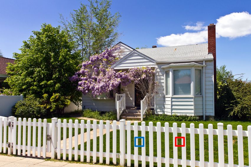
2         Ran Margolin, Lihi Zelnik-Manor, and Ayellet Tal

    In this paper, we focus on low-level representations for scene classification. We
propose a novel local descriptor: Oriented Texture Curves (OTC). The descriptor
is based on three key ideas. (i) A patch contains different information along
different orientations that should be captured. For each orientation we construct
a curve that represents the color variation of the patch along that orientation. (ii)
The shapes of these curves characterize the texture of the patch. We represent
the shape of a curve by its shape properties, which are robust to illumination
differences and geometric distortions of the patch. (iii) Homogeneous patches
require special attention to avoid the creation of false features. We do so by
suggesting an appropriate normalization scheme. This normalization scheme is
generic and can be used in other domains.
    Our main contributions are two-fold. First, we propose a novel descriptor,
OTC, for scene classification. We show that it achieves an improvement of 7.35%
in accuracy over the previously top-performing descriptor, HOG2x2 [5]. Second,
we show that a combination between the HOG2x2 descriptor and our OTC
descriptor results in an 11.6% improvement in accuracy over the previously top-
performing scene classification feature-based algorithm that employs 14 descrip-
tors [34].

2      The OTC Descriptor
Our goal is to design a descriptor that satisfies the following two attributes that
were shown to be beneficial for scene classification [34].

    – Rotational-sensitivity: Descriptors that are not rotationally invariant pro-
      vide better classification than rotationally invariant descriptors [34]. This is
      since scenes are almost exclusively photographed parallel to ground. There-
      fore, horizontal features, such as railings, should be differentiated from ver-
      tical features, such as fences. This is the reason why descriptors, such as
      HOG2x2 [5] and Dense SIFT [13], outperform rotationally invariant descrip-
      tors, such as Sparse SIFT [30] and LBP [20, 1].

    – Texture: The top-ranking descriptors for scene classification are texture-
      based [34]. Furthermore, a good texture-based descriptor should be robust to
      illumination changes, local contrast differences and geometric distortions [19].
      This is since, while different photographs of a common scene may differ in
      color, illumination or spatial layout, they usually share similar, but not iden-
      tical, dominant textures. Thus, the HOG2x2 [5], a texture-based descriptor,
      was found to outperform all other non-texture based descriptors [34].

    In what follows we describe in detail the OTC descriptor, which is based on
our three key ideas and the two desired attributes listed above. In Section 2.1, we
suggest a rotationally-sensitive patch representation by way of multiple curves.
The curves characterize the information contained along different orientations
of a patch. In Section 2.2 we propose a novel curve representation that is robust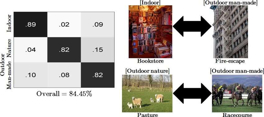
OTC: A Novel Local Descriptor for Scene Classification         3

Fig. 1. OTC overview: Given an image (a), patches are sampled along a dense grid
(b). By traversing each patch along multiple orientations, the patch is represented by
multiple curves (c). Each curve is characterized by a novel curve descriptor that is
robust to illumination differences and geometric distortions (d). The curve descriptor
are then concatenated to form a single descriptor (e). Finally, the OTC descriptor is
obtained by applying a novel normalization scheme that avoids the creation of false
features while offering robustness to local contrast differences (f).

to illumination differences and geometric distortions. Lastly, we concatenate the
obtained multiple curve descriptors into a single descriptor and suggest a novel
normalization scheme that avoids the creation of false features in the descrip-
tors of homogeneous patches (Section 2.3). An overview of our framework is
illustrated in Figure 1.

2.1   Patch to multiple curves

Our first goal is to describe the texture of a given patch. It has been shown that
different features exhibit different dominant orientations [19]. Thus, by examin-
ing a patch along different orientations, different features can be captured.
    To do so, we divide an N × N patch P into N strips along different orienta-
tions (in practice, 8), as shown in Figure 2. For each orientation θ, an N -point
sampled curve cθ is constructed. The ith sampled point along the oriented curve
cθ is computed as the mean value of its ith oriented strip Sθ,i :

                                   1     X
                      cθ (i) =             P (x)   1 ≤ i ≤ N,                     (1)
                                 |Sθ,i |
                                      x∈Sθ,i

|Sθ,i | denoting the number of pixels contained within strip Sθ,i . For an RGB
colored patch, Cθ (i) is computed as the mean RGB triplet of its ith oriented strip
Sθ,i . Note that by employing strips of predefined orientations, regardless of the
input patch, we effectively enforce the desired property of rotational-sensitivity.
4       Ran Margolin, Lihi Zelnik-Manor, and Ayellet Tal

       −90 ◦      −67.5 ◦   −45 ◦   −22.5 ◦    0◦      22.5 ◦    45 ◦     67.5 ◦

Fig. 2. Patch to multiple curves: To represent a patch by multiple curves, we divide
the patch into strips (illustrated above as colored strips) along multiple orientations.
For each orientation, we construct a curve by first “walking” across the strips (i.e.
along the marked black arrows). Then, each point of the curve is defined as the mean
value of its corresponding strip.

            (a)             (b)        Pa1

            (c)             (d)        Pa2

Fig. 3. Illumination differences and geometric distortions: (a-d) Curves ob-
tained along four orientations of two very similar patches, Pa1 & Pa2 (blue for Pa1
and red for Pa2 ). The generated curves are different due to illumination and geometric
differences between the patches. Thus, a more robust curve representation is required.

2.2   Curve descriptor

Our second goal is to construct a discriminative descriptor that is robust to illu-
mination differences and geometric distortions. An example why such robustness
is needed is presented in Figure 3. Two patches were selected. The patches are
very similar but not identical. Differences between them include their illumina-
tion, the texture of the grass, the spacing between the white fence posts, and
their centering. This can be seen by observing their four curves (generated along
four orientations) shown on the left. The differences in illumination can be ob-
served by the difference in heights of the two curves (i.e. the more illuminated
patch Pa1 results in a higher curve than Pa2 ). The geometric differences between
the two patches can be observed in Figure 3(c). Due to the difference in spacing
between the white fence posts, the drop of the red curve is to the left of the
drop of the blue curve. We hence conclude that these curves are not sufficiently
robust to illumination differences and geometric distortions.
      Looking again at Figure 3, it can be seen that while the curves are different,
their shapes are highly similar. To capture the shape of these curves we describe
each curve by its gradients and curvatures. For a gray-level patch, for each curve
cθ we compute its forward gradient c0θ (i) and an approximation of its curvature
c00θ (i) [3] as: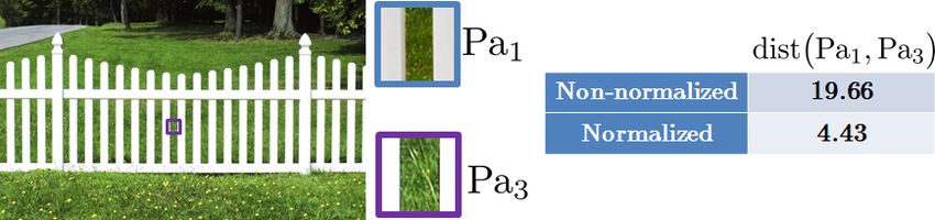
OTC: A Novel Local Descriptor for Scene Classification                      5

Curvature Gradient

                                                                                                  Sorted
                     (a) −90 ◦                 (b) −45 ◦                   (c) 0 ◦   (d) 45 ◦              (e) Sorting of (c)

Fig. 4. Gradients and Curvatures: The resulting gradients and curvatures of the
four curves in Figure 3 (a-d). While offering an improvement in terms of robustness
to illumination differences, this representation is still sensitive to geometric distortions
(c). By applying a sorting permutation, robustness to such distortions is enforced (e).

                                c0θ (i) = cθ (i + 1) − cθ (i)                        1 ≤i < N                          (2)
                                c00θ (i)   =   c0θ (i   + 1) −   c0θ (i)             1 ≤ i < (N − 1).                  (3)

For RGB curves, we define the forward RGB gradient between two points as the
L2 distance between them, signed according to their gray-level gradient:

                      Cθ0 (i) = sign {c0θ (i)} · ||Cθ (i + 1) − Cθ (i)||2                   1 ≤i < N                   (4)
                     Cθ00 (i)   =   Cθ0 (i   + 1) −       Cθ0 (i)                           1 ≤ i < (N − 1).           (5)

      The resulting gradients and curvatures of the four curves shown in Figure 3
are presented in Figure 4(a-d). While offering an improvement in robustness to
illumination differences, the gradients and curvatures in Figure 4(c) still differ.
The differences are due to geometric differences between the patches (e.g. the
centering of the patch and the spacing between the fence posts). Since scenes of
the same category share similar, but not necessarily identical textures, we must
allow some degree of robustness to these types of geometric distortions.
      A possible solution to this could be some complex distance measure be-
tween signals such as dynamic time warping [24]. Apart from the computational
penalty involved in such a solution, employing popular mid-level representations
such as BoW via K-means is problematic when the centroids of samples are
ill-defined. Another solution that has been shown to provide good results are
histograms [2, 10, 17]. While histogram-based representations perform well [19],
they suffer from two inherent flaws. The first is quantization error, which may be
alleviated to some degree with the use of soft-binning. The second flaw concerns
weighted histograms, in which two different distributions may result in identical
representations.
      Instead, we suggest an alternative orderless representation to that of his-
tograms, which involves applying some permutation π to each descriptor Cθ0 and
Cθ00 . Let dsc1 and dsc2 denote two descriptors (e.g. those presented in Figure 4(c)-
top in red and blue). The permutation we seek is the one that minimizes the L1
6 Ran Margolin, Lihi Zelnik-Manor, and Ayellet Tal
Fig. 5. Robustness to local contrast differences: We desire robustness to local
contrast differences, such as those present between Pa1 (from Figure 3) and Pa3 . By
applying a normalization scheme, robustness to such differences is obtained.
distance between them:
π = arg min {||π́(dsc1 ) − π́(dsc2 )||1 } . (6)
π́
A solution to Equation (6) is found in the following theorem, for which we
provide proof in Appendix A.
Theorem 1. The permutation that minimizes the L1 distance between two vec-
tors (descriptors) is the sorting permutation πsort .
That is to say, we sort each gradient (or curvature) in a non-decreasing man-
ner. Sorting has been previously used to achieve rotational invariance [33, 16].
Yet, since our curves are constructed along predefined orientations, we main-
tain the desired attribute of rotational-sensitivity, while achieving robustness to
geometric distortions. Figure 4(e) illustrates the result of sorting the gradients
and curvatures shown in Figure 4(c). It is easy to see that this results in a very
similar response for both patches.
2.3 H-bin normalization
Thus far, we have constructed a robust curve representation. Keeping in mind
our goal of a patch descriptor, we proceed to concatenate the sorted gradients
and curvatures:
OTCNo-Norm = πsort (Cθ0 1 ), πsort (Cθ001 ), . . . , πsort (Cθ0 8 ), πsort (Cθ008 ) .
(7)
While offering a patch descriptor that is robust to illumination differences and
geometric distortions, the descriptor still lacks robustness to local contrast differ-
ences. An example of such differences is illustrated in Figure 5. A similar patch
to that sampled in Figure 3 is sampled from a different image. The patches differ
in their local contrast, therefore they are found to have a large L1 distance.
To support robustness to local contrast differences, we wish to normalize our
descriptor. The importance of an appropriate normalization scheme has been pre-
viously stressed [2]. Examples of normalization schemes include the well knownOTC: A Novel Local Descriptor for Scene Classification 7
Descriptors of a Descriptors of a
textured patch textureless patch L2 -normalized Descriptors
No H-bin
(a) (b) (c)
With H-bin
H-bin H-bin
(d) (e) (f)
Fig. 6. H-bin normalization scheme: Under previous normalization schemes, de-
scriptors of textureless patches (b) are stretched into false features (c)-blue. By adding
a low-valued bin, prior to normalization (d-e), false features are avoided (f)-blue. In
case of a descriptor of a textured patch (d),
the small value hardly affects the normal-
ized result (f)-red compared to (c)-red . The added H-bin may be thought of as a
measure of homogeneity.
L1 and L2 norms, the overlapping normalization scheme [2] and the L2 -Hys nor-
malization [17]. Unfortunately, these schemes fail to address the case of a tex-
tureless patch. Since the OTC descriptor is texture-based, textureless patches
result in a descriptor that contains mostly noise. Examples of such patches can
be found in the sky region in Figure 3.
The problem of normalizing a descriptor of a textureless patch is that its
noisy content is stretched into false features. An example of this can be seen
in Figure 6. The descriptors of a textured patch and a textureless patch are
shown in Figure 6(a-b). Applying L2 normalization to both descriptors results
in identical descriptors (Figure 6(c)).
To overcome this, we suggest a simple yet effective method. For each descrip-
tor, we add a small-valued bin (0.05), which we denote as the Homogeneous-bin
(H-bin). While the rest of the descriptor measures the features within a patch,
the H-bin measures the lack of features therein. We then apply L2 normaliza-
tion. Due to the small value of the H-bin, it hardly affects patches that contain
features. Yet, it prevents the generation of false features in textureless patches.
An example can be seen in Figure 6. An H-bin was added to the descriptor
of both textured and textureless patches (Figure 6(d-e)). After normalization,
the descriptor of the textured patch is hardly affected ((f)-red compared to
(c)-red). Yet, the normalized descriptor of the textureless patch retains its low
valued features. This is while indicating the presence of a textureless patch by
its large H-bin (Figure 6(f)-blue). In Figure 7(b) we present the H-bins of the
L2 -normalized OTC descriptors of Figure 7(a). As expected the sky region is
found as textureless, while the rest of the image is identified as textured.8 Ran Margolin, Lihi Zelnik-Manor, and Ayellet Tal
(a) Input (b) H-bin
Fig. 7. H-bin visualization: (b) The normalized H-bins of the OTC descriptors of
(a). As expected, patches with little texture result in a high normalized H-bin value.
Thus, the final OTC descriptor is obtained by:
H-bin, OTCNo-Norm
OTC = . (8)
H-bin, OTCNo-Norm
2
3 Evaluation
Benchmark: To evaluate the benefit of our OTC descriptor, we test its perfor-
mance on the SUN397 benchmark [34], the most extensive scene classification
benchmark to-date. The benchmark includes 397 categories, amounting to a to-
tal of 108, 574 color images, which is several orders of magnitude larger than
previous datasets. The dataset includes a widely diverse set of indoor and out-
door scenes, ranging from elevator-shafts to tree-houses, making it highly robust
to over-fitting. In addition, the benchmark is well defined with a strict evaluation
scheme of 10 cross-validations of 50 training images and 50 testing images per
category. The average accuracy across all categories is reported.
OTC setup: To fairly evaluate the performance of our low-level representa-
tion, we adopt the simple mid-level representation and learning scheme that
were used in [34]. Given an image, we compute its OTC descriptors on a dense
3 × 3 grid (images were resized to contain no more than 3002 pixels). Each
descriptor is computed on a 13 × 13 sized patch, resulting in a total length of
8 × |{z}
|{z} 12 + |{z} 11 = 184 values per patch. After adding the H-bin and
orientations gradient curvature
normalizing, our final descriptors are of length 185. The local OTC descriptors
are then used in a 3-level Spatial Pyramid Matching scheme (SPM) [13] with
a BoW of 1000 words via L1 K-means clustering. Histogram intersection [13] is
used to compute the distance between two SPMs. Lastly, we use a simple 1-vs-all
SVM classification framework.
In what follows we begin by comparing the classification accuracy of our OTC
descriptor to state-of-the-art descriptors and algorithms (Section 3.1). We then
proceed in Section 3.2 to analyze its classification performance in more detail.OTC: A Novel Local Descriptor for Scene Classification 9
3.1 Benchmark results
To demonstrate the benefits of our low-level representation we first compare our
OTC descriptor to other state-of-the-art low-level descriptors with the common
mid-level representation and a 1-vs-all SVM classification scheme of [34].
In Table 1(left) we present the top-four performing descriptors on the SUN397
benchmark [34]: (1) Dense SIFT [13]: SIFT descriptors are extracted on a dense
grid for each of the HSV color channels and stacked together. A 3-level SPM mid-
level representation with a 300 BoW is used. (2) SSIM [26]: SSIM descriptors
are extracted on a dense grid and quantized into a 300 BoW. The χ2 distance
is used to compute the distance between two spatial histograms. (3) G-tex [34]:
Using the method of [9], the probability of four geometric classes are computed:
ground, vertical, porous and sky. Then, a texton histogram is built for each
class, weighted by the probability that it belongs to that geometric class. The
histograms are normalized and compared with the χ2 distance. (4) HOG2x2 [5]:
HOG descriptors are computed on a dense grid. Then, 2×2 neighboring HOG de-
scriptors are stacked together to provide enhanced descriptive power. Histogram
intersection is used to compute the distance between the obtained 3-level SPMs
with a 300 BoW.
As shown in Table 1, our proposed OTC descriptor significantly outperforms
previous descriptors. We achieve an improvement of 7.35% with a 1000 BoW
and an improvement of 3.98% with a 300 BoW (denoted OTC-300).
Table 1. SUN397 state-of-the-art performance: Left: Our OTC descriptor out-
performs all previous descriptors. Right: Performance of more complex state-of-the-art
algorithms. Our simple combination of OTC and HOG2x2 outperforms most of the
state-of-the-art algorithms
Descriptors Algorithms
Name Accuracy Name Accuracy
Dense SIFT [13] 21.5 ML-DDL [27] 23.1
SSIM [26] 22.5 S-Manifold [12] 28.9
G-tex [34] 23.5 OTC 34.56
HOG2x2 [5] 27.2 contextBow-m+semantic [31] 35.6
OTC-300 31.18 14 Combined Features [34] 38
OTC 34.56 DeCAF [4] 40.94
OTC + HOG2x2 49.6
MOP-CNN [7] 51.98
Since most recent works deal with mid-level representations, high-level rep-
resentations and learning schemes, we further compare in Table 1(right) our
descriptor to more complex state-of-the-art scene classification algorithms: (1)
ML-DDL [27] suggests a novel learning scheme that takes advantage of the hi-
erarchical correlation between scene categories. Based on densely sampled SIFT
descriptors a dictionary and a classification model are learned for each hierar-10 Ran Margolin, Lihi Zelnik-Manor, and Ayellet Tal
chy (3 hierarchies are defined for the SUN397 dataset [34]). (2) S-Manifold [12]
suggests a mid-level representation that combines the SPM representation with
a semantic manifold [25]. Densely samples SIFT descriptors are used as local
descriptors. (3) contextBoW-m+semantic [31] suggests both mid-level and high-
level representations in which pre-learned context classifiers are used to construct
multiple context-based BoWs. Five local features are used (four low-level and
one high-level): SIFT, texton filterbanks, LAB color values, Canny edge de-
tection and the inferred semantic classification. (4) 14 Combined Features [34]
combines the distance kernels obtained by 14 descriptors (four of which appear
in Table 1(left)). (5,6) DeCAF [4] & MOP-CNN [7] both employ a deep convo-
lutional neural network.
In Table 1(right) we show that by simply combining the distance kernels
of our OTC descriptor and those of the HOG2x2 descriptor (at a 56-44 ratio),
we outperform most other more complex scene classification algorithms. A huge
improvement of 11.6% over the previous top performing feature-based algorithm
is achieved. A nearly comparable result is achieved when compared to MOP-
CNN that is based on a complex convolutional neural network.
For completeness, in Table 2 we compare our OTC descriptor on two addi-
tional smaller benchmarks: the 15-scene dataset [13] and the MIT-indoor dataset [23].
In both benchmarks, our simplistic framework outperforms all other descriptors
in similar simplistic frameworks. Still, several state-of-the-art complex methods
offer better performance than our framework. We believe that incorporating our
OTC descriptor into these more complex algorithms would improve their per-
formance even further.
Table 2. 15-scene & MIT-indoor datasets: Our OTC descriptor outperforms pre-
vious descriptors and is comparable with several more complex methods
15-scene MIT-indoor
Name Accuracy Name Accuracy
SSIM [26] 77.2 SIFT [13] 34.40
G-tex [34] 77.8 Discriminative patches [28] 38.10
HOG2x2 [5] 81.0 OTC 47.33
SIFT [13] 81.2 Disc. Patches++ [28] 49.40
OTC 84.37 ISPR + IFV [15] 68.5
ISPR + IFV [15] 91.06 MOP-CNN [7] 68.88
3.2 Classification analysis
In what follows we provide an analysis of the classification accuracy of our de-
scriptor on the top two hierarchies of the SUN397 dataset. The 1st level consists
of three categories: indoor, outdoor nature and outdoor man-made. The 2nd level
consists of 16 categories (listed in Figure 9).OTC: A Novel Local Descriptor for Scene Classification 11
Fig. 8. 1st level confusion matrix: Left: The confusion matrix of our OTC descriptor
on the 1st level of the SUN397 dataset shows that most misclassifications occur between
indoor & outdoor man-made scenes, and within the two types of outdoor scenes. Right:
Images in which the classification was mistakingly swapped.
In Figure 8(left) we present the confusion matrix on the 1st level of the
SUN397 dataset for which an impressive 84.45% success rate is achieved (com-
parison to other methods is shown later). Studying the matrix, confusion is
mostly apparent between indoor & outdoor man-made scenes and within the
two types of outdoor scenes. Misclassification between indoor and outdoor man-
made scenes is understandable, since both scene types consist of similar textures
such as straight horizontal and vertical lines, as evident by comparing the im-
age of the Bookstore scene to that of the Fire-escape Figure 8(top-right) .
Differences between outdoor nature scenes and outdoor man-made scenes are
often contextual, such as the Pasture and Racecourse images shown in Fig-
ure 8(bottom-right). Thus, it is no surprise that a texture-based classification
may confuse between the two.
The 2nd level confusion matrix is displayed in Figure 9. Our average success
rate is 57.2%. Most confusions occur between categories of similar indoor or
outdoor settings. Furthermore, we note that the two categories with the highest
errors are Commercial Buildings and House, Garden & Farm. The former is
mostly confused with Historical Buildings and the latter with Forests & Jungle.
These understandable semantic confusions further confirm the robustness of the
classification strength of our OTC descriptor.
Lastly, we compare in Table 3 the average classification accuracy of our OTC
descriptor on each of the three hierarchical levels, to that of ML-DDL [27].
ML-DDL is the best performing algorithm to reports results on the different
hierarchies. In all three levels our descriptor outperforms the results of ML-DDL,
which utilizes a hierarchical based learning framework.12 Ran Margolin, Lihi Zelnik-Manor, and Ayellet Tal
Overall=57.2%
Fig. 9. 2nd level confusion matrix: The confusion matrix of our OTC descriptor
on the 2nd level of the SUN397 dataset shows that most confusions occur between
categories of similar indoor or outdoor settings. Furthermore, most confusions occur
between classes of semantic differences such as Home & Hotel and Workplace. These
understandable misclassifications further confirm the strength of our OTC descriptor
at capturing similar textures.
Table 3. SUN397 hierarchical classification: Our OTC descriptor outperforms
the hierarchical based learning framework of [27] on all of the three hierarchical levels
of the SUN397 dataset
Accuracy
Name
1st 2nd 3rd
ML-DDL [27] 83.4 51 23.1
OTC 84.45 57.2 34.56
4 Conclusion
We presented the OTC descriptor, a novel low-level representation for scene
classification. The descriptor is based on three main ideas. First, representing
the texture of a patch along different orientations by the shapes of multiple
curves. Second, using sorted gradients and curvatures as curve descriptors, which
are robust to illumination differences and geometric distortions of the patch.
Third, enforcing robustness to local contrast differences by applying a novel
normalization scheme that avoids the creation of false features.
Our descriptor achieves an improvement of 7.35% in accuracy over the previ-
ously top-performing descriptor, on the most extensive scene classification bench-
mark [34]. We further showed that a combination between the HOG2x2 descrip-
tor [5] and our OTC descriptor results in an 11.6% improvement in accuracyOTC: A Novel Local Descriptor for Scene Classification 13
over the previously top-performing scene classification feature-based algorithm
that employs 14 descriptors.
Acknowledgments: This research was funded (in part) by the Intel Collabora-
tive Research Institute for Computational Intelligence (ICRI–CI), Minerva, the
Ollendorff Foundation, and the Israel Science Foundation under Grant 1179/11.
A Proof of Theorem 1
Theorem 1. The permutation that minimizes the L1 distance between two vec-
tors (descriptors) is the sorting permutation πsort .
Proof. Let á1×N and b́1×N be two vectors of length N . We apply permutation πb
that sorts the elements of b́1×N to both vectors á1×N and b́1×N . Note that ap-
plying this permutation to both vectors a1×N = πb (á1×N ) , b1×N = πb (b́1×N )
does not change their L1 distance.
Proof by induction on the length of the vectors, N :
For the basis of the induction let N = 2. Let xi denote the ith element in vector
x. Below we provide proof for the case of a1 ≤ a2 (Recall that b1 ≤ b2 ). A similar
proof can be done for a2 ≤ a1 .
We show that |b1 − a1 | + |b2 − a2 | ≤ |b1 − a2 | + |b2 − a1 |:
| {z } | {z }
LH RH
(b1 ≤ b2 ≤ a1 ≤ a2 ) : LH = a1 + a2 − b1 − b2 = RH (9)
(b1 ≤ a1 ≤ b2 ≤ a2 ) : LH = a1 − b2 + a2 − b1 ≤ = b2 − a1 + a2 − b1 = RH (10)
|{z}
a1 ≤b2
(b1 ≤ a1 ≤ a2 ≤ b2 ) : LH = a1 − b1 + b2 − a2 ≤ a2 − b1 + b2 − a1 = RH (11)
|{z}
a1 ≤a2
(a1 ≤ b1 ≤ b2 ≤ a2 ) : LH = b1 − a1 + a2 − b2 ≤ b2 − a1 + a2 − b1 = RH (12)
|{z}
b1 ≤b2
(a1 ≤ b1 ≤ a2 ≤ b2 ) : LH = b1 − a1 + b2 − a2 ≤ a2 − a1 + b2 − b1 = RH (13)
|{z}
b1 ≤a2
(a1 ≤ a2 ≤ b1 ≤ b2 ) : LH = b1 + b2 − a1 − a2 = RH (14)
Now suppose that the theorem holds for N < K. We prove that it holds for
N = K.
First, we prove that given a permutation π that minimizes ||b − π(a)||1 ⇒ π
is the sorting permutation πsort .
Let π be some permutation applied to a, so that a minimal L1 distance is
achieved:
π = arg min {||b − π(a)||1 } . (15)
π14 Ran Margolin, Lihi Zelnik-Manor, and Ayellet Tal
Let xi:j denote a sub-vector of a vector x from index i to index j.
We can decompose D = ||b−π(a)||1 into D = ||b1 − π(a)1 ||1 + ||b2:K − π(a)2:K ||1 .
| {z } | {z }
D1 D2:K
The minimality of D infers the minimality of D2:K . Otherwise, a smaller L1 dis-
tance can be found by reordering the elements of π(a)2:K , contradicting the
minimality of D. Following our hypothesis, we deduce that π(a)2:K is sorted.
Specifically π(a)2 = min{π(a)2:K }.
Similarly, by decomposing D into D = ||b1:(K−1) − π(a)1:(K−1) ||1 + ||bK − π(a)K ||1
| {z } | {z }
D1:(K−1) DK
we deduce that π(a)1 = min{π(a)1:(K−1) } ≤ π(a)2 .
This implies, that π(a) is sorted and that π = πsort .
Next, we prove the other side, i.e. if π = πsort ⇒ π minimizes ||b − π(a)||1 .
Assume to the contrary that there exists a non-sorting permutation πmin 6= πsort
that can achieve a minimal L1 distance D0 , which is smaller than D = ||b −
πsort (a)||1 . Then, there must be at least two elements πmin (a)i > πmin (a)j that
are out of order (i.e. i < j).
We can decompose D0 into:
X
D0 = |bk − πmin (a)k | + ||(bi , bj ) − (πmin (a)i , πmin (a)j )||1 . (16)
k6=i,j
(17)
Yet, as proved in the basis of our induction, the following inequality is true:
||(bi , bj ) − (πmin (a)i , πmin (a)j )||1 |{z}
< ||(bi , bj ) − (πmin (a)j , πmin (a)i )||1 . (18)
πmin (a)jOTC: A Novel Local Descriptor for Scene Classification 15
5. Felzenszwalb, P.F., Girshick, R.B., McAllester, D., Ramanan, D.: Object detection
with discriminatively trained part-based models. PAMI 32(9), 1627–1645 (2010)
6. Gao, T., Koller, D.: Discriminative learning of relaxed hierarchy for large-scale
visual recognition. In: ICCV. pp. 2072–2079 (2011)
7. Gong, Y., Wang, L., Guo, R., Lazebnik, S.: Multi-scale orderless pooling of deep
convolutional activation features. CoRR (2014)
8. Hays, J., Efros, A.A.: Im2gps: estimating geographic information from a single
image. In: CVPR. pp. 1–8 (2008)
9. Hoiem, D., Efros, A.A., Hebert, M.: Recovering surface layout from an image. IJCV
75(1), 151–172 (2007)
10. Koenderink, J.J., Van Doorn, A.J.: The structure of locally orderless images. IJCV
31(2-3), 159–168 (1999)
11. Krapac, J., Verbeek, J., Jurie, F.: Modeling spatial layout with fisher vectors for
image categorization. In: ICCV. pp. 1487–1494 (2011)
12. Kwitt, R., Vasconcelos, N., Rasiwasia, N.: Scene recognition on the semantic man-
ifold. In: ECCV. pp. 359–372 (2012)
13. Lazebnik, S., Schmid, C., Ponce, J.: Beyond bags of features: Spatial pyramid
matching for recognizing natural scene categories. In: CVPR. pp. 2169–2178 (2006)
14. Li, Q., Wu, J., Tu, Z.: Harvesting mid-level visual concepts from large-scale internet
images. In: CVPR. pp. 851–858 (2013)
15. Lin, D., Lu, C., Liao, R., Jia, J.: Learning important spatial pooling regions for
scene classification. In: CVPR (2014)
16. Liu, L., Fieguth, P., Kuang, G., Zha, H.: Sorted random projections for robust
texture classification. In: ICCV. pp. 391–398 (2011)
17. Lowe, D.G.: Object recognition from local scale-invariant features. In: ICCV. vol. 2,
pp. 1150–1157 (1999)
18. Meng, X., Wang, Z., Wu, L.: Building global image features for scene recognition.
Pattern Recognition 45(1), 373–380 (2012)
19. Mikolajczyk, K., Schmid, C.: A performance evaluation of local descriptors. PAMI
27(10), 1615–1630 (2005)
20. Ojala, T., Pietikainen, M., Maenpaa, T.: Multiresolution gray-scale and rotation
invariant texture classification with local binary patterns. PAMI 24(7), 971–987
(2002)
21. Oliva, A., Torralba, A.: Modeling the shape of the scene: A holistic representation
of the spatial envelope. IJCV 42(3), 145–175 (2001)
22. Oliva, A., Torralba, A.: The role of context in object recognition. Trends in cogni-
tive sciences 11(12), 520–527 (2007)
23. Quattoni, A., Torralba, A.: Recognizing indoor scenes. In: CVPR (2009)
24. Rabiner, L.R., Juang, B.H.: Fundamentals of speech recognition. Prentice Hall
(1993)
25. Rasiwasia, N., Vasconcelos, N.: Scene classification with low-dimensional semantic
spaces and weak supervision. In: CVPR. pp. 1–6 (2008)
26. Shechtman, E., Irani, M.: Matching local self-similarities across images and videos.
In: CVPR. pp. 1–8 (2007)
27. Shen, L., Wang, S., Sun, G., Jiang, S., Huang, Q.: Multi-level discriminative dic-
tionary learning towards hierarchical visual categorization. In: CVPR. pp. 383–390
(2013)
28. Singh, S., Gupta, A., Efros, A.: Unsupervised discovery of mid-level discriminative
patches. In: ECCV, pp. 73–86 (2012)
29. Sivic, J., Zisserman, A.: Video google: A text retrieval approach to object matching
in videos. In: ICCV. pp. 1470–1477 (2003)16 Ran Margolin, Lihi Zelnik-Manor, and Ayellet Tal
30. Sivic, J., Zisserman, A.: Video data mining using configurations of viewpoint in-
variant regions. In: CVPR. pp. I–488 (2004)
31. Su, Y., Jurie, F.: Improving image classification using semantic attributes. IJCV
100(1), 59–77 (2012)
32. Vogel, J., Schiele, B.: Semantic modeling of natural scenes for content-based image
retrieval. IJCV 72(2), 133–157 (2007)
33. Wang, Z., Fan, B., Wu, F.: Local intensity order pattern for feature description.
In: ICCV. pp. 603–610 (2011)
34. Xiao, J., Hays, J., Ehinger, K.A., Oliva, A., Torralba, A.: Sun database: Large-scale
scene recognition from abbey to zoo. In: CVPR. pp. 3485–3492 (2010)
35. Yang, J., Yu, K., Gong, Y., Huang, T.: Linear spatial pyramid matching using
sparse coding for image classification. In: CVPR. pp. 1794–1801 (2009)You can also read