CNN based ecient image classication system for smartphone device
←
→
Page content transcription
If your browser does not render page correctly, please read the page content below
CNN based e cient image classi cation system for smartphone device Mayank Mishra University of Petroleum and Energy Studies, Dehradun, India Tanupriya Choudhury ( tanupriya1986@gmail.com ) University of Petroleum and Energy Studies, Dehradun, India Tanmay Sarkar ( tanmays468@gmail.com ) Malda Polytechnic, West Bengal State Council of Technical Education, Govt. of West Bengal, Malda-732 102, India Research Article Keywords: Deep Learning, Convolutional Neural Network, Transfer Learning Posted Date: April 17th, 2021 DOI: https://doi.org/10.21203/rs.3.rs-428430/v1 License: This work is licensed under a Creative Commons Attribution 4.0 International License. Read Full License
Electronic Letters on Computer Vision and Image Analysis 0(0):1-7, 2021

 CNN based efficient image classification system for smartphone
                           device
                        Mayank Mishra1 , Tanupriya Choudhury1∗ and Tanmay Sarkar2

         1
           School of Computer Science, University of Petroleum and Energy Studies, Dehradun, Uttarakhand, India
   2
       Malda Polytechnic, West Bengal State Council of Technical Education, Govt. of West Bengal, Malda-732102, India
                                   ∗
                                     Corresponding author: tanupriya1986@gmail.com

                                                         Abstract
            In our work, we look to classify images that make their way into our smartphone devices through var-
        ious social-media text-messaging platforms. We aim at classifying images into three broad categories:
        document-based images, quote-based images, and photographs. People, especially students, share many
        document-based images that include snapshots of essential emails, handwritten notes, articles, etc. Quote-
        based images, consisting of birthday wishes, motivational messages, festival greetings, etc., are among the
        highly shared images on social media platforms. A significant share of images constitutes photographs of
        people, including group photographs, selfies, portraits, etc. We train various convolutional neural network
        (CNN) based models on our self-made dataset and compare their results to find our task’s optimum model.

        Key Words: Deep Learning, Convolutional Neural Network, Transfer Learning.

1 Introduction
In the current time, a plethora of images get shared across various social media platforms that help us discover
other people, new ideas, concepts, and information. Many images make way into our smartphone devices as a
result of active participation on such platforms. We have recognized the images to fall broadly under three main
categories, namely, document-based images, which consists of snapshots of essential emails, handwritten notes,
articles, etc., quote-based images, which includes images of birthday wishes, motivational messages, festival
greetings, etc., and photographs, which constitutes of photographs of people, including group photographs,
selfies, portraits, etc. We focus on implementing a deep learning-based classification system to automatically
group an image into one of the three categories mentioned above.
   Deep learning is a machine learning technique that teaches a model to learn by examples. The models are
trained on a large set of data (like images, text, sound, etc.) using neural network architectures, which allows
them to perform classification tasks based on what they learned from the training. Such models achieve high
performance even with a small training set when designed with appropriate settings.
   In deep learning, researchers have extensively used CNN for many pattern recognition problems, especially
image recognition. It is a specialized type of neural network with convolutional layers that learn highly spe-
cific features from input images. In 2012, (Krizhevsky, Sutskever, & Hinton, 2012) won the ImageNet Large
   Correspondence to:
   Recommended for acceptance by
   ELCVIA ISSN:1577-5097
   Published by Computer Vision Center / Universitat Autònoma de Barcelona, Barcelona, Spain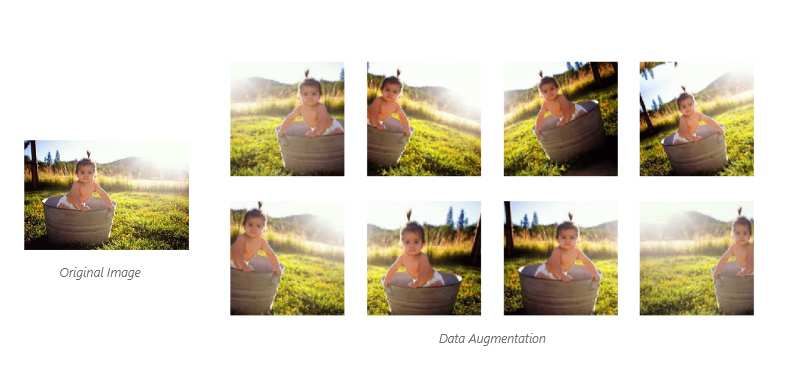
2               Name1 et al. / Electronic Letters on Computer Vision and Image Analysis 0(0):1-7, 2021

Scale Visual Recognition Challenge (ILSVRC) by training a CNN with five convolution layers and three fully-
connected (FC) layers and ReLU activation function. After the success of AlexNet, (Zeiler & Fergus, 2013)
proposed the ZFNet that made several changes in the hyperparameters of the network and performed even
better. Following that, (Szegedy et al., 2015) presented the GoogLeNet that won the ILSVRC in 2014. The net-
work consisted of a deep 22 layer CNN but a reduced number of parameters than the AlexNet. In the same year,
(Simonyan & Zisserman, 2015) put forward the VGGNet, which stood second after GoogLeNet and gained a
lot of popularity. The VGG16 network had sixteen layers and five blocks, and the VGG19 network had 19
layers with extra convolution layers in the last three blocks. (He, Zhang, Ren, & Sun, 2016)’s ResNet won the
ILSVRC in 2015 by introducing skip connections in a very deep network of 152 layers.
   While working with our relatively smaller dataset, we took the assistance of transfer learning which pre-
vented our model from learning everything from scratch and allowed the optimization process to be fast. To
provide the best possible model for our classification task, we created five models and compared their results
on our self-modeled dataset. The model that used VGG16 as a feature extractor recorded the highest accuracy
rate of 95%.

2 Literature Review
During the early 1900s, the convolutional networks introduced by (LeCun et al., 1989) exhibited high perfor-
mance at the tasks of hand-written digit classification and face detection. The network’s use during this period
was one of the first times when neural networks had undertaken real-world applications. The development of
GPUs ensured CNN became the go-to solution for image classification tasks in the upcoming years. Work by
(Ciregan, Meier, & Schmidhuber, 2012) showcased that they could be applied to tackle much more challenging
visual classification tasks. The network gave state-of-the-art results on NORB and CIFAR-10 datasets. Most
notably, it was the convolutional neural network (CNN) trained by (Krizhevsky et al., 2012) which acted as one
of the most significant breakthroughs in deep learning.
   In 2010, their deep CNN architecture performed amazingly well at the ImageNet Large Scale Visual Recog-
nition Challenge (ILSVRC) that required the architecture to classify 1.2 million high-resolution images into
1000 different categories. Their network architecture included five convolutional layers along with two glob-
ally connected layers with a final 1000-way softmax. This network with 60 million parameters and 500,000
neurons achieved top-1 and top-5 error rates of 39.7% and 18.9%, respectively, on the test data. This model’s
variant was used again in the ILSVRC-2012 competition and achieved a mindblowing top-5 test error rate of
15.3%, with the second-best model achieving a 26.2% error rate.
   But one thing that was not noticed in work by (Krizhevsky et al., 2012) was a clear understanding of why
the classifier did such a good job. (Zeiler & Fergus, 2013) addressed these issues by using a visualization
technique to get insights regarding the intermediate feature layers’ functions and the classifier’s operation.
They also proposed the ZFNet that made several changes in the hyperparameters of (Krizhevsky et al., 2012)’s
network and performed even better.
   Since then, many architectures using CNN have given outstanding results on image classification tasks. In
2014, GoogLeNet by (Szegedy et al., 2015) won the ILSVRC. It was a 22 layer CNN that recorded a top 5 error
rate of 6.7%. GoogLeNet used 12 times fewer parameters than the AlexNet and gave an almost human-like
performance. This network architecture did not use fully-connected layers. Instead, they used an average pool
to go from a 7x7x1024 volume to a 1x1x1024 volume which helped reduce their number of parameters.
   In the same year, (Simonyan & Zisserman, 2015)’s VGGNet secured second place after GoogLeNet at the
ILSVRC-2014’s image classification track. This simple network architecture had a 16 (for VGG16) or a 19
(for VGG19) layer CNN that strictly used 3x3 filters with stride and pad of 1, along with 2x2 max-pooling
layers with stride 2. This network also worked amazingly well for localization tasks and won the first prize at
ILSVRC-2014 in image localization. In the subsequent year, the ResNet architecture developed by (He et al.,
2016) broke the assumption that very deep networks are extremely difficult to train. This network introduced

Name1 et al. / Electronic Letters on Computer Vision and Image Analysis 0(0):1-7, 2021                    3

the use of a residual learning framework to train networks much deeper than before easily. This network of 152
layers won the ILSVRC-2015 with an incredible error rate of 3.6%.
   While these models worked well on the large training datasets, it was still unclear if they would train well
on small training datasets. Datasets like CIFAR-10 rarely took advantage of the depth of the models because of
overfitting. (Liu & Deng, 2015) proposed a modified VGG-16 network, in which by adding stronger regularizer
and Batch Normalization, they achieved an error rate of 8.45% on CIFAR-10 without severe overfitting. This
publication was essential for it to bring forward the idea that if a model is strong enough to fit a large dataset, it
can fit a small dataset too.
   Due to these advancements and refinements, CNN became a favorite for solving complex image classification
problems and opened up a whole new dimension of use. For example, (Levine, Pastor, Krizhevsky, Ibarz,
& Quillen, 2018) used CNN to create hand-eye coordination for robotic grasping. A large CNN trained on
monocular images to predict the probability of whether a task space motion of a robotic gripper will lead to a
successful grasp. The network learned the spatial relationship between the gripper and the objects, thus learning
hand-eye coordination and performing successful grips in real life.
   Similarly, (Kölsch, Afzal, Ebbecke, & Liwicki, 2017) presented a way for real-time training and testing for
document image classification. They used a deep network for feature extraction followed by Extreme Learning
Machines (ELM) for classification. The modification assisted in reducing the time consumed in the training
process.
   In the following years, many modifications and extra functionalities were used with the CNN to perform
image classification for specific tasks. (Tianyu, Zhenjiang, & Jianhu, 2018) mentioned that even though CNN
had achieved high image classification performance, handcrafted features were still essential as they helped de-
scribe images from specific aspects and help CNN in classification tasks. They explored feature fusion methods
and proposed methods to combine CNN with the handcrafted features and achieved significant improvement in
the results.
   (Song et al., 2018) brought forward the problem that CNN had performed wonderfully on single-label image
classification, but CNN for multi-label images was still an issue. They proposed a deep multi-modal CNN for
multi-instance multi-label image classification, called MMCNN-MIML. By putting together CNN and multi-
instance multi-label (MIML) learning, the model represented each image as a bunch of instances for image
classification and has the merits of both CNN and MIML.
   Due to the gaining popularity of CNN, researchers came up with ways to implement the network with ease.
Usually, in state-of-the-art CNNs, their architecture was manually built. Thus, it was difficult for people with
limited knowledge to create their architecture to suit their image classification problem. (Sun, Xue, Zhang,
Yen, & Lv, 2020) proposed a way to generate CNN architecture using genetic algorithms automatically. This
proposal allowed users to get a good CNN architecture for their image classification problem even if they did
not have strong domain knowledge of CNN.
   Many researchers have implemented CNN-based models to tackle different real-world scenarios. (Zhao,
Hao, He, Tang, & Wei, 2020) implemented a visual long-short-term memory(LSTM)based integrated CNN
model for fabric defect image classification. (Gour, Jain, & Sunil Kumar, 2020) designed a residual learning-
based 152 layered CNN named ResHist for breast cancer histopathological image classification.
   After analyzing the past work done in the field of image classification, CNN has emerged as the top priority
for it has given successful results over the years. We thus choose to use CNN for our image classification
problem.
4      Name1 et al. / Electronic Letters on Computer Vision and Image Analysis 0(0):1-7, 2021

    Author(s)                  Title                 Focus Area              Main Idea/Result
    (LeCun et           al.,   Backpropagation       Convolutional Net-      Applied convolu-
    1989)                      applied to hand-      work                    tional networks to
                               written zip code                              the task of recog-
                               recognition                                   nizing handwritten
                                                                             characters
    (Ciregan    et      al.,   Multi-column          Image classifica-       Improved the im-
    2012)                      deep neural net-      tion, CNN               plementation        of
                               works for image                               CNN and recorded
                               classification                                better performance
                                                                             on MNIST, NORB
                                                                             and CIFAR-10
    (Krizhevsky et al.,        ImageNet Classifi-    Image classifica-       Created a deep
    2012)                      cation with Deep      tion, CNN               CNN         architec-
                               Convolutional                                 ture that won the
                               Neural Networks                               ILSVRC-2012 by
                                                                             recording a top-5
                                                                             error rate of 15.3%
    (Zeiler & Fergus,          Visualizing   and     Multi-layered De-       Created a visual-
    2013)                      Understanding         convolutional Net-      ization technique to
                               Convolutional         work (deconvnet)        better understand
                               Networks                                      the       classifier’s
                                                                             working           and
                                                                             to improve the
                                                                             network
    (Szegedy    et      al.,   Going Deeper With     Image       classifi-   Created a 22 layer
    2015)                      Convolutions          cation,       object    network        while
                                                     detection, CNN          keeping the com-
                                                                             putational budget
                                                                             constant and won
                                                                             the ILSVRC 2014
                                                                             with a top 5 error
                                                                             rate of 6.7%
    (Simonyan & Zis-           Very Deep Convo-      Image       classifi-   Created a 16-19
    serman, 2015)              lutional Networks     cation,       object    layer CNN that
                               for     Large-Scale   localization, CNN       strictly used 3x3
                               Image Recognition                             filters with stride
                                                                             and pad of 1,
                                                                             along with 2x2
                                                                             max-pooling layers
                                                                             with stride 2
    (He et al., 2016)          Deep      Residual    Image classifica-       Created a 152 layer
                               Learning for Image    tion, residual block    CNN using resid-
                               Recognition           ,object detection,      ual blocks that won
                                                     object localization,    ILSVRC 2015 with
                                                     CNN                     an error rate of
                                                                             3.6%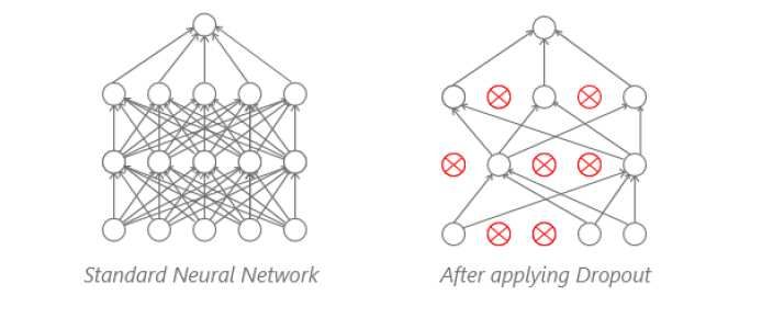
Name1 et al. / Electronic Letters on Computer Vision and Image Analysis 0(0):1-7, 2021        5

(Liu &          Deng,    Very deep convo-         Image classifica-    Proposed a mod-
2015)                    lutional neural net-     tion, CNN            ified      VGG-16
                         work based image                              that achieved an
                         classification using                          8.45% error rate on
                         small training sam-                           CIFAR-10 without
                         ple size                                      severe overfitting
(Levine    et     al.,   Learning hand-eye        CNN                  Used CNN to teach
2018)                    coordination       for                        a robotic gripper
                         robotic     grasping                          hand eye coordina-
                         with deep learning                            tion for successful
                         and       large-scale                         gripping in real life
                         data collection
(Kölsch   et     al.,   Real-time        doc-    CNN, ELM             Created a doc-
2017)                    ument          image                          ument         image
                         classification using                          classification using
                         deep CNN and                                  Deep CNN and
                         extreme learning                              ELM
                         machines
(Tianyu    et     al.,   Combining         cnn    CNN,         Hand    Created a frame-
2018)                    with hand-crafted        Crafted Features     work      to     fuse
                         features for image                            handcrafted       fea-
                         classification                                tures with CNN to
                                                                       get better result
(Song et al., 2018)      A deep multi-            MMCNN-MIML           Put          together
                         modal CNN for                                 CNN and multi-
                         multi-instance                                instance       multi-
                         multi-label image                             label       (MIML)
                         classification                                learning for multi-
                                                                       label image-based
                                                                       classification
(Sun et al., 2020)       Automatically            CNN, genetic algo-   Proposed a way to
                         designing       CNN      rithms               automatically build
                         architectures using                           an architecture of
                         the genetic algo-                             CNN for a partic-
                         rithm for image                               ular image classifi-
                         classification                                cation problem
(Zhao et al., 2020)      A visual long-           VLSTM integrated     Inspired by the
                         short-term memory        CNN                  human          visual
                         based      integrated                         perception        and
                         CNN model for                                 visual      memory
                         fabric defect image                           mechanism,         the
                         classification                                paper proposed a
                                                                       VLSTM integrated
                                                                       CNN model for
                                                                       fabric defect image
                                                                       classification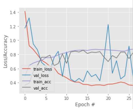
6               Name1 et al. / Electronic Letters on Computer Vision and Image Analysis 0(0):1-7, 2021

             (Gour et al., 2020)   Residual     learn-     Residual learning-     Designed residual
                                   ing based CNN           based CNN              learning-based
                                   for breast cancer                              152 layered CNN
                                   histopathological                              named      ResHist
                                   image classifica-                              for breast cancer
                                   tion                                           histopathological
                                                                                  image classifica-
                                                                                  tion
                                      Table 1: Summary of related works

3 Materials and methods
The work has been achieved by a four-phase approach. We have created five different models using various
network architectures and deep learning concepts that follow the same flow of approach. The optimum model
for the task is determined by drawing a comparison between the performance of each model.

3.1     The four phase approach
The four phases used to achieve the work consist of data collection, preprocessing, training, and evaluation.
[Figure 1] represents the proposed flow of the system.

                                   Figure 1: The proposed system workflow

3.1.1    Data collection
We created our own dedicated dataset from scratch by using the internet as our primary source. The dataset
consists of 969 document-based images, 939 quote-based images, and 960 photographs. Almost all possible
variations within a category are acknowledged. Document-based images include handwritten text, manuscripts,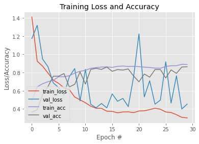
Name1 et al. / Electronic Letters on Computer Vision and Image Analysis 0(0):1-7, 2021            7

typed text, and number sheets. Similarly, photographs are a collection of selfies, group photographs, portraits.
Quote-based images constitute of motivational quotes, birthday wishes, and festival wishes.

3.1.2   Data preprocessing
The high-resolution images were downscaled to 224*224 size. The normalization of images was done based
on the stats of RGB channels from the ImageNet dataset. The data was then split into a training and testing set
that held 2294 and 574 images, respectively.

3.1.3   Training
Post data collection and preprocessing, various models were designed for our specific classification require-
ment. It included defining an architecture, setting an optimizer and loss function, choosing hyperparameters.
After the models were built, they were trained on the training set to make them attain the ability to learn and
perform classification tasks.

3.1.4   Evaluation
Once the models were trained, their performance was recorded by evaluating the models on the testing set
images. The accuracy metric was used to determine the performance of the model. The metric indicated how
good the model trained by measuring the correct predictions made to the total number of predictions.

3.2     Models
3.2.1   Baseline
The baseline model follows a simple CNN architecture that is defined in [Figure 2]. The activation function
used is the ReLU function, and the softmax activation function is used at the end of the network architecture to
make the final predictions. Stochastic gradient descent (SGD) is used as the optimizer with a 1e-4 learning rate
and 0.9 momentum along with categorical crossentropy as the loss function. The model is run for a total of 20
epochs.

                                 Figure 2: Network architecture of baseline model

3.2.2   Baseline + Batch Normalization + Dropout
This model follows the same architecture as the baseline model and integrates several other concepts and
algorithms to improve on the previous model’s performance.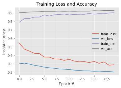
8               Name1 et al. / Electronic Letters on Computer Vision and Image Analysis 0(0):1-7, 2021

   (Ioffe & Szegedy, 2015)’s batch normalization is applied after every ReLU activation layer in the network
before flattening to fully-connected layers. It normalizes the hidden layers’ activation values so that the values’
distribution remains the same during the training. During training time, Batch Normalization calculates the
batch mean [eq. 1] and batch variance [eq. 2] of the layers’ input.
                                                            m
                                                      1 X 2
                                                 µB =    xi                                                    (1)
                                                      m
                                                            i=1
                                                       m
                                                   1 X
                                             2
                                            σB =       (xi − µB )2                                             (2)
                                                   m
                                                      i=1

Post this, normalization is done by subtracting the value and the mean and dividing it by the standard deviation.
                                                                       2 turns out to be 0 in some estimates [eq.
ǫ is added in the denominator to add numerical stability just in case σB
3].
                                                       xi − µB
                                                 xi = q                                                       (3)
                                                           2
                                                         σB + ǫ

Finally, scaling and shifting is performed to achieve the output from the layer [eq. 4].

                                                   yi = γxi + β                                                (4)

The γ and β in [eq. 4] are learned during training along with the parameters of the network.
   Proposed by (Srivastava, Hinton, Krizhevsky, Sutskever, & Salakhutdinov, 2014), dropout removes a few
activations at random from within a mini-batch that is going through, and then from the next, keeps the pre-
vious ones and removes the others. This process prevents the activation from learning some particular part
of the input, which causes overfitting. [Figure 3] shows the fully-connected layer and draws a contrast with
dropout, where a few activations are randomly removed. Our model uses dropout with a rate of 0.25 after every
convolution, activation, and pooling layer block and with a rate of 0.50 between the fully-connected layers.

    Figure 3: The difference between a standard neural network and a neural network after applying dropout

   This model also uses data augmentation to improve regularization. While accepting a batch of images for
training, the images in that batch are applied with a series of random transformations like rotation, resizing,
shearing and flipping. The model then uses these transformed images to train instead of the original batch of
images. [Figure 4] shows the application of data augmentation to an image.
   Apart from this, the model uses the cyclical learning rate (CLR by (Smith, 2017) while training. Instead
of having a fixed learning rate and monotonically decrease it, the CLR defines a lower and an upper bound on
the learning rate. The learning rate oscillates between the two bounds while training. This helps to break any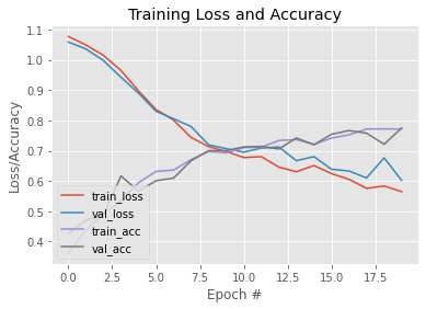
Name1 et al. / Electronic Letters on Computer Vision and Image Analysis 0(0):1-7, 2021 9
Figure 4: Data Augmentation
saddle points or the problem of local minima while training. We take the assistance of (Smith, 2017)’s approach
to find an optimal learning rate and set 1e-6 as the lower bound and 1e-3 as the upper bound for CLR. CLR
uses a step size of 8, and the model runs for 30 epochs with SGD the optimizer and categorical crossentropy as
the loss function
3.2.3 Fine tuning (ResNet50)
The upcoming models use transfer learning to improve the performance of the models. It is the process of
taking a network that is pre-trained on a dataset and using it to classify images on a different dataset. This
model implements transfer learning via fine-tuning on the ResNet50 architecture that is trained on ImageNet.
In the process of fine-tuning, the fully-connected nodes of the ResNet50, which make the predictions, are
removed. Instead, they are replaced by new fully-connected nodes with random initialization.
The earlier layers of the network are then frozen, and only the new fully-connected layers are trained. This
ensures that the previous robust features learned by the network are not lost, and the fully-connected layers are
trained to suit our specific classification task.
Once the network reaches a steady outcome, the entire network is then trained with a small learning rate.
This process allows the network to retain the already learned rich, discriminative filters and make necessary
changes to the newly connected fully-connected layers to learn patterns from the previous layers.
Our model includes a new set of 3 fully-connected layers followed by a dropout setting of rate 0.5. The
network, apart from the new set of layers, is frozen. Only the fully-connected layers are trained for 20 epochs
using SGD optimizer with a 1e-4 learning rate and 0.9 momentum along with categorical crossentropy as the
loss function. Data augmentation is performed too during the training. After this initial training, the network is
unfrozen, and the entire network is trained on again for 20 epochs with a 1e-5 learning rate.
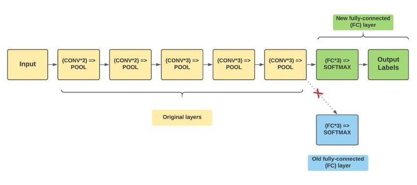
3.2.4 Fine tuning (VGG16)
This model follows the same fine-tuning process mentioned in the above model but with the VGG16 model pre-
trained on ImageNet. As can be seen from the figure [Figure 5], the old fully-connected layers are removed
from the VGG16 network and replaced by a new set of fully-connected layers. This new set of 3 fully-connected
layers is followed by a dropout setting of 0.5. The network, apart from the new set of layers, is frozen. Only
the fully-connected layers are trained for 20 epochs using SGD optimizer with a 1e-4 learning rate and 0.9
momentum along with categorical crossentropy as the loss function. Data augmentation is performed too
during the training. After this initial training, the network is unfrozen, and the entire network is trained on
again for 20 epochs with a 1e-5 learning rate.10 Name1 et al. / Electronic Letters on Computer Vision and Image Analysis 0(0):1-7, 2021 Figure 5: Old set of fully-connected layers in VGG16 network replaced by a new set of fully-connected layers 3.2.5 Feature Extraction (VGG16 This model implements transfer learning via feature extraction using the VGG16 network architecture pre- trained on the ImageNet. In this process, the pre-trained network is used as an arbitrary feature extractor. The VGG16 network is chopped off at a pre-specified layer. An image is allowed to propagate through this network, and the activations at the last layer are extracted. This is repeated for all the images in the dataset, and a feature vector is obtained for every image. The features are then trained on a standard machine learning model. As the feature extractor is a CNN, a non-linear model, they learn the non-linear features from the images. Moreover, because the feature vectors are very large with high dimensionality, training them on top of a linear model saves much time. In our model, we chop off the VGG16 network after the last maxpooling layer (before the fully-connected layers), as shown in [Figure 6]. The dimension of this last max-pooling layer is 7*7*512. Whenever an image is propagated through the network, the output is flattened to obtain a feature vector of 25,088- dim. We then use these feature vectors and train them using a logistic regression model. 4 Results and discussion There are five models which are trained on 2294 images and tested on 574 images. The baseline model follows a fundamental CNN architecture with no regularization methods. As is evident from the [Figure 9], it does not record good enough performance and achieves an accuracy of 77.53%. The second model, Baseline + Batch Normalization + Dropout, is an improvement over the baseline model. It integrates batch normalization, dropout, and data augmentation. Moreover, cyclical learning rate is used instead of a monotonically decreasing fixed learning rate. Moreover, an optimum learning rate is selected by using a learning rate finder method. To find the optimum learning rate, we select a very large upper bound (1e+1) and a very small lower bound (1e-10) on our learning rate. Then, we start training the network by starting from the lower bound and expo- nentially increasing the learning rate after every batch update. The training is continued until the upper bound on learning rate is reached. The loss after every batch update is recorded.
Name1 et al. / Electronic Letters on Computer Vision and Image Analysis 0(0):1-7, 2021         11

 Figure 6: Removing the fully-connected layers from VGG16 and treating the network as a feature extractor

   From figure [Figure 7], it is seen that when the learning rate is very low (less than 1e-6), the network is
unable to learn. Similarly, when the learning rate goes past 1e-3, the loss explodes because the learning rate
becomes too high for the model. Therefore, we choose 1e-6 for our lower bound and 1e-3 for the upper bound
for our cyclical learning rate [Figure 8].

                               Figure 7: Output of learning rate finder method
12 Name1 et al. / Electronic Letters on Computer Vision and Image Analysis 0(0):1-7, 2021
Figure 8: Cyclical behavior of the learning rate
Figure 9: Loss/Accuracy vs Epoch plot
(Baseline) Figure 10: Loss/Accuracy vs Epoch plot
(Baseline+Batch Normalization+Dropout)
The next model implements transfer learning via fine-tuning on the ResNet architecture. A new set of 3 fully
connected layers are added. During the initial training, the earlier network is frozen, and only the new layers
are trained. Out of a total of 26,342,787 parameters, only 2,755,075 parameters are trained. After this initial
training, the entire network is trained again. 26,275,779 parameters from a total of 26,342,787 are trained.
The model achieves an accuracy of 93.04%. The performance of the model is shown in [Figure 11]. The
same transfer learning process via fine-tuning is implemented in the next model but with the VGG network
architecture. The performance of the model is demonstrated in [Figure 12]. The model achieves an accuracy
of 93.57%.
It is evident from the above two models’ performance that transfer learning has drastically improved the
result compared to the earlier models. However, a sense of overfitting is acknowledged owing to the small size
of the dataset when using fine-tuning.
Our last model uses transfer learning via feature extraction on the VGG network architecture. The CNN is
used as a feature extractor, and the features are trained on a logistic regression model. This model outperforms
all the other previous models by recording an accuracy of 95%. Feature extraction serves as the optimum model
for our small-size dataset. The CNN captures the rich discriminative features from the images, and the machineName1 et al. / Electronic Letters on Computer Vision and Image Analysis 0(0):1-7, 2021 13
Figure 11: Loss/Accuracy vs Epoch plot Figure 12: Loss/Accuracy vs Epoch plot
(Fine tuning (ResNet50))) (Fine tuning (VGG16))
learning classifier helps us learn the underlying patterns of the features extracted from the CNN. The outputs
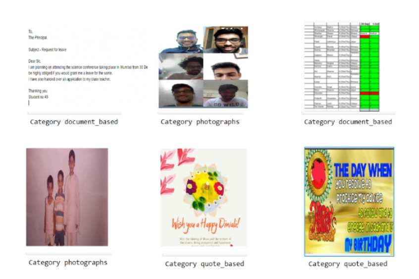
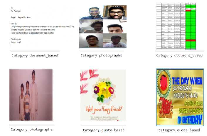
from a few test images are shown in [Figure 11], and all the models’ performance is compiled in [Table 2].
Figure 13: Result: CNN based efficient image classification system for smartphone device14 Name1 et al. / Electronic Letters on Computer Vision and Image Analysis 0(0):1-7, 2021
Model Accuracy
Baseline 77.53%
Baseline + Batch Normalization + Dropout 86.41%
Fine tuning (ResNet50) 93.04%
Fine tuning (VGG16) 93.57%
Feature extraction (VGG16) 95%
Table 2: Performance of all the models
5 Conclusion
Our research compared various models that used different deep learning techniques and architectures. Feature
extraction using the VGG16 network showed the best performance of all the models. We utilized the best deep
learning practices to successfully accomplish our goal to classify images present in smartphone devices. This
classifier opens up the opportunity to better manage and understand the plethora of images that make way into
our smartphone devices. Moreover, it paves the way to efficiently analyze the images that are shared across
social media platforms. Our approach also provides easy flexibility to accommodate other broad categories of
images that might emerge in the future or if a particular category is required to conquer a specific problem.
References
Ciregan, D., Meier, U., & Schmidhuber, J. (2012). Multi-column deep neural networks for image classification.
In 2012 ieee conference on computer vision and pattern recognition (pp. 3642–3649).
Gour, M., Jain, S., & Sunil Kumar, T. (2020). Residual learning based cnn for breast cancer histopathological
image classification. International Journal of Imaging Systems and Technology, 30(3), 621–635.
He, K., Zhang, X., Ren, S., & Sun, J. (2016, June). Deep residual learning for image recognition. In Proceed-
ings of the ieee conference on computer vision and pattern recognition (cvpr).
Ioffe, S., & Szegedy, C. (2015). Batch normalization: Accelerating deep network training by reducing internal
covariate shift.
Kölsch, A., Afzal, M. Z., Ebbecke, M., & Liwicki, M. (2017). Real-time document image classification
using deep cnn and extreme learning machines. In 2017 14th iapr international conference on document
analysis and recognition (icdar) (Vol. 1, pp. 1318–1323).
Krizhevsky, A., Sutskever, I., & Hinton, G. E. (2012). Imagenet classification with deep convolutional neural
networks. Advances in neural information processing systems, 25, 1097–1105.
LeCun, Y., Boser, B., Denker, J. S., Henderson, D., Howard, R. E., Hubbard, W., & Jackel, L. D. (1989).
Backpropagation applied to handwritten zip code recognition. Neural computation, 1(4), 541–551.
Levine, S., Pastor, P., Krizhevsky, A., Ibarz, J., & Quillen, D. (2018). Learning hand-eye coordination for
robotic grasping with deep learning and large-scale data collection. The International Journal of Robotics
Research, 37(4-5), 421–436.
Liu, S., & Deng, W. (2015). Very deep convolutional neural network based image classification using small
training sample size. In 2015 3rd iapr asian conference on pattern recognition (acpr) (pp. 730–734).
Simonyan, K., & Zisserman, A. (2015). Very deep convolutional networks for large-scale image recognition.
Smith, L. N. (2017). Cyclical learning rates for training neural networks. In 2017 ieee winter conference on
applications of computer vision (wacv) (pp. 464–472).
Song, L., Liu, J., Qian, B., Sun, M., Yang, K., Sun, M., & Abbas, S. (2018). A deep multi-modal cnn for multi-
instance multi-label image classification. IEEE Transactions on Image Processing, 27(12), 6025–6038.Name1 et al. / Electronic Letters on Computer Vision and Image Analysis 0(0):1-7, 2021 15
Srivastava, N., Hinton, G., Krizhevsky, A., Sutskever, I., & Salakhutdinov, R. (2014). Dropout: A simple way
to prevent neural networks from overfitting. Journal of Machine Learning Research, 15(56), 1929-1958.
Retrieved from http://jmlr.org/papers/v15/srivastava14a.html
Sun, Y., Xue, B., Zhang, M., Yen, G. G., & Lv, J. (2020). Automatically designing cnn architectures using the
genetic algorithm for image classification. IEEE transactions on cybernetics, 50(9), 3840–3854.
Szegedy, C., Liu, W., Jia, Y., Sermanet, P., Reed, S., Anguelov, D., . . . Rabinovich, A. (2015, June). Go-
ing deeper with convolutions. In Proceedings of the ieee conference on computer vision and pattern
recognition (cvpr).
Tianyu, Z., Zhenjiang, M., & Jianhu, Z. (2018). Combining cnn with hand-crafted features for image classifi-
cation. In 2018 14th ieee international conference on signal processing (icsp) (pp. 554–557).
Zeiler, M. D., & Fergus, R. (2013). Visualizing and understanding convolutional networks.
Zhao, Y., Hao, K., He, H., Tang, X., & Wei, B. (2020). A visual long-short-term memory based integrated cnn
model for fabric defect image classification. Neurocomputing, 380, 259–270.Figures Figure 1 The proposed system work ow Figure 2 Network architecture of baseline model
Figure 3

The difference between a standard neural network and a neural network after applying dropout

Figure 4

Data Augmentation
Figure 5

Old set of fully-connected layers in VGG16 network replaced by a new set of fully-connected layers

Figure 6

Removing the fully-connected layers from VGG16 and treating the network as a feature extractor
Figure 7

Output of learning rate nder method

Figure 8

Cyclical behavior of the learning rate
Figure 9

Loss/Accuracy vs Epoch plot (Baseline)

Figure 10

Loss/Accuracy vs Epoch plot (Baseline+Batch Normalization+Dropout)
Figure 11

Loss/Accuracy vs Epoch plot (Fine tuning (ResNet50)))

Figure 12

Loss/Accuracy vs Epoch plot (Fine tuning (VGG16))
Figure 13

Result: CNN based e cient image classi cation system for smartphone device
You can also read