PLS-SEM: THE HOLY GRAIL FOR ADVANCED ANALYSIS - Marketing Management ...
←
→
Page content transcription
If your browser does not render page correctly, please read the page content below
PLS-SEM: The Holy Grail for Advanced Analysis                                     Matthews, Hair and Matthews

       PLS-SEM: THE HOLY GRAIL FOR ADVANCED ANALYSIS
                               LUCY MATTHEWS, Middle Tennessee State University
                                  JOE HAIR, The University of South Alabama
                                  RYAN MATTHEWS, RLM Enterprises, LLC

    Advanced analytical techniques are reviewed for researchers wanting to expand their knowledge of
    how partial least squares structural equation modeling (PLS-SEM) facilitates better understanding
    of complex data relationships. We provide a brief overview of the differences between covariance-
    based structural equation modeling (CB-SEM) and PLS-SEM along with guidelines for the
    appropriate application of each. The focus is on mediation, moderation, multi-group analysis, and
    hierarchical component models. We also summarize several emerging analytical tools available with
    PLS-SEM. The ease of applying these advanced analytical techniques in many different research
    contexts makes PLS-SEM the “holy grail” for advanced analysis.

                        INTRODUCTION                         several of the more advanced analytical tools
                                                             available when applying PLS-SEM.
    For many researchers, keeping up with
    advanced methods can seem daunting. Learning             PLS-SEM versus CB-SEM
    new software along with the application and
    interpretation guidelines can sometimes be               When it comes to structural equations modeling
    overwhelming. That is not the case, however,             (SEM), researchers have a choice of two
    with partial least squares structural equation           methods: covariance-based SEM (CB-SEM;
    modeling (PLS-SEM), particularly using                   Jöreskog, 1978, 1993) and variance-based
    SmartPLS 3.0 (Ringle, Wende, & Becker,                   partial least squares (PLS-SEM; Lohmöller,
    2015). The recent rise in popularity of PLS-             1989; Wold, 1982). A fundamental distinction
    SEM can be attributed, at least in part, to the          between the two approaches is that CB-SEM is
    ease of understanding and applying the basic             based on the common factor model, while PLS-
    analytical tools of the method (Hair, Ringle, &          SEM is based on the composite factor model
    Sarstedt, 2011). But learning to apply advanced          (Hair, Hult, Ringle, & Sarstedt, 2017). With
    methods such as mediation, moderation, multi-            common factor models, the analysis is based
    group analysis and more, is also relatively              only on the common variance in the data.
    straightforward.                                         Therefore, the solution begins by calculating
                                                             the covariances between the variables in the
    Most researchers are at least somewhat familiar          study and only that common variance is used in
    with covariance-based structural modeling (CB-           the analysis (Hair, Matthews, Matthews, &
    SEM), most often run with the AMOS or                    Sarstedt, 2018; Sarstedt, Hair, Ringle, Theile, &
    LISREL software. Few researchers are aware               Gudergan, 2016). With the composite factor
    of and understand the fundamentals of variance           model the constructs and their scores are
    -based structural modeling (PLS-SEM). The                represented by the total variance in the
    purpose of this paper is to introduce and                indicators, not just common variance that is the
    provide an overview of the rapidly emerging              case with CB-SEM (Hair, Hult, Ringle, &
    method of variance-based structural equation             Sarstedt, 2017). In addition, the statistical
    modeling. In this paper, we first explain the            objectives are substantially different between
    differences in variance-based structural                 the two methods.          Using CB-SEM, the
    equation modeling (PLS-SEM) and the                      statistical objective is to estimate model
    covariance-based CB-SEM method, and                      parameters that minimize the differences
    therefore the rationale for the selection of one         between the observed sample covariance
    approach over another. We then summarize                 matrix, which is calculated before the
    The Marketing Management Journal                         theoretical model solution is obtained, with the
    Volume 28, Issue 1, Pages 1-13
    Copyright © 2018, The Marketing Management Association
                                                             covariance matrix that is estimated after the
    All rights of reproduction in any form reserved          theoretical model solution is obtained (Hair,
                                                             Sarstedt, Ringle, & Mena, 2012). If goodness of
1                                                                  Marketing Management Journal, Spring 2018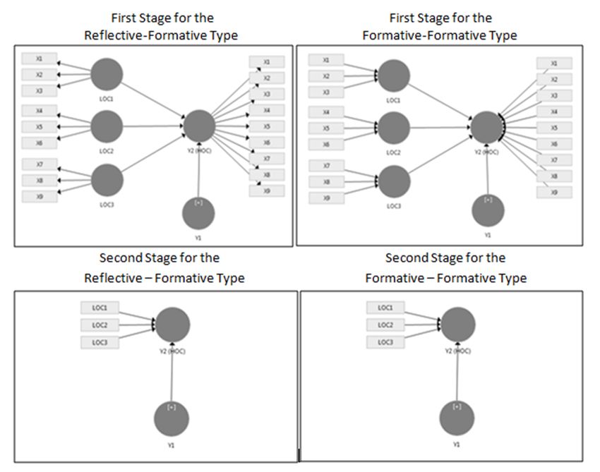
PLS-SEM: The Holy Grail for Advanced Analysis                              Matthews, Hair and Matthews

 fit is (GOF) demonstrated, the theoretical          order models, multi-group analysis, invariance
 structural model is confirmed. But if GOF is        and unobserved heterogeneity, making PLS-
 not possible the model is not confirmed. In         SEM a “go to” methodology for researchers.
 contrast, when using PLS-SEM, the statistical
 objective is to maximize the variance explained     Mediation
 in the dependent variable(s) (Hair, Sarstedt,
 Pieper, & Ringle, 2012a). Thus, the focus of        When a third variable, called a mediator,
 PLS is on optimizing prediction of the              intervenes between two other variables, the
 endogenous constructs and not on fit, which is      opportunity arises to examine mediation (Baron
 the focus of CB-SEM. Moreover, PLS-SEM is           & Kenny, 1986). Specifically, a change in the
 a variance-based approach and the analysis          exogenous construct produces a change in the
 does not start or end with a covariance matrix.     mediator variable, which then produces a
 Thus, a Chi-square type of GOF is not possible.     change in the endogenous construct, and the
                                                     mediator variable dictates the nature of the
 Determining when the application of each of         relationship between the exogenous and
 the methods is appropriate is straightforward. If   endogenous constructs (Hair, Hult, et al., 2017).
 the focus of the research is theory testing and     A crucial prerequisite for investigating
 confirmation (Sarstedt, Ringle, Henseler, &         mediating effects is strong apriori theoretical
 Hair, 2014), then CB-SEM is the appropriate         support (Preacher & Hayes, 2008).
 method. But if prediction, theory development
 and explanation are the focus of the research,      The foundation for mediation is a well-
 then PLS-SEM is the more appropriate method.        established theoretical relationship (c) between
 PLS-SEM is somewhat similar, both                   an exogenous (Y1) construct and an endogenous
 conceptually and practically, to using multiple     (Y3) construct (Figure 1) (Preacher & Hayes,
 regression analysis (Hair et al., 2011). But        2008). Testing for mediation in a model
 unlike multiple regression, PLS-SEM can be          requires a series of analyses beginning with
 applied to better understanding more complex        testing the significance of the indirect effect (a
 structural measurement and path models. At the      b) via the mediator variable (Y2) as seen in
 same time, PLS-SEM and CB-SEM are both              Figure 2. If the indirect effect is not significant,
 appropriate for metric data and reflective          then Y2 is not operating as a mediator in the
 measurement models. But PLS-SEM can easily          relationship. However, if (a b) is significant,
 be used with formative measurement models,          then the next test is to check the direct effect in
 non-metric data (e.g., ordinal & nominal),          the mediated model (c’). If c’ is not significant,
 continuous moderators, higher order models,         indirect-only (full) mediation has occurred.
 when latent variable scores are needed for          This occurs when the indirect effect is
 further analysis, and with small sample sizes (N    significant, but not the direct effect in the
 ≤ 100) as well as large samples (Hair,              mediated model.         Alternatively, if c’ is
 Hollingsworth, Randolph, & Chong, 2017).            significant, then partial mediation has occurred.
 Because it is nonparametric, PLS-SEM also has       When (a b c’) is positive, then complementary
 a wider application and greater flexibility in      mediation has occurred, but if (a b c’) is
 handling various modeling situations where it is    negative then competitive mediation has
 difficult to meet rigorous assumptions, such as     occurred (Hair, Hult, et al., 2017).
 a normal distribution and homoscedasticity, that
 are typically required with more traditional
                                                                     FIGURE 1:
 multivariate statistics (Vinzi, Chin, Henseler, &            Direct Effect of Exogenous
 Wang, 2010).          Therefore, PLS-SEM is               Variable on Endogenous Variable
 appropriate for exploratory research, theory
 development, and prediction.          It can be
                                                                           c
 executed on both small and large samples sizes,
 with reflective or formative measurement
 models, and does not assume the data has a               Y1                                 Y3
 normal distribution. Finally, the method can be
 used with metric and non-metric data,
 continuous moderators, secondary data, higher

Marketing Management Journal, Spring 2018                                                                   2
PLS-SEM: The Holy Grail for Advanced Analysis Matthews, Hair and Matthews
FIGURE 2: complementary and competitive mediation
Indirect Effect - Mediation Model (Hair, Hult, et al., 2017). With complementary
mediation, the mediated effect (a b) and direct
effect (c’) both exist and point in the same
direction (i.e., the signs are either both positive
Y2
or both negative), while with competitive
a b mediation, the mediated effect (a b) and direct
effect (c’) are both present and point in opposite
directions (i.e., a sign for one relationship is
positive and the other relationship is negative)
c’ (Zhao, Lynch, & Chen, 2010).
Y1 Y3
The most common types of mediation are
simple mediation analysis and multiple
mediation analysis. Simple mediation analysis
is when one mediator variable is specified in
Mediation has traditionally been executed using the structural model. Often times, however,
multiple regression. Baron and Kenny (1986) exogenous constructs influence endogenous
and more recently the PROCESS approach by constructs through more than one mediating
Preacher and Hayes (2008) both focus on variable requiring multiple mediation analyses
multiple regression and examine significance in (Hair, Hult, et al., 2017). The mediators reveal
mediation using the Sobel test, which assumes the “real” relationship among the exogenous
the data are normally distributed. The and endogenous constructs. Figure 3 depicts a
advantages of using PLS-SEM for mediation model with two mediating variables, Y2 and Y4.
are that bootstrapping makes no assumptions The direct effect is measured by c’. But the
about the shape of the variables’ distribution or indirect effect of Y1 on Y3 now includes the Y4
the sampling distribution of the statistics, and mediator (d e) in addition to Y2, and the total
all the mediated relationships are tested indirect effect of Y1 on Y3 is measured by the
simultaneously instead of separately, which sum of the two indirect effects (i.e., a b + d e).
reduces bias (Hair, Sarstedt, Hopkins, & Therefore, the total effect of Y1 on Y3 is the
Kuppelwieser, 2014). Finally, mediation sum of the direct effect and the total indirect
testing using PLS-SEM can be applied with effect (i.e., c’ + a b + d e).
smaller sample sizes while yielding higher
levels of statistical power compared to prior Analyzing all mediators concurrently allows for
testing methods like the parametric Sobel a more thorough understanding of the overall
(1982) test. effect. If each mediator were analyzed in a
simple mediation analysis (i.e., with a
Path models that include a mediator are still regression model where all relationships are
required to meet the quality criteria of the tested separately), the indirect effect would
measurement models. For formative likely be overstated due to the correlation of
measurement models, convergent validity one mediator to another (Hair, Hult, et al.,
(redundancy), collinearity between indicators, 2017). When PLS-SEM is used, multiple
and significance/relevance of outer weights are mediation in which all relationships (direct and
required (Hair, Hult, et al., 2017). For indirect) are tested simultaneously is possible.
reflective measurement models, the quality Thus, with multiple mediation the impact of
criteria include internal consistency reliability, one or multiple mediators can be tested
convergent validity, and discriminant validity. simultaneously, eliminating the overstatement
It is important to also confirm that collinearity of the correlation associated with each
in the structural model is not at a critical level mediator.
since biased path coefficients may incur. When
high collinearity exists, the direct effect may The steps for processing multiple mediation
suggest nonmediation via nonsignificance or an analyses are the same as in simple mediation
unexpected sign change may result in an analysis. The testing process begins with
erroneous differentiation between examining the significance of each indirect
3 Marketing Management Journal, Spring 2018PLS-SEM: The Holy Grail for Advanced Analysis Matthews, Hair and Matthews
effect, and then the direct effect between the When including a moderator in the model, the
exogenous and endogenous constructs. To variable will appear twice, once as the variable
determine the total indirect effect manual itself (main effect) and again as the interaction
calculations of the standard error for each effect (a combination of the main effect and the
specific indirect effect may be necessary. moderator; see Figure 4). Unlike mediation
Using SmartPLS 3.0 (Ringle et al., 2015), where the exogenous construct acts as an
however, this can be accomplished by simply antecedent to the mediator, in moderation the
obtaining the indirect effects results of the moderator variable and exogenous construct
bootstrapping routine and using spreadsheet interact (Y1*M) at the same level to impact the
software such as Microsoft Excel. Finally, to endogenous variable. This is a multiplicative
calculate the t value of the specific indirect relationship.
effect, divide the specific indirect effect by the
standard error (Hair, Hult, et al., 2017). FIGURE 4:
Moderation Model
FIGURE 3:
Multiple Mediation Model
Y1 M
Y2
M
c
a b b
a
c’
Y1 Y2
Y1 Y3
d e While several analytical procedures exist for
estimating the measurement model with
moderation (e.g., product indicator approach,
orthogonalizing approach, and two-stage
Y4 approach), the two-stage approach is typically
recommended. The two-stage approach is able
to handle both reflective and formative
Moderation moderators and additional exogenous constructs
in the path model. Moreover, compared to the
Moderation (interaction effect) occurs when the other approaches, the two-stage approach
relationship between two constructs varies exhibits higher levels of statistical power (Hair,
depending on a third (moderator) variable Hult, et al., 2017).
(Henseler & Chin, 2010). The variation can
influence the strength or direction of the The two-stage approach begins by running the
relationship (Baron & Kenny, 1986). main effects model without the moderation
Moderator variables can be categorical (e.g., interaction term in the model to estimate the
age, income, gender) and tested by means of latent variable scores (Henseler & Chin, 2010).
group comparisons using either PLS-SEM or In the second stage, the latent variable scores
CB-SEM. Alternatively, with PLS-SEM from stage one of the exogenous latent variable
moderators can also be a continuous variable and the moderator variables are multiplied to
(e.g., attitudes about satisfaction, loyalty, create a single-item measure to represent the
commitment, brand passion) typically measured interaction term (Hair, Hult, et al., 2017). At the
using multi-item scales (note that continuous same time, all the other latent variables are
moderators cannot be used with CB-SEM). represented by a single item measure (latent
Marketing Management Journal, Spring 2018 4PLS-SEM: The Holy Grail for Advanced Analysis Matthews, Hair and Matthews
variable score) that was calculated in stage one. f2 effect size is examined. The f2 measures the
The moderator hypothesis is supported if the extent to which the endogenous latent variable
interaction effect (c) is significant (Hair, is explained by the moderation. The f2 effect
Sarstedt, Ringle, & Gudergan, 2018). sizes of 0.02, 0.15, and 0.35 suggest small,
medium, and large effect sizes, respectively
The results indicate that the value of c (Cohen, 1988).
(interaction effect) represents the strength of the
relationship between Y1 and Y2 when the Interpreting and drawing conclusions from the
moderator variable M has a value of zero (Hair, moderation results can be difficult. Slope plots
Hult, et al., 2017). However, since many scales are typically used as a visual illustration to gain
either do not include a value of zero or a value a better understanding of the moderation effect.
of zero does not make sense, standardization is Figure 5 displays a two-way interaction of the
often necessary. Standardization facilitates relationship between Y1 and Y2. The horizontal
interpretation as well as reduces collinearity x-axis represents the exogenous construct (Y1)
among the exogenous construct, the moderator, and the vertical y-axis represents the
and the interaction term. To standardize, the endogenous construct (Y2). The two lines
variable’s mean is subtracted from each illustrate the relationship between Y1 and Y2 for
observation and divided by the variable’s both low and high levels of the moderator
standard error (Sarstedt & Mooi, 2014). When construct (M). The low level of M (solid line)
using SmartPLS 3, the software executes many is one standard deviation unit below the
types moderation, standardizes when necessary, average, while the high level of M (dotted line)
and produces a simple slope analysis for is one standard deviation unit above the
interpreting moderation results. average. There is a negative moderating effect
of -0.80 between the interaction term and the
To assess the impact on the R2 value when the endogenous construct. The high moderator’s
interaction effect is omitted from the model, the slope is relatively flat but decreases slightly as
FIGURE 5:
Graphical Illustration of Moderation Effect
5 Marketing Management Journal, Spring 2018PLS-SEM: The Holy Grail for Advanced Analysis Matthews, Hair and Matthews
the exogenous variable changes from low to enough (See Hair, Hult, et al., 2014).
high. Thus, the relationship between Y1 and Y2 Additionally, the subgroups should be similar
becomes weaker with high levels of the in size to avoid introducing error (Becker, Rai,
moderator construct. But for low levels of the Ringle, & Volckner, 2013).This involves
moderator variable, the slope is quite steep and coding the master data file into subgroups that
the relationship between Y1 and Y2 becomes can be executed with PLS-SEM (Matthews,
much stronger with high levels of M. To 2017).
facilitate interpretation of the interaction,
SmartPLS 3 computes and the output displays a While a number of approaches can be used to
simple slope plot. compare the path coefficients of the group
SEMs, most researchers recommend the
Multi-Group permutation test (Hair, Sarstedt, Ringle, &
Gudergan, 2018). Permutation is non-
Multi-group analysis (MGA) or between-group parametric and more conservative than the
analysis is a means of testing apriori defined parametric test, and controls well for Type 1
groups to determine if there are significant error (Henseler, Ringle, & Sarstedt, 2016). To
differences in group-specific parameter execute the permutation test, the correlations
estimates (e.g., outer weights, outer loadings between the composite scores using the weights
and path coefficients) obtained when using PLS obtained from the first group are computed
-SEM (Hair, Hult, Ringle, & Sarstedt, 2014; against the composite scores using the weights
Henseler & Chin, 2010). By applying MGA, obtained from the second group during each
researchers are able to test for differences permutation run (Henseler et al., 2016).
between two identical models for different
apriori specified groups within the data set. In The focus of multi-group analysis is to examine
contrast to standard approaches to testing the path coefficients of the theoretical models
moderation, which examine a single structural for the two groups to determine if they are
relationship at a time, MGA via PLS-SEM is an significantly different. This begins by running
efficient way to assess moderation across the model for each group separately, using the
multiple relationships (Hair, Sarstedt, Ringle, et guidelines set out for evaluation of a
al., 2012). measurement model (Hair, Hult, et al., 2014,
2017). This determines if there are group
This type of analysis enables researchers to specific differences. Then, it is necessary to
identify differences between the structural paths determine if the difference between the two
of multiple groups. For example, Matthews groups is significant, which can be
(2017) illustrated how skill discrepancy accomplished by running the Permutation Test.
partially mediates the relationship between A permutation p-value of less than or equal to
autonomy and cognitive engagement for male 0.10 indicates a significant difference between
salespeople, but not for female salespeople. the two groups being compared (Matthews,
PLS-MGA also facilitates a more accurate and 2017).
comprehensive assessment of group differences
and strategy implementation based on more MGA allows researchers to determine
specific outcomes for the heterogeneous groups significant differences among observed
in the data (Matthews, 2017). Finally, the characteristics. These differences may not be
differences identified can be used to highlight evident in aggregate data since significant
the potential error if these subpopulations are positive and negative group-specific results
considered a single homogeneous group may offset one another resulting in non-
(Schlagel & Sarstedt, 2016). significant relationships (Hair, Hult, et al.,
2017). Although the path coefficients for the
The first step in conducting MGA involves subdivided groups will often display numerical
generating data groups that are based on the differences, MGA assists in identifying when
categorical variable of interest (e.g., gender, those differences are statistically significant.
country of origin, age, or income). Once the
data is subdivided, it is necessary to ensure that
the sample sizes of the new subgroups are large
Marketing Management Journal, Spring 2018 6PLS-SEM: The Holy Grail for Advanced Analysis Matthews, Hair and Matthews
Hierarchical Component Models structural model, making the model more
parsimonious and easier to understand. In
Hierarchical component models (HCM), or addition, introducing a HCM into a structural
higher order models, involve testing model can reduce multicollinearity among first-
measurement structures that contain two layers order constructs, or formative indicators that
of constructs, the higher order component exhibit high levels of collinearity. In either
(HOC) of the model and the lower order situation, the use of HCMs should be supported
component (LOC). An example of a HCM is by theory. Note that higher order models can
when lower order components of job also be used with CB-SEM, but the
satisfaction are specified as multi-faceted and assumptions are much more restrictive and
the higher order component is a single overall therefore limit their application with that
construct of job satisfaction. Figure 6 displays a method.
theoretical HCM for job satisfaction that
includes the LOCs (lower order components) There are four main types of HCMs (Jarvis,
and the HOC (higher order component). In the MacKenzie, & Podsakoff, 2003; Wetzels,
figure, the LOCs represent the first-order multi- Odekerken-Schroder, & van Oppen, 2009) used
item constructs for job satisfaction, and the in PLS-SEM models (Ringle, Sarstedt, &
HOC is the second-order overall (combined) Straub, 2012). The HCM model begins with the
construct for job satisfaction. Researchers may lower-order components (LOCs), which are
find the use of a HCM helpful when trying to used to make up the higher-order component
reduce the number of relationships in the (HOC) (Hair, Hult, et al., 2017). Each model is
FIGURE 6:
Hierarchical Component Model for Multi-faceted Job Satisfaction
7 Marketing Management Journal, Spring 2018PLS-SEM: The Holy Grail for Advanced Analysis Matthews, Hair and Matthews
characterized by the different relationships the underlying components LOC1, LOC2, and
between the LOCs and the HOC as well as the LOC3 in the measurement model. However,
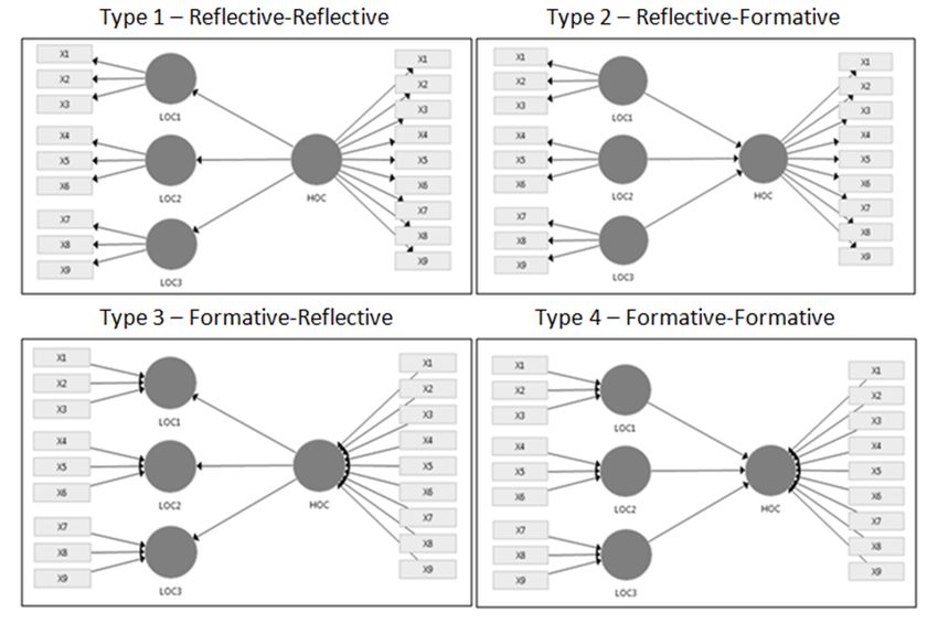
indicators with each construct. The first type is some issues arise using the repeated indicator
the Reflective-Reflective, where the indicator approach when the model is formative-
measures for the first order components are formative (type 4) or reflective-formative
reflective and the measures from the LOC to (type 2). In this situation, when the relationship
the HOC are reflective (Figure 7). Type two is from the LOC to the HOC is formative, almost
Reflective-Formative. For this model, the LOC all of the HOC variance is explained by the
indicators are reflective but the LOC to the LOC (R2 close to 1.0). This can be an issue if
HOC is formative. Type three is Formative- there are other relationships pointing to the
Reflective, such that the first-order indicators HOC, as they will have a very small and
are measured formatively and the HOC from insignificant impact. Therefore, for type 2 and
the LOC is reflective. The final type (type type 4 models, a two-stage HCM analysis
four), is Formative-Formative where the should be used (Hair, Hult, et al., 2017).
indicators of the first-order are measured Similar to the two-stage approach for
formatively and the measures from the LOC to moderation, in stage one the repeated indicator
the HOC are formative. approach is used to obtain the latent variable
scores for the LOCs. Then in the second stage,
When creating the HOC in PLS-SEM, all the the LOC constructs and first-order indicators
indicators from the LOC are assigned to the used for the HOC are replaced with latent
HOC using a repeated indicators approach variable scores for the LOC from stage one
(Hair, Hult, et al., 2017). Therefore, the (Figure 8). The two-stage HCM analysis
indicators for the HOC x 1 to x 9 are the same as
FIGURE 7:
Four Types of Hierarchical Component Models
Marketing Management Journal, Spring 2018 8PLS-SEM: The Holy Grail for Advanced Analysis Matthews, Hair and Matthews
allows other latent variables outside of the understanding and explaining the outcomes of
HOC to explain some of the variance. this technique (e.g., Becker, Klein, & Wetzels,
2012; Kuppelwieser & Sarstedt, 2014; Ringle et
When using HCM it is important that a similar al., 2012).
number of indicators are used for all the LOCs.
Otherwise, the relationship between the HOC Other Advanced Topics
and the LOC can be biased due to the
disproportionate number of indicators (Hair, In addition to the topics addressed above,
Hult, et al., 2017). Note that the number of researchers have further opportunities to
indicators on the LOCs does not have to be improve their analysis and understanding of
equal (as shown in Figures 6 & 7), but should theoretical relationships. Measurement model
be comparable. Additionally, for the inner PLS invariance, which tests datasets for differences
path model, not all algorithmic weighting in measurement model estimates, is a useful
schemes apply when estimating HCMs in PLS- tool that should be combined with multigroup
SEM. In particular, the centroid weighting analysis. By employing the measurement
scheme should not be used (Hair, Sarstedt, invariance of composite models (MICOM)
Ringle, et al., 2012). Prior research using and procedure (Henseler et al., 2016), configural
explaining HCM models can further assist in and compositional invariance can be
FIGURE 8:
Two-Stage Approach for HCM Analysis
9 Marketing Management Journal, Spring 2018PLS-SEM: The Holy Grail for Advanced Analysis Matthews, Hair and Matthews
established. Doing so ensures that variations in Summary
the path relationships between latent variables
is a result of the true differences in the When analyzing research that requires
structural relationships, and is not the result of advanced analytical approaches, it is important
different meanings in the groups’ responses to understand the differences between CB-SEM
attributed to the phenomena being measured and PLS-SEM, as well as other multivariate
(Hair, Hult, et al., 2017; Henseler et al., 2016). analysis methods. Because PLS-SEM has a
Failure to establish data equivalence using much greater capacity for handling a variety of
MICOM may potentially result in measurement modeling issues and does not impose restrictive
error and thus misleading results (Hult et al., assumptions (Vinzi et al., 2010), the use of PLS
2008), reduce the overall power of the -SEM is highlighted. For mediation, the
statistical tests, and influence the precision of advantage of using PLS-SEM is the lack of
the estimators (Hair, Hult, et al., 2017). restrictive distribution assumptions, the
flexibility to execute with both formative and
The importance-performance map analysis reflective measurement models, and the ability
(IPMA), or importance-performance matrix to yield higher levels of statistical power with
analysis, displays the structural model total smaller sample sizes, while overcoming the
effects on a specific endogenous construct. The limitations of multiple regression approaches
total effects of the predecessor variables are (Hair, Sarstedt, et al., 2014). The two-stage
used to assess each exogenous construct’s approach for moderation using PLS-SEM
importance in shaping the endogenous exhibits high levels of statistical power and is
construct. The average latent variable scores of capable of handling both reflective and
the exogenous constructs measure their formative moderators when the structural
performance (Hair, Hult, et al., 2017) using a model includes other exogenous constructs.
rescaling technique (Höck, Ringle, & Sarstedt, Multi-group analysis via permutation in PLS-
2010). Combined, researchers can identify SEM enables researchers to easily identify
constructs with relatively high importance heterogeneous groups in the data to more
(strong total effect) and low performance (low accurately assess group differences (Matthews,
average latent variable scores) as areas for 2017). Finally, higher order component models
further research. IPMA can be conducted at the (HCMs) can be applied with PLS-SEM to
indicator level as well to identify and improve obtain more accurate solutions for structural
upon those indicators that are most relevant. models exhibiting high multicollinearity.
Finally, rather than using a priori characteristics Beyond these advanced analysis approaches,
to partition datasets into groups, as was PLS-SEM can: (1) establish data equivalence
described in multi-group analysis, tools like via the three stage MICOM process (Henseler
finite mixture PLS (FIMIX-PLS, Sarstedt, et al., 2016) to minimize measurement error, (2)
Becker, Ringle, & Schwaiger, 2011) or identify the importance and performance of
prediction-oriented segmentation (FIMIX-POS, antecedent constructs to target areas for further
Sarstedt, Ringle, & Hair, 2017) can be used to research (Hair, Hult, et al., 2017), and (3)
uncover unobserved heterogeneity. Since uncover unobserved heterogeneity so structural
sources of heterogeneity in the data aren’t and measurement models can be examined
always known a priori, identifying and treating either at the individual group level or the
unobserved heterogeneity allows researchers to aggregate level (Matthews et al., 2016; Hair et
feel confident about analyzing data at an al. 2016). Therefore, when facing complex
aggregate level (Hair, Sarstedt, Matthews, & research models, even though there are a
Ringle, 2016). Examples of FIMIX-PLS are variety of multivariate methods available, the
available to aid researchers in the application to numerous flexible analysis options, limited
their own dataset (Matthews, Sarstedt, Hair, & assumptions, and user-friendliness of PLS-SEM
Ringle, 2016; Sarstedt, Schwaiger, & Ringle, make it the “holy grail” for advanced methods.
2009). Failure to consider heterogeneity may
also result in invalid outcomes (Becker et al.,
2013).
Marketing Management Journal, Spring 2018 10PLS-SEM: The Holy Grail for Advanced Analysis Matthews, Hair and Matthews
REFERENCES Hair, J. F., Sarstedt, M., Matthews, L. M., &
Ringle, C. M. (2016). Identifying and
Baron, R. M., & Kenny, D. A. (1986). The Treating Unobserved Heterogeneity with
moderator-mediator variable distinction in FIMIX-PLS: Part I - Method. European
social psychological research: Conceptual, Business Review, 28(1) 63-76.
strategic, and statistical considerations. Hair, J. F., Sarstedt, M., Pieper, T. M., &
Journal of Personality and Social Ringle, C. M. (2012). The Use of Partial
Psychology, 51(6), 1173-1182. Least Squares Structural Equation Modeling
Becker, J.-M., Klein, K., & Wetzels, M. (2012). in Strategic Management Research: A
Formative Hierarchical Latent Variable Review of Past Practices and
Models in PLS-SEM: Recommendations and Recommendations for Future Applications.
Guidelines. Long Range Planning, 45(5-6), Long Range Planning, 45(5-6), 320-340.
359-394. Hair, J. F., Sarstedt, M., Ringle, C. M., &
Becker, J.-M., Rai, A., Ringle, C. M., & Gudergan, S. P. (2018). Advanced Issues in
Volckner, F. (2013). Discovering unobserved Partial Least Squares Structural Equations
heterogeneity in structural equation models to Modeling (PLS-SEM). Thousand Oaks, CA,
avert validity threats. MIS Quarterly, 37(3), Sage.
665-694. Hair, J. F., Sarstedt, M., Ringle, C. M., &
Cohen, J. (1988). Statistical Power A nalysis for Mena, J. A. (2012). An Assessment of the use
the Behavioral Sciences. Mahwah, NJ: of Partial Least Squares Structural Equation
Lawrence Erlbaum. Modeling in Marketing Research. Journal of
Hair, J. F., Hollingsworth, C. L., Randolph, A. the Academy of Marketing Science, 40(3),
B., & Chong, A. (2017). An Updated and 414-433.
Expanded Assessment of PLS-SEM in Henseler, J., & Chin, W. W. (2010). A
Information Systems Research. Industrial Comparison of Approaches for the Analysis
Management & Data Systems (3), 442-458. of Interaction Effects Between Latent
Hair, J. F., Hult, G. T. M., Ringle, C. M., & Variables Using Partial Least Squares Path
Sarstedt, M. (2014). A Primer on Partial Modeling. Structural Equation Modeling: A
Least Squares Structural Equation Modeling Multidisciplinary Journal, 17(1), 82-109.
(PLS-SEM). Los Angeles, London, New Henseler, J., Ringle, C. M., & Sarstedt, M.
Delhi, Singapore, Washington DC: SAGE. (2016). Testing Measurement Invariance of
Hair, J. F., Hult, G. T. M., Ringle, C. M., & Composites Using Partial Least Squares.
Sarstedt, M. (2017). A Primer on Partial International Marketing Review, 33(3),
Least Squares Structural Equation Modeling 405-431.
(PLS-SEM) (2nd ed.). Los Angeles, London, Höck, C., Ringle, C. M., & Sarstedt, M. (2010).
New Delhi, Singapore, Washington DC: Management of Multi-purpose Stadiums:
SAGE. Importance and Performance Measurement of
Hair, J. F., Matthews, L. M., Matthews, R. L., Service Interfaces. International Journal of
& Sarstedt, M. (2017). PLS-SEM or CB- Services Technology and Management, 14(2-
SEM: Updated Guidelines on Which Method 3), 188-207.
to Use. International Journal of Multivariate Hult, G. T. M., Ketchen Jr, D. J., Griffith, D.
Data Analysis,1(2), 107-123. A., Finnegan, C. A., Gonzalez-Padron, T.,
Hair, J. F., Ringle, C. M., & Sarstedt, M. Harmancioglu, N., & et al. (2008). Data
(2011). PLS-SEM: Indeed a Silver Bullet. Equivalence in Cross-Cultural International
The Journal of Marketing Theory and Business Research: Assessment and
Practice, 19(2), 139-152. Guidelines. Journal of International Business
Hair, J. F., Sarstedt, M., Hopkins, L., & Studies, 39(6), 1027-1044.
Kuppelwieser, V. G. (2014). Partial least Jarvis, C. B., MacKenzie, S. B., & Podsakoff,
squares structural equation modeling (PLS- P. M. (2003). A Critical Review of Construct
SEM): An emerging tool in business Indicators and Measurement Model
research. European Business Review, 26(2), Misspecification in Marketing and Consumer
106-121. Research. Journal of Consumer Research, 30
(2), 199-218.
11 Marketing Management Journal, Spring 2018PLS-SEM: The Holy Grail for Advanced Analysis Matthews, Hair and Matthews
Jöreskog, K. G. (1978). Structural Analysis of Sarstedt, M., Ringle, C. M., & Hair, J. F. (2017).
Covariance and Correlation Matrices. Treating Unobserved Heterogeneity in PLS-
Psychometrika, 43(4), 443-477. SEM: A Multi-method Approach. In H. Latan
Jöreskog, K. G. (1993). Testing Structural & R. Noonan (Eds.), Partial Least Squares
Equation Models. In K. A. Bollen & J. S. Structural Equation Modeling - Basic
Long (Eds.), Testing Structural Equation Concepts, Methodological Issues and
Models (pp. 294-316). Newbury Park: Sage. Applications. Berlin: Springer International
Kuppelwieser, V., & Sarstedt, M. (2014). Publishing AG, 197-213.
Applying the Future Time Perspective Scale Sarstedt, M., Ringle, C. M., Henseler, J., & Hair,
to Advertising Research. International J. F. (2014). On the Emancipation of PLS-
Journal of Advertising, 33(1), 113-136. SEM: A Commentary on Rigdon (2012). Long
Lohmöller, J.-B. (1989). Latent V ariable Path Range Planning, 47(3), 154-160.
Modeling with Partial Least Squares. Sarstedt, M., Schwaiger, M., & Ringle, C. M.
Heidelberg: Physica. (2009). Do We Fully Understand the Critical
Matthews, L. M. (2017). Applying Multi-group Success Factors of Customer Satisfaction with
Analysis in PLS-SEM: A Step-by-Step Industrial Goods? Extending Festge and
Process. In H. Latan & R. Noonan (Eds.), Schwaiger's Model to Account for
Partial Least Squares Structural Equation Unobserved Heterogeneity. Journal of
Modeling - Basic Concepts, Methodological Business Market Management, 3(3), 185-206.
Issues and Applications. Berlin: Springer Schlagel, C., & Sarstedt, M. (2016). Assessing
International Publishing AG. the Measurement Invariance of the Four-
Matthews, L. M., Sarstedt, M., Hair, J. F., & Dimensional Cultural Intelligence Scale
Ringle, C. M. (2016). Identifying and Across Countries: A Composite Model
Treating Unobserved Heterogeneity with Approach. European Management Journal, 34
FIMIX-PLS: Part II - A Case Study. (6), 633-649.
European Business Review, 28(2) 208-224. Sobel, M. E. (1982). Asymptotic Confidence
Preacher, K. J., & Hayes, A. F. (2008). Intervals for Indirect Effects in Structural
Asymptotic and Resampling Strategies for Equations Models. Sociological Methodology,
Assessing and Comparing Indirect Effects in 13, 290-312.
Multiple Mediator Models. Behavior Vinzi, V. E., Chin, W. W., Henseler, J., &
Research Methods, 40(3), 879-891. Wang, H. (2010). Editorial: Perspectives on
Ringle, C. M., Sarstedt, M., & Straub, D. W. Partial Least Squares. In V. E. Vinzi, W. W.
(2012). A Critical Look at the use of PLS- Chin, J. Henseler, & H. Wang (Eds.),
SEM in MIS Quarterly. MIS Quarterly, 36 Handbook of Partial Least Squares: Concepts,
(1), iii-xiv. Methods and Applications. Heidelberg
Ringle, C. M., Wende, S., & Becker, J.-M. Dordrecht London New York: Springer.
(2015). Smartpls 3. Bonningstedt: SmartPLS. Wetzels, M., Odekerken-Schroder, G., & van
Retrieved from http://smartpls.com. Oppen, C. (2009). Using PLS Path Modeling
Sarstedt, M., Becker, J.-M., Ringle, C. M., & for Assessing Hierarchical Construct Models:
Schwaiger, M. (2011). Uncovering and Guidelines and Empirical Illustration. MIS
treating unobserved heterogeneity with Quarterly, 33, 177-195.
FIMIX-PLS: which model selection criterion Wold, H. (1982). Soft Modeling: The Basic
provides an appropriate number of segments? Design and Some Extentions. In K. G.
Schmalenbach Business Review, 63, 34-62. Jöreskog & H. Wold (Eds.), Systems Under
Sarstedt, M., Hair, J. F., Ringle, C. M., Theile, Indirect Observations: Part II (pp. 1-54).
K. O., & Gudergan, S. P. (2016). Estimation Amsterdam: North-Holland.
Issues with PLS and CBSEM: Where the
Bias Lies! Journal of Business Research, 69, GLOSSARY
3998-4010.
Sarstedt, M., & Mooi, E. A. (2014). A Concise Bootstrapping: a resampling technique that
Guide to Market Research: The Process, draws a specified (large) number of subsamples
Data, and Methods using IBM SPSS from the original data and using replacement,
Statistics (2nd ed.). Berlin: Springer. estimates models for each subsample. It is used
to assess statistical significance without relying
Marketing Management Journal, Spring 2018 12PLS-SEM: The Holy Grail for Advanced Analysis Matthews, Hair and Matthews on distributional assumptions to determine standard errors of coefficients. Collinearity: when two variables are highly correlated. Formative measurement model: a type of measurement model setup in which the direction of the arrows is from the indicator variables to the construct, thus indicating an assumption that the indicator variables cause the measurement of the construct. Orthogonalizing approach: an approach to model the interaction term when including a moderator variable in the model. This creates an interaction term with orthogonals indicators. In the moderator model, these orthogonal indictors are not correlated with independent variable indicators and the moderator variable indicators. Product indicator approach: an approach to model the interaction term when including a moderator variable in the model. This approach involves multiplying the indicators of the moderator with the indicators of the exogenous latent variable to establish a measurement model of the interaction term. The approach is only applicable when both moderator and exogenous latent variables are reflective. Reflective measurement: a type of measurement model setup in which measures the direction of the arrow is from the construct to the indicator variables, thus the measures represent the effects (or manifestations) of an underlying construct. Causality is from the construct to its measures (indicators). 13 Marketing Management Journal, Spring 2018
You can also read